
Water Dynamics in Fish Collagen Gels—Insight from NMR Relaxometry

 , , , , and
Abstract
:1. Introduction
2. Materials and Methods
2.1. Samples Preparation
2.2. NMR Relaxometry Experiments
2.3. Theory
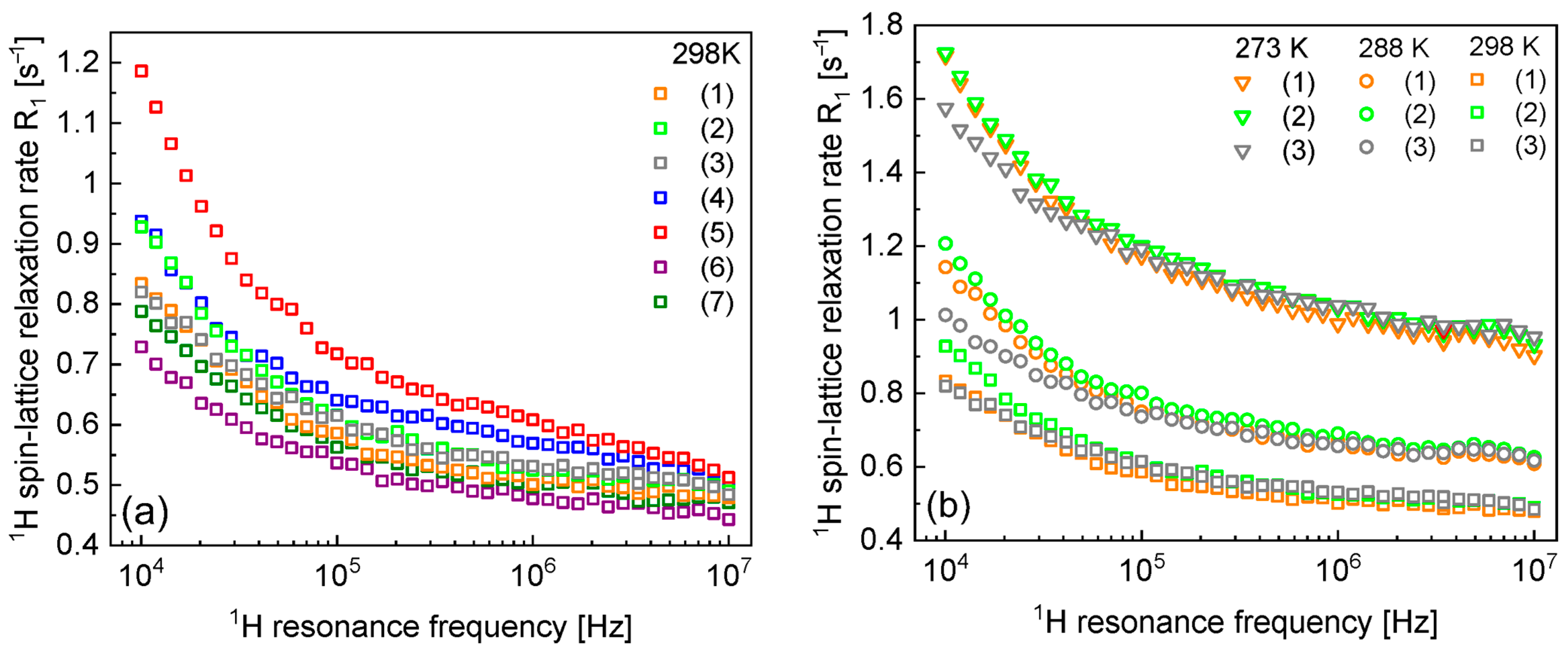
3. Results
4. Discussion
5. Conclusions
Author Contributions
Funding
Institutional Review Board Statement
Informed Consent Statement
Data Availability Statement
Conflicts of Interest
Appendix A


References
- Subhan, F.; Hussain, Z.; Tauseef, I.; Shehzad, A.; Wahid, F. A review on recent advances and applications of fish collagen. Crit. Rev. Food Sci. Nutr. 2020, 61, 1027–1037. [Google Scholar] [CrossRef] [PubMed]
- Furtado, M.; Chen, L.; Chen, Z.; Chen, A.; Cui, W. Development of fish collagen in tissue regeneration and drug delivery. Eng. Regen. 2022, 3, 217–231. [Google Scholar] [CrossRef]
- Wang, H. A Review of the Effects of Collagen Treatment in Clinical Studies. Polymers 2021, 13, 3868. [Google Scholar] [CrossRef] [PubMed]
- Salvatore, L.; Gallo, N.; Natali, M.L.; Campa, L.; Lunetti, P.; Madaghiele, M.; Blasi, F.S.; Corallo, A.; Capobianco, L.; Sannino, A. Marine collagen and its derivatives: Versatile and sustainable bio-resources for healthcare. Mater. Sci. Eng. C 2020, 113, 110963. [Google Scholar] [CrossRef]
- Liu, C. Application of marine collagen for stem-cell-based therapy and tissue regeneration. Med. Int. 2021, 1, 6. [Google Scholar] [CrossRef]
- Seyedlar, A.O.; Stapf, S.; Mattea, C. Nuclear magnetic relaxation and diffusion study of the ionic liquids 1-ethyl- and 1-butyl-3-methylimidazolium bis(trifluoromethylsulfonyl)imide confined in porous glass. Magn. Reson. Chem. 2019, 57, 818–828. [Google Scholar] [CrossRef]
- Seyedlar, A.O.; Stapf, S.; Mattea, C. Dynamics of the ionic liquid 1-butyl-3-methylimidazolium bis(trifluoromethylsulphonyl)imide studied by nuclear magnetic resonance dispersion and diffusion. Phys. Chem. Chem. Phys. 2014, 17, 1653–1659. [Google Scholar] [CrossRef]
- Wencka, M.; Apih, T.; Korošec, R.C.; Jenczyk, J.; Jarek, M.; Szutkowski, K.; Jurga, S.; Dolinšek, J. Molecular dynamics of 1-ethyl-3- methylimidazolium triflate ionic liquid studied by 1H and 19F nuclear magnetic resonances. Phys. Chem. Chem. Phys. 2017, 19, 15368–15376. [Google Scholar] [CrossRef]
- Kruk, D.; Masiewicz, E.; Wojciechowski, M.; Borkowska, A.M.; Rochowski, P.; Fries, P.H.; Broche, L.M.; Lurie, D.J. Dynamics of Solid Proteins by Means of Nuclear Magnetic Resonance Relaxometry. Biomolecules. 2019, 9, 652. [Google Scholar] [CrossRef]
- Calucci, L.; Forte, C. Proton longitudinal relaxation coupling in dynamically heterogeneous soft systems. Prog. Nucl. Magn. Reson. Spectrosc. 2009, 55, 296–323. [Google Scholar] [CrossRef]
- Bryant, R.G.; Korb, J.-P. Nuclear magnetic resonance and spin relaxation in biological systems. Magn. Reson. Imaging 2005, 23, 167–173. [Google Scholar] [CrossRef]
- Korb, J.-P.; Van-Quynh, A.; Bryant, R.G. Proton spin relaxation induced by localized spin-dynamical coupling in proteins. Chem. Phys. Lett. 2001, 339, 77–82. [Google Scholar] [CrossRef]
- Korb, J.-P.; Bryant, R.G. The physical basis for the magnetic field dependence of proton spin-lattice relaxation rates in proteins. J. Chem. Phys. 2001, 115, 10964–10974. [Google Scholar] [CrossRef]
- Korb, J.-P.; Bryant, R.G. Magnetic field dependence of proton spin-lattice relaxation times. Magn. Reson. Med. 2002, 48, 21–26. [Google Scholar] [CrossRef] [PubMed]
- Kimmich, R.; Anoardo, E. Field-cycling NMR relaxometry. Prog. Nucl. Magn. Reson. Spectrosc. 2004, 44, 257–320. [Google Scholar] [CrossRef]
- Kariyo, S.; Gainaru, C.; Schick, H.; Brodin, A.; Novikov, V.N.; Rossler, E.A. From a Simple Liquid to a Polymer Melt: NMR Relaxometry Study of Polybutadiene. Phys. Rev. Lett. 2006, 97, 207803. [Google Scholar] [CrossRef]
- Kariyo, S.; Brodin, A.; Gainaru, C.; Hermann, A.; Hintermeyer, J.; Schick, H.; Novikov, V.N.; Rossler, E.A. From Simple Liquid to Polymer Melt. Glassy and Polymer Dynamics Studied by Fast Field Cycling NMR Relaxometry: Rouse Regime. Macromolecules 2008, 41, 5322–5332. [Google Scholar] [CrossRef]
- Kruk, D.; Rochowski, P.; Masiewicz, E.; Wilczyński, S.; Wojciechowski, M.; Broche, L.M.; Lurie, D.J. Mechanism of Water Dynamics in Hyaluronic Dermal Fillers Revealed by Nuclear Magnetic Resonance Relaxometry. Chem. Phys. Chem. 2019, 20, 2816–2822. [Google Scholar] [CrossRef]
- Masiewicz, E.; Aschcroft, G.P.; Boddie, D.; Dundas, S.R.; Kruk, D.; Broche, L.M. Towards applying NMR relaxometry as a diagnostic tool for bone and soft tissue sarcomas: A pilot study. Sci. Rep. 2020, 10, 14207. [Google Scholar] [CrossRef]
- Diakova, G.; Korb, J.-P.; Bryant, R.G. The magnetic field dependence of water T1 in tissues. Magn. Reson. Med. 2012, 68, 272–277. [Google Scholar] [CrossRef]
- Broche, L.M.; Ashcroft, G.P.; Lurie, D.J. Detection of osteoarthritis in knee and hip joints by fast field-cycling NMR. Magn. Reson. Med. 2020, 68, 358–362. [Google Scholar] [CrossRef] [PubMed]
- Kimmich, R.; Fatkullin, N. Self-diffusion studies by intra- and inter-molecular spin-lattice relaxometry using field-cycling: Liquids, plastic crystals, porous media, and polymer segments. Prog. Nucl. Magn. Reson. Spectrosc. 2017, 101, 18–50. [Google Scholar] [CrossRef] [PubMed]
- Parigi, G.; Ravera, E.; Fragai, M.; Luchinat, F. Unveiling protein dynamics in solution with field-cycling NMR relaxometry. Prog. Nucl. Magn. Reson. Spectrosc. 2021, 124–125, 85–98. [Google Scholar] [CrossRef] [PubMed]
- Korb, J. -P. Multiscale nuclear magnetic relaxation dispersion of complex liquids in bulk and confinement. Prog. Nucl. Magn. Reson. Spectrosc. 2018, 104, 12–55. [Google Scholar] [CrossRef]
- Kruk, D.; Wojciechowski, M.; Florek-Wojciechowska, M.; Singh, R.K. Dynamics of Ionic Liquids in Confinement by Means of NMR Relaxometry—EMIM-FSI in a Silica Matrix as an Example. Materials 2020, 13, 4351. [Google Scholar] [CrossRef]
- Hwang, L.; Freed, J.H. Dynamic effects of pair correlation functions on spin relaxation by translational diffusion in liquids. J. Chem. Phys. 1975, 63, 4017. [Google Scholar] [CrossRef]
- Korb, J.-P.; Winterhalter, M.; McConnell, H.M. Theory of spin relaxation by translational diffusion in two-dimensional systems. J. Chem. Phys. 1984, 80, 1059–1068. [Google Scholar] [CrossRef]
- Fries, P.H. Dipolar nuclear spin relaxation in liquids and plane fluids undergoing chemical reactions. Mol. Phys. 2006, 48, 503–526. [Google Scholar] [CrossRef]
- Kucharczyk, D.; Kucharczyk, D.J.; Nowosad, J.; Omirzhanova, N. Optimization of artificial insemination outcomes of African catfish (Clarias gariepinus) with differing hatchery conditions. Anim. Reprod. Sci. 2019, 211, 106222. [Google Scholar] [CrossRef]
- Abdel-Latif, H.M.R.; Shukry, M.; Saad, M.F.; Mohamed, N.A.; Nowosad, J.; Kucharczyk, D. Effects of GnRHa and hCG with or without dopamine receptor antagonists on the spawning efficiency of African catfish (Clarias gariepinus) reared in hatchery conditions. Anim. Reprod. Sci. 2021, 31, 106798. [Google Scholar] [CrossRef]
- Nowosad, J.; Jasiński, S.; Arciuch-Rutkowska, M.; Abdel-Latif, H.M.R.; Wróbel, M.; Mikiewicz, M.; Zielonka, Ł.; Kotsyumbas, I.Y.; Muzyka, V.P.; Brezvyn, O.M.; et al. Effects of Bee Pollen on Growth Performance, Intestinal Microbiota and Histomorphometry in African Catfish. Animals 2023, 13, 132. [Google Scholar] [CrossRef] [PubMed]
- Arciuch-Rutkowska, M.; Nowosad, J.; Gil, Ł.; Czarnik, U.; Kucharczyk, D. Synergistic Effect of Dietary Supplementation with Sodium Butyrate, Glucan and Vitamins on Growth Performance, Cortisol Level, Intestinal Microbiome and Expression of Immune-Related Genes in Juvenile African Catfish (Clarias gariepinus). Int. J. Mol. Sci. 2024, 25, 4619. [Google Scholar] [CrossRef] [PubMed]
- Sikora, M.; Nowosad, J.; Biegaj, M.; Kucharczyk, D.; Dębowski, M. The possibility of application of agglomerate elastomers (EPP) as media for biological bed in aquaculture. Aquac. Res. 2018, 49, 2988–2994. [Google Scholar] [CrossRef]
- Nowosad, J.; Żarski, D.; Biłas, M.; Dryl, K.; Krejszeff, S.; Kucharczyk, D. Dynamics of ammonia excretion in juvenile common tench, Tinca tinca (L.), during intensive rearing under controlled conditions. Aquac. Int. 2013, 21, 629–637. [Google Scholar] [CrossRef]
- Slichter, C.P. Principles of Magnetic Resonance, 3rd ed.; Springer: Berlin, Germany, 1990. [Google Scholar]
- Kowalewski, J.; Maler, L. Nuclear Spin Relaxation in Liquids: Theory, Experiments, and Applications, 2nd ed.; CRC Press–Taylor & Francis Group: Boca Raton, FL, USA, 2019. [Google Scholar]
- Bryant, R.G.; Mendelson, D.A.; Lester, C.C. The magnetic field dependence of proton spin relaxation in tissues. Magn. Reson. Med. 1991, 21, 117–126. [Google Scholar] [CrossRef]


| Sample Label | Description |
|---|---|
| 1 | collagen gel extraction with 1.5% citric acid; tissue-to-solution ratio: 1:13 |
| 2 | collagen gel extraction with 1% citric acid; skin without the pigmentation layer used; tissue-to-solution ratio: 1:16 |
| 3 | collagen gel extraction with 1% citric acid; tissue-to-solution ratio: 1:16 |
| 4 | collagen gel extraction with 1.5% citric acid; skin without the pigmentation layer used; tissue-to-solution ratio: 1:18 |
| 5 | collagen gel extraction with 1.5% citric acid; tissue-to-solution ratio: 1:18 |
| 6 | collagen gel extraction with 1.5% citric acid; skin without the pigmentation layer used; tissue-to-solution ratio: 1:18 |
| 7 | collagen gel extraction with 1.5% citric acid; skin without the pigmentation layer used; subjected to freeze-drying process; tissue-to-solution ratio: 1:18 |
| Sample | Temp. [K] | [Hz2] | [s] | [Hz2] | [s] | [s−1] | [m2/s] | [m2/s] |
|---|---|---|---|---|---|---|---|---|
| 1 | 298 | (1.04 0.05) × 104 | (1.22 0.09) × 10−6 | (3.65 1.53) × 107 | (3.94 1.90) × 10−11 | 0.40 0.01 | 3.33 × 10⁻¹⁴ | 1.03 × 10⁻⁹ |
| 1 | 288 | (1.04 0.05) × 104 | (2.25 0.35) × 10−6 | (3.65 1.53) × 107 | (8.07 0.22) × 10−11 | 0.46 0.02 | 1.81 × 10⁻¹⁴ | 4.56 × 10⁻¹⁰ |
| 1 | 273 | (1.42 0.26) × 104 | (2.36 0.23) × 10−6 | (3.65 1.53) × 107 | (1.36 0.06) × 10−10 | 0.69 0.01 | 1.72 × 10⁻¹⁴ | 2.99 × 10⁻¹⁰ |
| 2 | 298 | (1.03 0.05) × 104 | (1.75 0.14) × 10−6 | (1.80 0.58) × 107 | (1.11 0.04) × 10−10 | 0.40 0.01 | 2.32 × 10⁻¹⁴ | 3.66 × 10⁻¹⁰ |
| 2 | 288 | (1.03 0.05) × 104 | (2.84 0.22) × 10−6 | (1.80 0.58) × 107 | (1.85 0.05) × 10−10 | 0.48 0.02 | 1.42 × 10⁻¹⁴ | 2.20 × 10⁻¹⁰ |
| 2 | 273 | (1.23 0.21) × 104 | (3.04 0.39) × 10−6 | (1.80 0.58) × 107 | (3.03 0.12) × 10−10 | 0.76 0.01 | 1.34 × 10⁻¹⁴ | 1.34 × 10⁻¹⁰ |
| 3 | 298 | (8.42 0.17) × 103 | (1.13 0.13) × 10−6 | (3.58 1.47) × 107 | (5.02 0.24) × 10−11 | 0.40 | 3.59 × 10⁻¹⁴ | 8.09 × 10⁻¹⁰ |
| 3 | 288 | (8.42 0.17) × 103 | (1.55 0.10) × 10−6 | (3.58 1.47) × 107 | (6.23 0.22) × 10−11 | 0.51 0.01 | 2.62 × 10⁻¹⁴ | 6.52 × 10⁻¹⁰ |
| 3 | 273 | (1.08 0.09) × 104 | (1.82 0.21) × 10−6 | (3.58 1.47) × 107 | (1.20 0.07) × 10−10 | 0.76 0.01 | 2.23 × 10⁻¹⁴ | 3.38 × 10⁻¹⁰ |
| 4 | 298 | (6.56 0.18) × 103 | (3.60 0.35) × 10−6 | (1.57 0.25) × 107 | (1.78 0.35) × 10−10 | 0.40 | 1.13 × 10⁻¹⁴ | 2.28 × 10⁻¹⁰ |
| 5 | 298 | (1.13 0.26) × 104 | (2.82 0.18) × 10−6 | (8.22 0.91) × 106 | (4.81 0.65) × 10−10 | 0.40 | 1.44 × 10⁻¹⁴ | 8.44 × 10⁻¹¹ |
| 6 | 298 | (5.84 0.04) × 103 | (1.67 0.21) × 10−6 | (3.91 0.11) × 106 | (3.87 .35) × 10−10 | 0.40 | 2.43 × 10⁻¹⁴ | 1.05 × 10⁻¹⁰ |
| 7 | 298 | (8.26 0.06) × 103 | (1.26 0.12) × 10−6 | (1.31 0.34) × 107 | (1.20 0.48) × 10−10 | 0.40 | 3.22 × 10⁻¹⁴ | 3.38 × 10⁻¹⁰ |
| Sample | Temp. [K] | [s−1] | ||
|---|---|---|---|---|
| 1 | 298 | 54.9 ± 7.7 | 0.54 ± 0.02 | 0.48 ± 0.02 |
| 1 | 288 | 90.9 ± 8.2 | 0.56 ± 0.01 | 0.61 ± 0.01 |
| 1 | 273 | 68.9 ± 10.4 | 0.49 ± 0.01 | 0.81 ± 0.01 |
| 2 | 298 | 84.4 ± 10.0 | 0.57 ± 0.01 | 0.49 ± 0.01 |
| 2 | 288 | 105.1 ± 15.4 | 0.57 ± 0.02 | 0.64 ± 0.01 |
| 2 | 273 | 54.1 ± 6.3 | 0.48 ± 0.01 | 0.91 ± 0.01 |
| 3 | 298 | 20.6 ± 3.1 | 0.45 ± 0.01 | 0.48 ± 0.01 |
| 3 | 288 | 32.5 ± 4.6 | 0.48 ± 0.02 | 0.62 ± 0.02 |
| 3 | 273 | 27.0 ± 3.9 | 0.41 ± 0.02 | 0.93 ± 0.02 |
| 4 | 298 | 40.8 ± 8.9 | 0.50 ± 0.03 | 0.52 ± 0.02 |
| 5 | 298 | 79.1 ± 11.9 | 0.52 ± 0.02 | 0.53 ± 0.01 |
| 6 | 298 | 24.20 ± 3.89 | 0.49 ± 0.02 | 0.45 ± 0.01 |
| 7 | 298 | 31.02 ± 4.07 | 0.49 ± 0.01 | 0.47 ± 0.02 |
Disclaimer/Publisher’s Note: The statements, opinions and data contained in all publications are solely those of the individual author(s) and contributor(s) and not of MDPI and/or the editor(s). MDPI and/or the editor(s) disclaim responsibility for any injury to people or property resulting from any ideas, methods, instructions or products referred to in the content. |
© 2024 by the authors. Licensee MDPI, Basel, Switzerland. This article is an open access article distributed under the terms and conditions of the Creative Commons Attribution (CC BY) license (https://creativecommons.org/licenses/by/4.0/).
Share and Cite
Osuch, M.; Nowosad, J.; Kucharczyk, D.; Łuczyński, M.K.; Mieloch, A.; Godlewski, J.; Kruk, D. Water Dynamics in Fish Collagen Gels—Insight from NMR Relaxometry. Materials 2024, 17, 4438. https://doi.org/10.3390/ma17174438
Osuch M, Nowosad J, Kucharczyk D, Łuczyński MK, Mieloch A, Godlewski J, Kruk D. Water Dynamics in Fish Collagen Gels—Insight from NMR Relaxometry. Materials. 2024; 17(17):4438. https://doi.org/10.3390/ma17174438
Chicago/Turabian StyleOsuch, Maciej, Joanna Nowosad, Dariusz Kucharczyk, Michał K. Łuczyński, Adrianna Mieloch, Janusz Godlewski, and Danuta Kruk. 2024. "Water Dynamics in Fish Collagen Gels—Insight from NMR Relaxometry" Materials 17, no. 17: 4438. https://doi.org/10.3390/ma17174438
APA StyleOsuch, M., Nowosad, J., Kucharczyk, D., Łuczyński, M. K., Mieloch, A., Godlewski, J., & Kruk, D. (2024). Water Dynamics in Fish Collagen Gels—Insight from NMR Relaxometry. Materials, 17(17), 4438. https://doi.org/10.3390/ma17174438