
Influence of Fiber Volume Fraction on the Predictability of UD FRP Ply Behavior: A Validated Micromechanical Virtual Testing Approach

Abstract
1. Introduction
2. Sources of Uncertainty in Structural FRP and Their Modeling Methodologies
3. Materials and Micromechanical Characterization of the FRPs’ Constituents
3.1. Microstructure Analysis and Image Processing
3.2. Characterization of Fibers
3.3. Characterization of Matrix
3.4. Characterization of Fiber–Matrix Interface
4. Developing the Computational Microscale Models
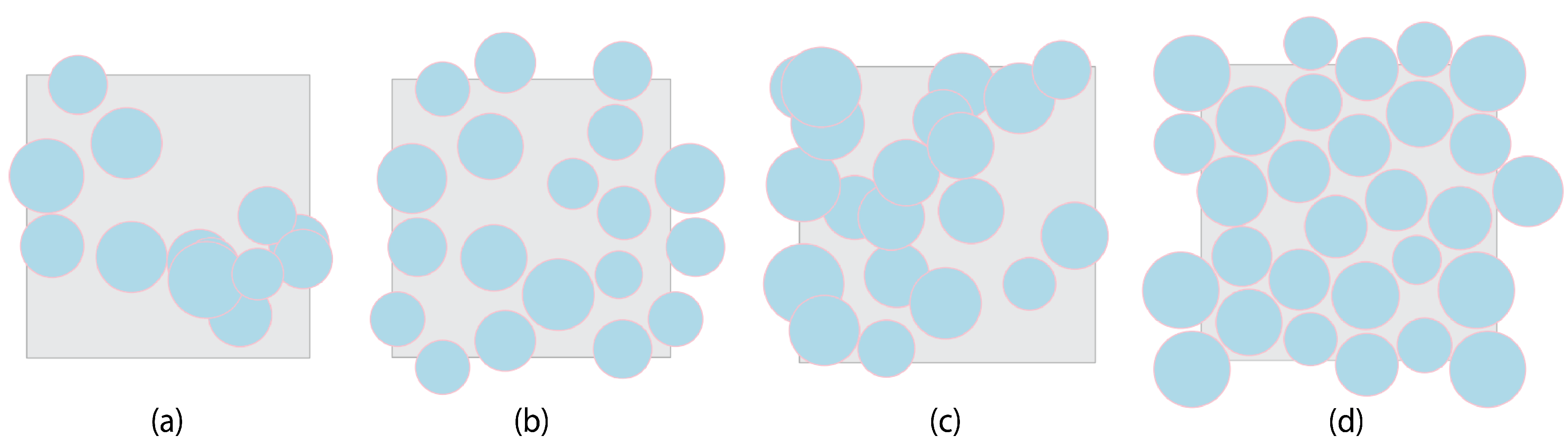
4.1. Microstructure Generation
| Algorithm 1 Pseudocode for generating microstructure |
|
4.2. Periodic Boundary Conditions (PBCs) and Displacement Boundary Conditions
4.3. Constitutive Models and Discretization of Fiber, Matrix, and Interface

4.4. Loading Cases and Steps
4.5. RVE Size Validation
4.6. Solver, Postprocessing, and Implementation
5. Full Factorial DOE and Monte Carlo Simulation for Virtual Tests
6. RVE Model Validation
6.1. Efficiency and Execution Time of the Algorithm for RVE Model Generation and Analysis
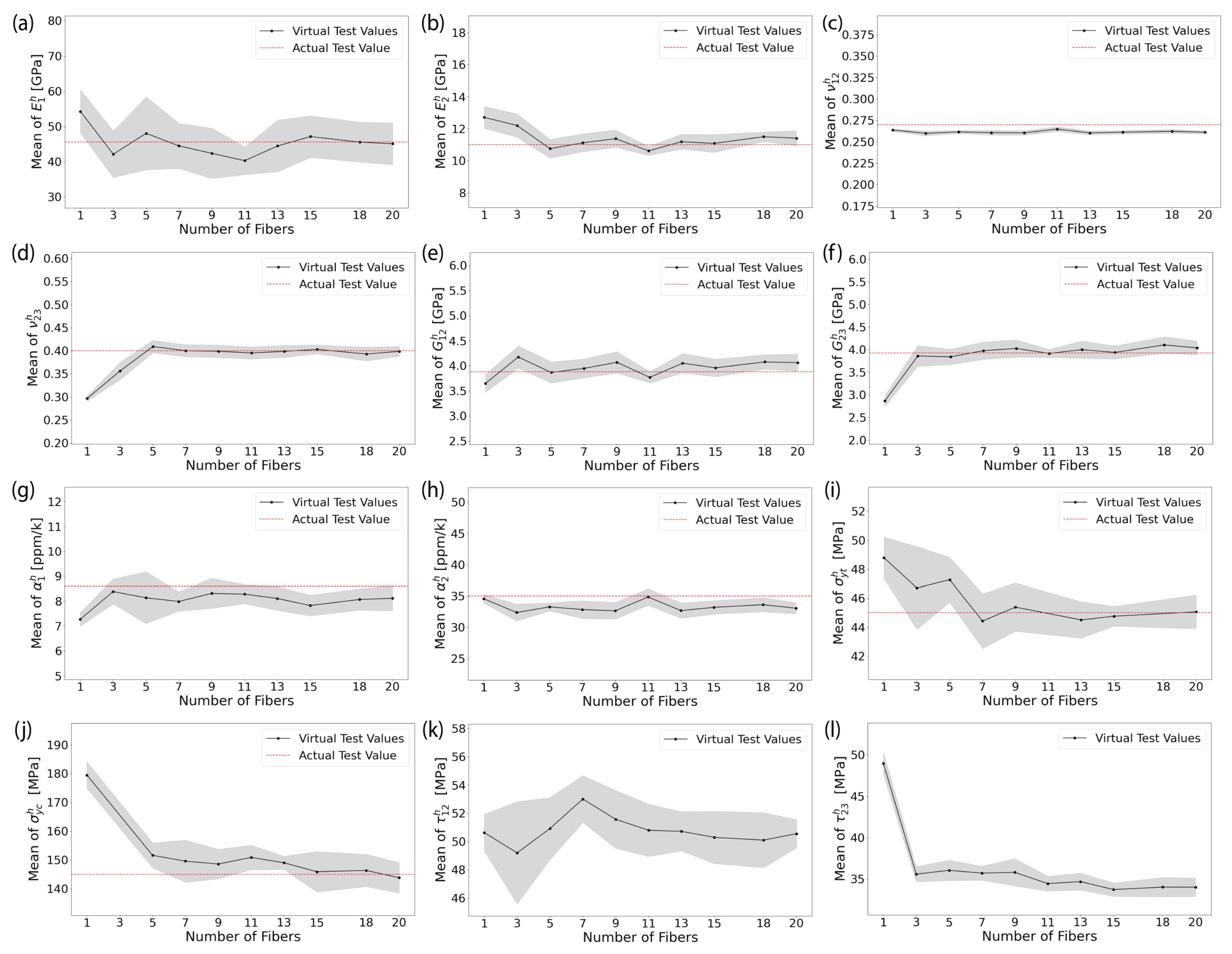
6.2. Optimum RVE Size and Model Prediction Validity from the Perspective of Homogenized Elastic Properties and Damage Initiation Strengths
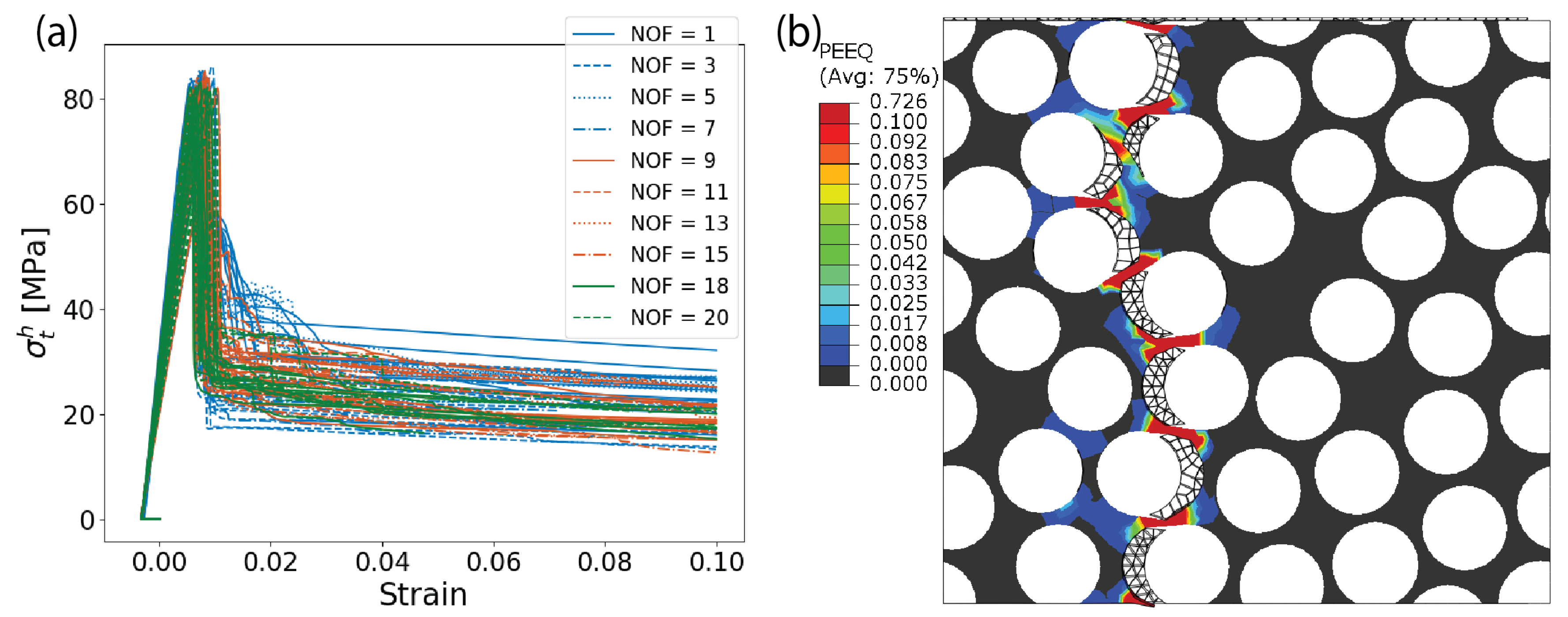
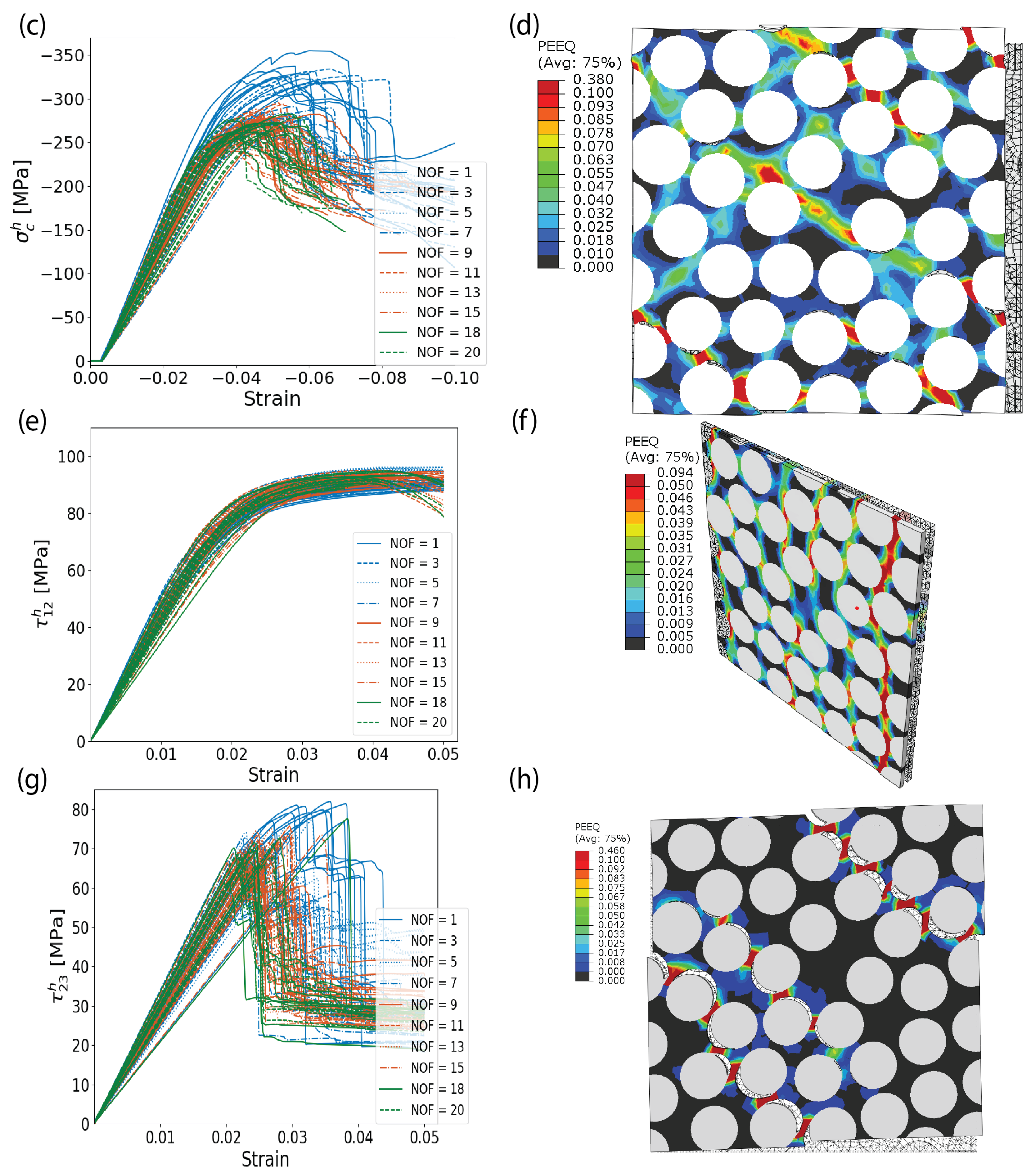
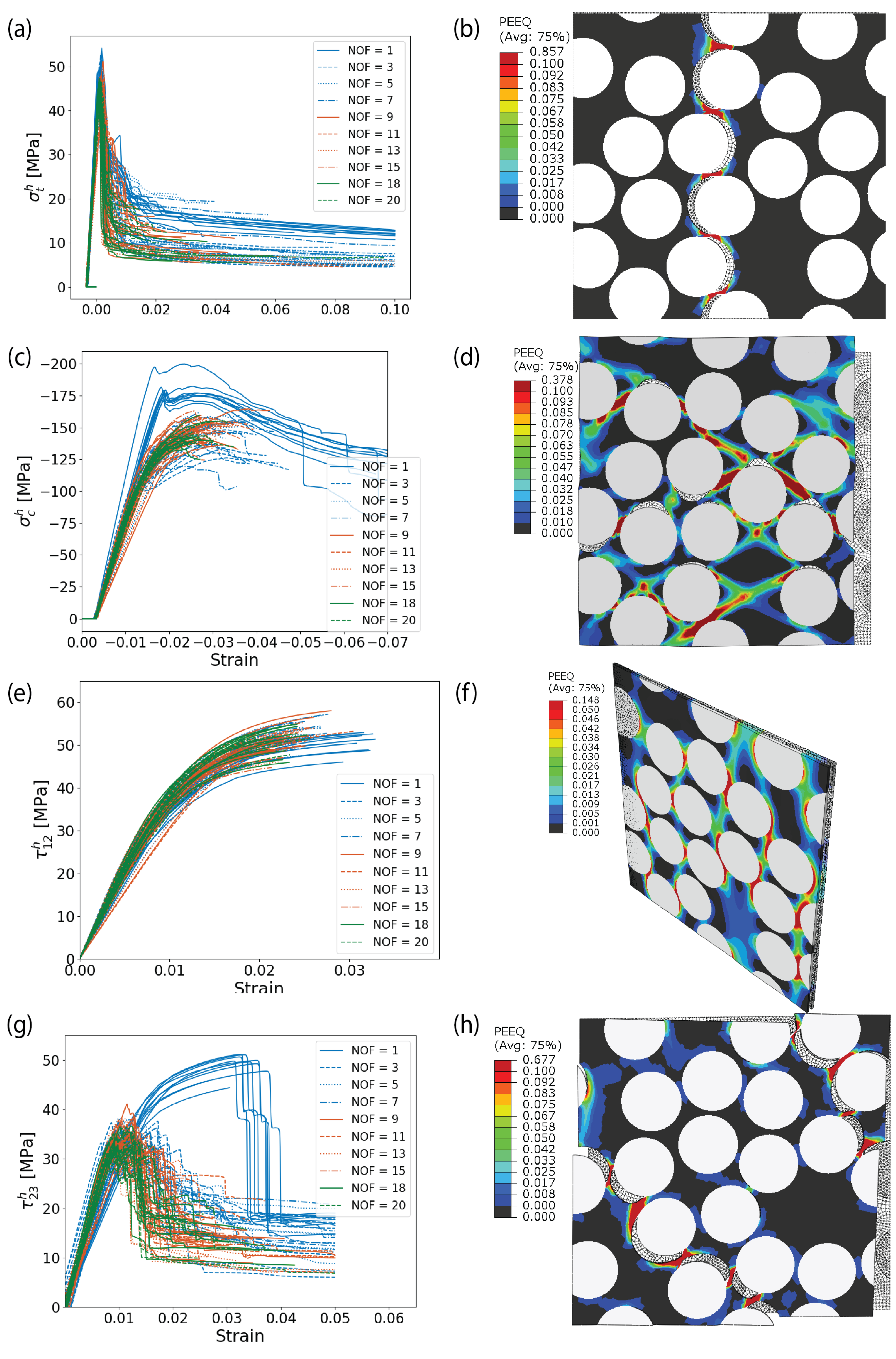
6.3. Models’ Validity in Predicting Failure Modes and Locus
7. The Effect of vf on the Size of RVE across Various FRP Types
8. The Effect of vf on the Reliability and Predictability of Homogenized Elastic Properties and Damage Initiation Strengths across Various FRP Types
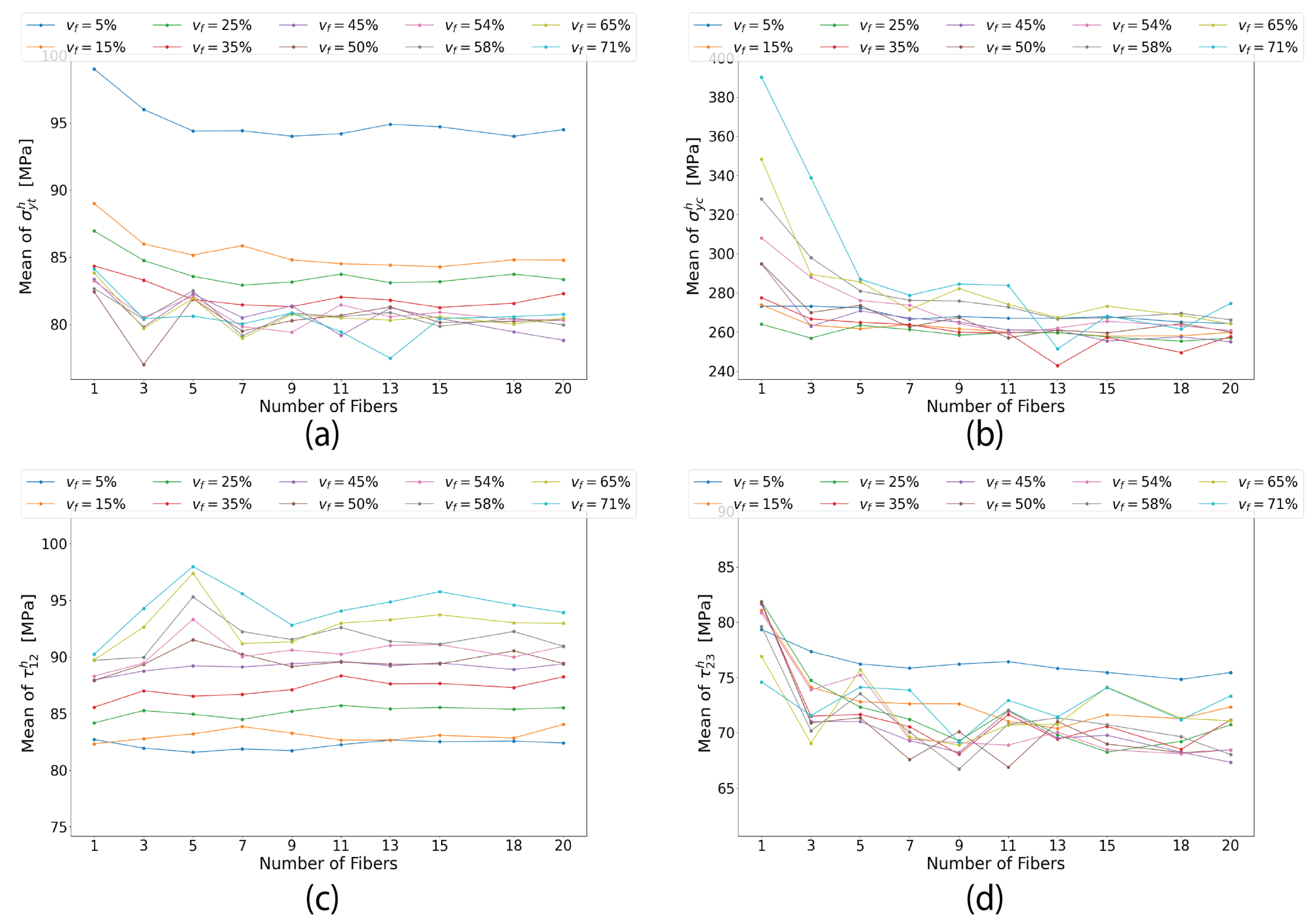
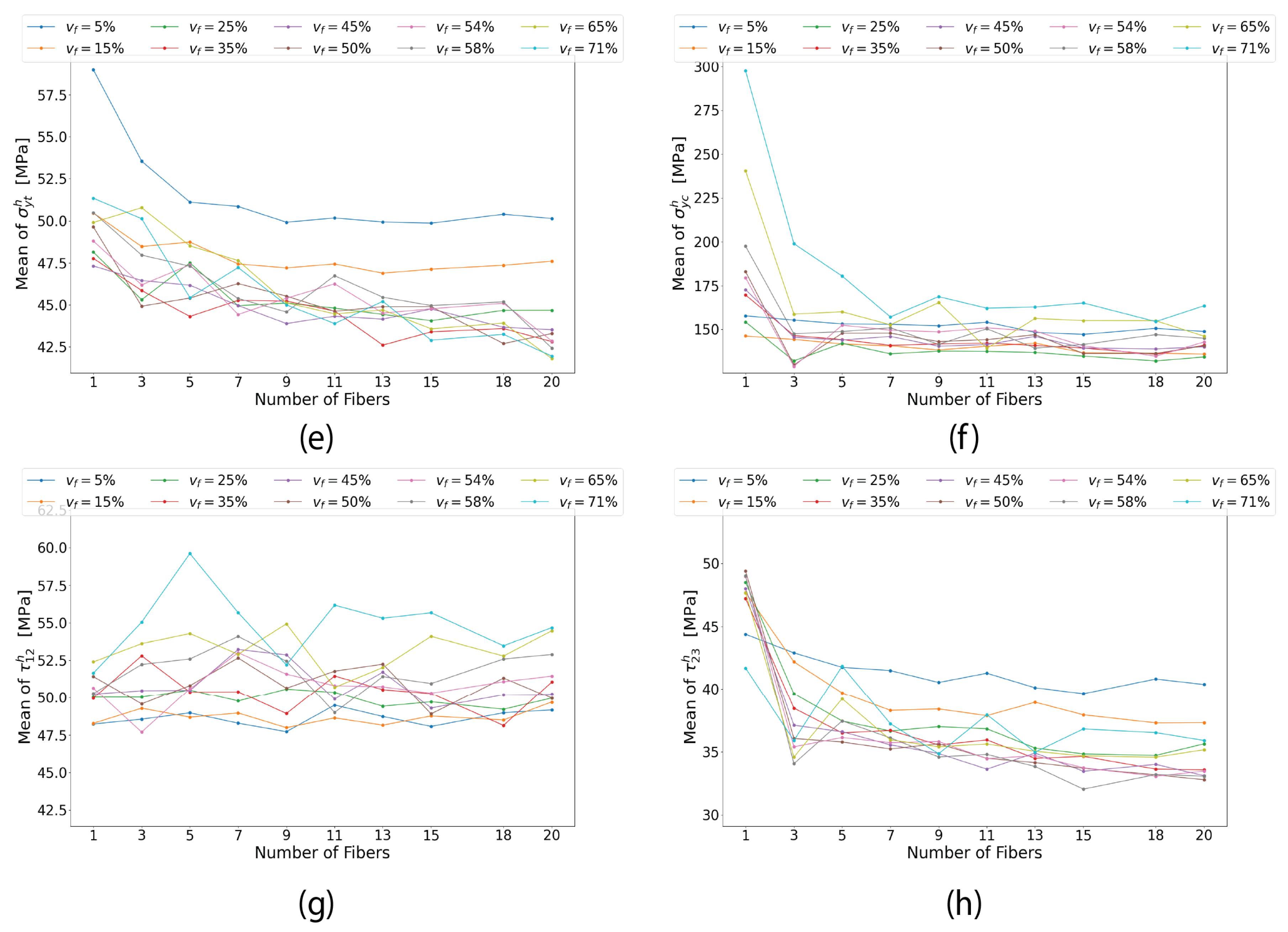
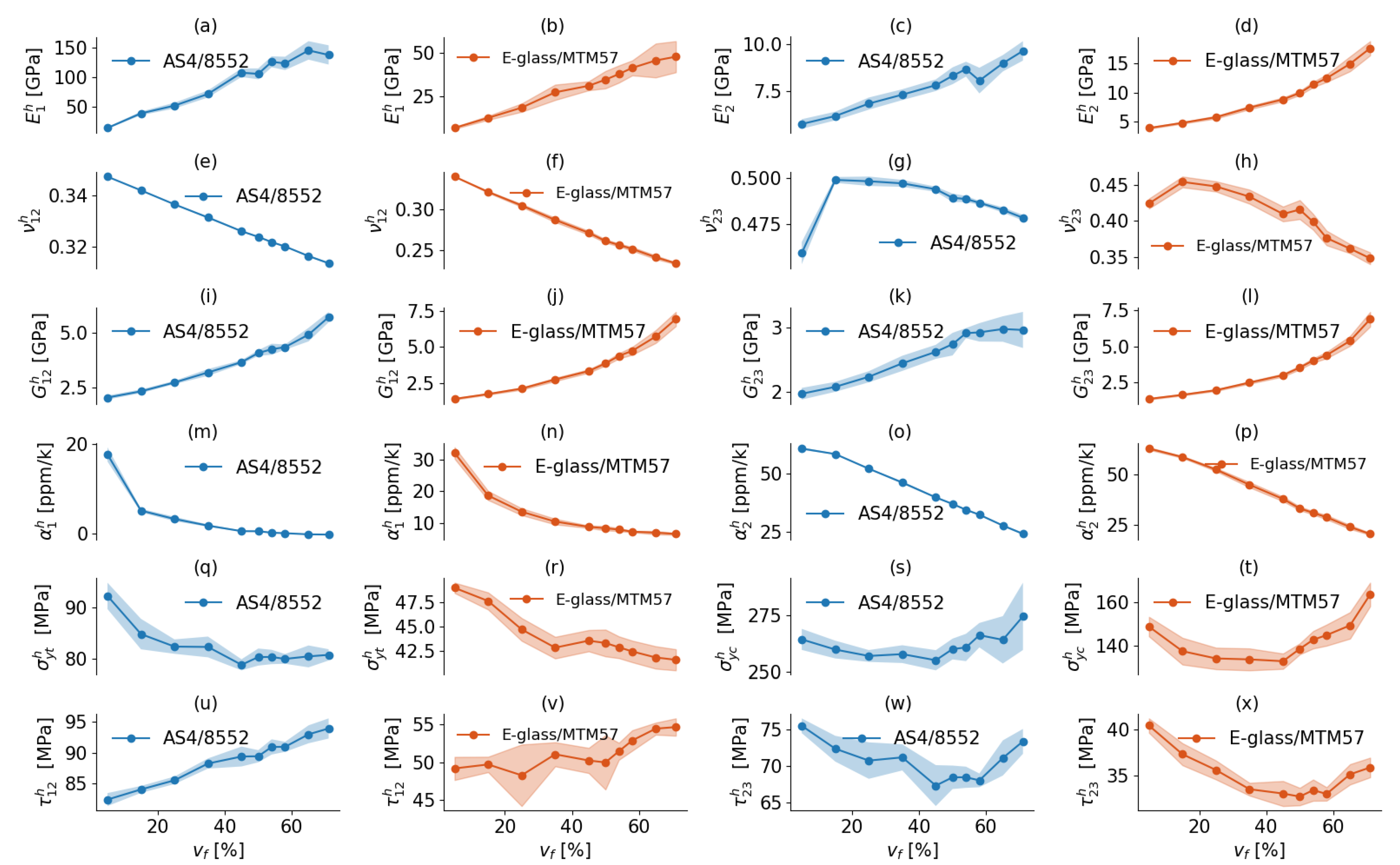
8.1. Effect of on the Predicted Properties
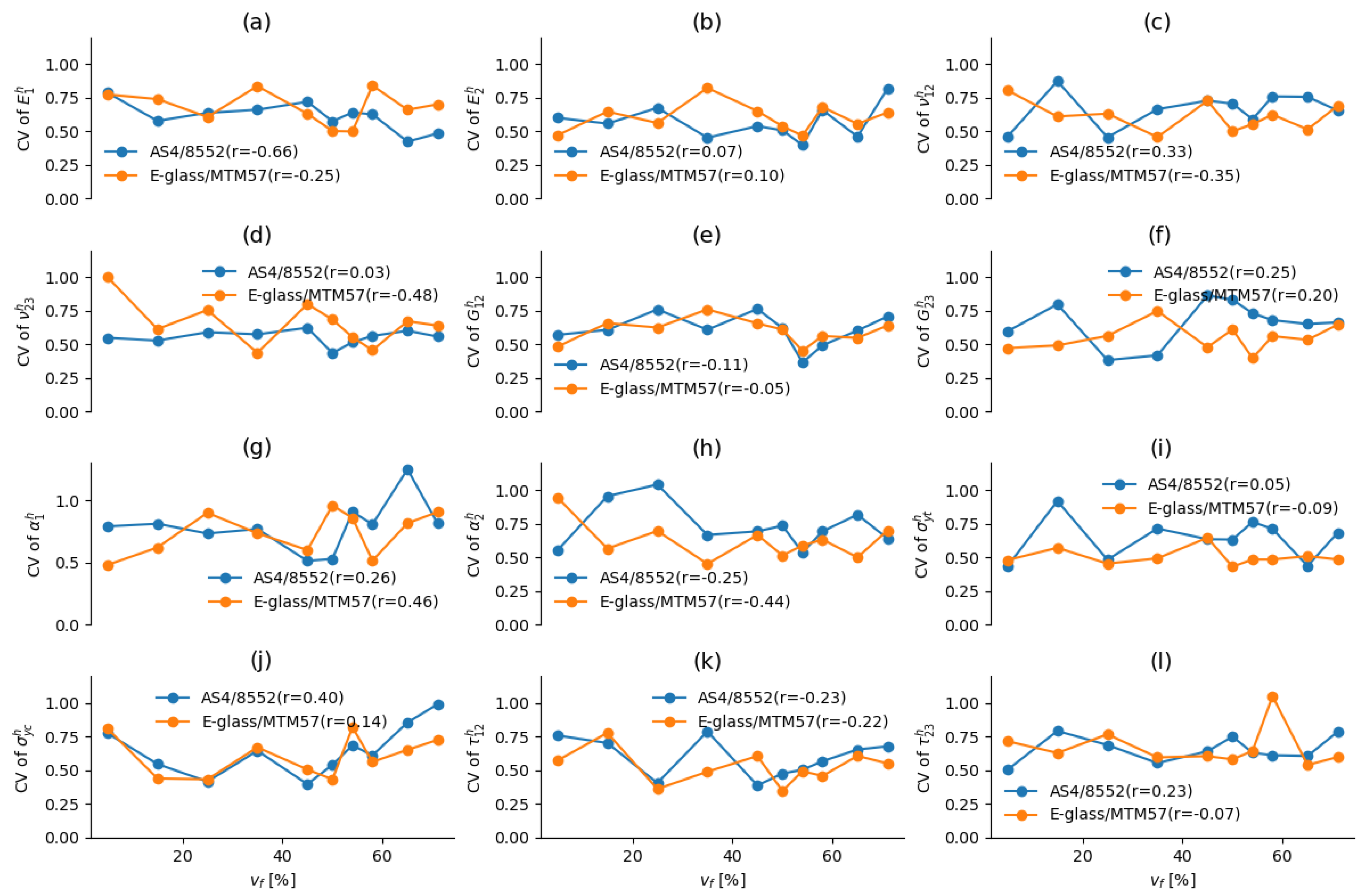
8.2. Effect of on the CV of the Predicted Properties
9. Conclusions
- The modified algorithm based on a constrained optimization formulation exhibited exceptional performance regarding convergence speed and jamming limit, which reached . It took less than 5 minutes on average to generate a feasible microstructure of size with a of , which is lower than the time required by the original algorithm (18 minutes) to generate a microstructure with the same size and . This is highly beneficial for uncertainty analysis using virtual testing, particularly when many microstructures need to be generated.
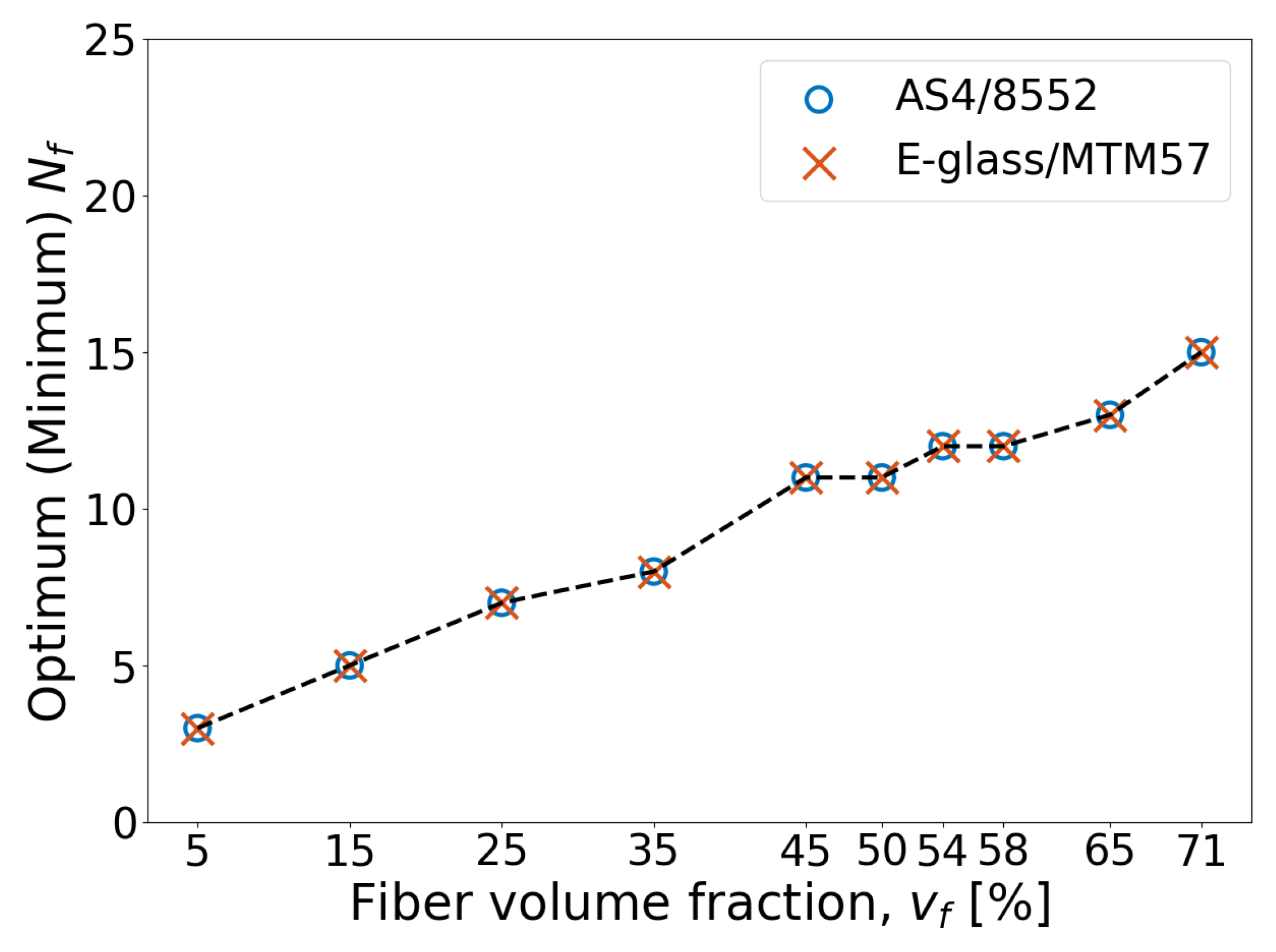
- Increasing leads to a concurrent increase in the minimum or optimal size of the RVE (i.e., ) required to ensure the convergence of homogenized mechanical properties. This outcome is explicable by the fact that an increase in necessitates a larger RVE with a higher to encompass the full spectrum of irregularities, such as fiber clustering and resin-rich areas, which have a pronounced influence on the predicted stress distribution and mechanical properties. Conversely, when is extremely low, it seems that a unit cell model in some scenarios or a model of two or three fibers suffices to include the full spectrum of irregularities.
- Increasing in fiber-reinforced polymers (FRPs) accentuates the influence of fiber properties on the composite’s properties. In cases like UD AS4/8552 and E-glass/MTM57, the fibers’ stiffnesses () surpassed that of the matrix, leading to an overall increase in the stiffness of the composite. Conversely, the Poisson’s ratios and thermal expansion coefficients of the fibers were lower than those of the matrix, causing a decrease in these properties for the FRPs with increasing .
- Regarding damage initiation strengths, increasing in UD AS4/8552 and E-glass/MTM57 resulted in higher longitudinal tensile and shear strengths, but lower transverse tensile strength due to reduced matrix areas available to resist loads, leading to the creation of stress concentration areas and, consequently, a lower load carrying capacity. Transverse compressive and shear strengths decreased initially with the increase in up to a specific threshold (), but increasing beyond this threshold corresponded to an increase in these strengths. This could be attributed to the formation of fiber clusters contributing to resisting the compressive load in the transverse direction.
- While indeed had a direct influence on the values of homogenized elastic properties and damage initiation strengths, it did not appear to have a distinct or significant effect on the reliability and predictability of these properties. This conclusion was substantiated by the low values of the correlation coefficient (r) and the observed fluctuations in the value of the CV of the normalized properties as changed.
Author Contributions
Funding
Institutional Review Board Statement
Informed Consent Statement
Data Availability Statement
Acknowledgments
Conflicts of Interest
References
- Maiti, S.; Islam, M.R.; Uddin, M.A.; Afroj, S.; Eichhorn, S.J.; Karim, N. Sustainable Fiber-Reinforced Composites: A Review. Adv. Sustain. Syst. 2022, 6, 2200258. [Google Scholar] [CrossRef]
- Zhou, X.Y.; Qian, S.Y.; Wang, N.W.; Xiong, W.; Wu, W.Q. A review on stochastic multiscale analysis for FRP composite structures. Compos. Struct. 2022, 284, 115132. [Google Scholar] [CrossRef]
- Mesogitis, T.; Skordos, A.; Long, A. Uncertainty in the manufacturing of fibrous thermosetting composites: A review. Compos. Part Appl. Sci. Manuf. 2014, 57, 67–75. [Google Scholar] [CrossRef]
- Abdollahiparsa, H.; Shahmirzaloo, A.; Teuffel, P.; Blok, R. A review of recent developments in structural applications of natural fiber-Reinforced composites (NFRCs). Compos. Adv. Mater. 2023, 32, 26349833221147540. [Google Scholar] [CrossRef]
- Hegde, S.; Satish Shenoy, B.; Chethan, K. Review on carbon fiber reinforced polymer (CFRP) and their mechanical performance. Mater. Today Proc. 2019, 19, 658–662. [Google Scholar] [CrossRef]
- Alam, P.; Mamalis, D.; Robert, C.; Floreani, C.; Ó Brádaigh, C.M. The fatigue of carbon fibre reinforced plastics—A review. Compos. Part Eng. 2019, 166, 555–579. [Google Scholar] [CrossRef]
- Cai, R.; Jin, T. The effect of microstructure of unidirectional fibre-reinforced composites on mechanical properties under transverse loading: A review. J. Reinf. Plast. Compos. 2018, 37, 1360–1377. [Google Scholar] [CrossRef]
- Okereke, M.I.; Akpoyomare, A.I.; Bingley, M.S. Virtual testing of advanced composites, cellular materials and biomaterials: A review. Compos. Part Eng. 2014, 60, 637–662. [Google Scholar] [CrossRef]
- Wan, L. Progressive Damage Mechanisms and Failure Predictions of Fibre-Reinforced Polymer Composites under Quasi-Static Loads Using the Finite Element and Discrete Element Methods. Ph.D. Thesis, The University of Edinburgh, Edinburgh, UK, 2020. [Google Scholar] [CrossRef]
- LLorca, J.; González, C.; Molina-Aldareguía, J.M.; Segurado, J.; Seltzer, R.; Sket, F.; Rodríguez, M.; Sádaba, S.; Muñoz, R.; Canal, L.P. Multiscale Modeling of Composite Materials: A Roadmap Towards Virtual Testing. Adv. Mater. 2011, 23, 5130–5147. [Google Scholar] [CrossRef]
- Kwon, Y.W.; Allen, D.H.; Talreja, R. (Eds.) Multiscale Modeling and Simulation of Composite Materials and Structures; Springer US: Boston, MA, USA, 2008. [Google Scholar] [CrossRef]
- Chowdhury, N.T.; Wang, J.; Chiu, W.K.; Yan, W. Predicting matrix failure in composite structures using a hybrid failure criterion. Compos. Struct. 2016, 137, 148–158. [Google Scholar] [CrossRef]
- Naya, F.; González, C.; Lopes, C.; Van Der Veen, S.; Pons, F. Computational micromechanics of the transverse and shear behavior of unidirectional fiber reinforced polymers including environmental effects. Compos. Part Appl. Sci. Manuf. 2017, 92, 146–157. [Google Scholar] [CrossRef]
- Naya, F.; Herráez, M.; Lopes, C.; González, C.; Van Der Veen, S.; Pons, F. Computational micromechanics of fiber kinking in unidirectional FRP under different environmental conditions. Compos. Sci. Technol. 2017, 144, 26–35. [Google Scholar] [CrossRef]
- Totry, E.; González, C.; LLorca, J. Failure locus of fiber-reinforced composites under transverse compression and out-of-plane shear. Compos. Sci. Technol. 2008, 68, 829–839. [Google Scholar] [CrossRef]
- Totry, E.; González, C.; LLorca, J. Prediction of the failure locus of C/PEEK composites under transverse compression and longitudinal shear through computational micromechanics. Compos. Sci. Technol. 2008, 68, 3128–3136. [Google Scholar] [CrossRef]
- González, C.; LLorca, J. Mechanical behavior of unidirectional fiber-reinforced polymers under transverse compression: Microscopic mechanisms and modeling. Compos. Sci. Technol. 2007, 67, 2795–2806. [Google Scholar] [CrossRef]
- Canal, L.P.; González, C.; Segurado, J.; LLorca, J. Intraply fracture of fiber-reinforced composites: Microscopic mechanisms and modeling. Compos. Sci. Technol. 2012, 72, 1223–1232. [Google Scholar] [CrossRef]
- Herráez, M.; Mora, D.; Naya, F.; Lopes, C.S.; González, C.; LLorca, J. Transverse cracking of cross-ply laminates: A computational micromechanics perspective. Compos. Sci. Technol. 2015, 110, 196–204. [Google Scholar] [CrossRef]
- Canal Casado, L.P. Experimental and Computational Micromechanical Study of Fiber-Reinforced Polymers. Ph.D. Thesis, Canales y Puertos (UPM), Madrid, Spain, 2011. [Google Scholar] [CrossRef]
- Vaughan, T.J. Micromechanical Modelling of Damage and Failure in Fibre Reinforced Composites under Loading in the Transverse Plane. Ph.D. Thesis, University of Limerick, Limerick, Ireland, 2011. [Google Scholar]
- Naderi, M.; Iyyer, N.; Chandrashekhara, K. Micromechanisms of Failure and Damage Evolution in Low-Thickness Composite Laminates Under Tensile Loading. J. Fail. Anal. Prev. 2019, 19, 1761–1773. [Google Scholar] [CrossRef]
- Chamis, C.C. Probabilistic simulation of multi-scale composite behavior. Theor. Appl. Fract. Mech. 2004, 41, 51–61. [Google Scholar] [CrossRef]
- Sakata, S.i.; Torigoe, I. A successive perturbation-based multiscale stochastic analysis method for composite materials. Finite Elem. Anal. Des. 2015, 102–103, 74–84. [Google Scholar] [CrossRef]
- Thapa, M.; Mulani, S.B.; Walters, R.W. Stochastic multi-scale modeling of carbon fiber reinforced composites with polynomial chaos. Compos. Struct. 2019, 213, 82–97. [Google Scholar] [CrossRef]
- Kanouté, P.; Boso, D.P.; Chaboche, J.L.; Schrefler, B.A. Multiscale methods for composites: A Review. Arch. Comput. Methods Eng. 2009, 16, 31–75. [Google Scholar] [CrossRef]
- Christoff, B.G.; Almeida, J.H.; Ribeiro, M.L.; Maciel, M.M.; Guedes, R.M.; Tita, V. Multiscale modelling of composite laminates with voids through the direct FE2 method. Theor. Appl. Fract. Mech. 2024, 131, 104424. [Google Scholar] [CrossRef]
- Hill, R. Elastic properties of reinforced solids: Some theoretical principles. J. Mech. Phys. Solids 1963, 11, 357–372. [Google Scholar] [CrossRef]
- Liu, K.C.; Ghoshal, A. Validity of random microstructures simulation in fiber-reinforced composite materials. Compos. Part Eng. 2014, 57, 56–70. [Google Scholar] [CrossRef]
- Swaminathan, S.; Ghosh, S.; Pagano, N.J. Statistically Equivalent Representative Volume Elements for Unidirectional Composite Microstructures: Part I - Without Damage. J. Compos. Mater. 2006, 40, 583–604. [Google Scholar] [CrossRef]
- Gitman, I.M.; Askes, H.; Sluys, L.J. Representative volume: Existence and size determination. Eng. Fract. Mech. 2007, 74, 2518–2534. [Google Scholar] [CrossRef]
- Islam, F.; Joannès, S.; Bunsell, A.; Laiarinandrasana, L. Adaptation of Weibull analysis to represent strength behaviour of brittle fibres. In Proceedings of the ICCM 22-22nd International Conference on Composite Materials, Melbourne, Australia, 11–16 August 2019. [Google Scholar]
- Costa, d.L.; Loiola, R.; Monteiro, S. Diameter dependence of tensile strength by Weibull analysis: Part I bamboo fiber. Matéria (Rio de Janeiro) 2010, 15, 110–116. [Google Scholar] [CrossRef]
- Dessalegn, Y.; Singh, B.; Vuure, v.A.W.; Badruddin, I.A.; Beri, H.; Hussien, M.; Ahmed, G.M.S.; Hossain, N. Investigation of Bamboo Fibrous Tensile Strength Using Modified Weibull Distribution. Materials 2022, 15, 5016. [Google Scholar] [CrossRef]
- Wang, F.; Shao, J. Modified Weibull Distribution for Analyzing the Tensile Strength of Bamboo Fibers. Polymers 2014, 6, 3005–3018. [Google Scholar] [CrossRef]
- Sayeed, M.M.A.; Paharia, A. Optimisation of the surface treatment of jute fibres for natural fibre reinforced polymer composites using Weibull analysis. J. Text. Inst. 2019, 110, 1588–1595. [Google Scholar] [CrossRef]
- Swolfs, Y.; Gorbatikh, L.; Verpoest, I. Fibre hybridisation in polymer composites: A review. Compos. Part Appl. Sci. Manuf. 2014, 67, 181–200. [Google Scholar] [CrossRef]
- Liaw, D.; Singhal, S.; Murthy, P.; Chamis, C.C. Quantification of uncertainties in Composites. In Proceedings of the 34th Structures, Structural Dynamics, and Materials Conference, La Jolla, CA, USA, 19–22 April 1993. [Google Scholar] [CrossRef]
- Sriramula, S.; Chryssanthopoulos, M.K. Quantification of uncertainty modelling in stochastic analysis of FRP composites. Compos. Part Appl. Sci. Manuf. 2009, 40, 1673–1684. [Google Scholar] [CrossRef]
- Naya Montáns, F. Prediction of Mechanical Properties of Unidirectional FRP Plies at Different Environmental Conditions by Means of Computational Micromechanics. Ph.D. Thesis, E.T.S.I. Caminos, Canales y Puertos (UPM), Madrid, Spain, 2017. [Google Scholar]
- Bechtold, G.; Ye, L. Influence of fibre distribution on the transverse flow permeability in fibre bundles. Compos. Sci. Technol. 2003, 63, 2069–2079. [Google Scholar] [CrossRef]
- Rintoul, M.D.; Torquato, S. Reconstruction of the Structure of Dispersions. J. Colloid Interface Sci. 1997, 186, 467–476. [Google Scholar] [CrossRef]
- Feder, J. Random sequential adsorption. J. Theor. Biol. 1980, 87, 237–254. [Google Scholar] [CrossRef]
- Tory, E.M.; Jodrey, W.S.; Pickard, D.K. Simulation of random sequential adsorption: Efficient methods and resolution of conflicting results. J. Theor. Biol. 1983, 102, 439–445. [Google Scholar] [CrossRef]
- Buryachenko, V.; Pagano, N.; Kim, R.; Spowart, J. Quantitative description and numerical simulation of random microstructures of composites and their effective elastic moduli. Int. J. Solids Struct. 2003, 40, 47–72. [Google Scholar] [CrossRef]
- Oh, J.H.; Jin, K.K.; Ha, S.K. Interfacial Strain Distribution of a Unidirectional Composite with Randomly Distributed Fibers under Transverse Loading. J. Compos. Mater. 2006, 40, 759–778. [Google Scholar] [CrossRef]
- Bulsara, V.N.; Talreja, R.; Qu, J. Damage initiation under transverse loading of unidirectional composites with arbitrarily distributed ®bers. Compos. Sci. Technol. 1999, 59, 673–682. [Google Scholar] [CrossRef]
- Yang, L.; Yan, Y.; Ran, Z.; Liu, Y. A new method for generating random fibre distributions for fibre reinforced composites. Compos. Sci. Technol. 2013, 76, 14–20. [Google Scholar] [CrossRef]
- Vaughan, T.; McCarthy, C. A combined experimental–numerical approach for generating statistically equivalent fibre distributions for high strength laminated composite materials. Compos. Sci. Technol. 2010, 70, 291–297. [Google Scholar] [CrossRef]
- Ghossein, E.; Lévesque, M. A fully automated numerical tool for a comprehensive validation of homogenization models and its application to spherical particles reinforced composites. Int. J. Solids Struct. 2012, 49, 1387–1398. [Google Scholar] [CrossRef]
- Herráez, M.; Segurado, J.; González, C.; Lopes, C. A microstructures generation tool for virtual ply property screening of hybrid composites with high volume fractions of non-circular fibers–VIPER. Compos. Part Appl. Sci. Manuf. 2020, 129, 105691. [Google Scholar] [CrossRef]
- Pathan, M.; Tagarielli, V.; Patsias, S.; Baiz-Villafranca, P. A new algorithm to generate representative volume elements of composites with cylindrical or spherical fillers. Compos. Part Eng. 2017, 110, 267–278. [Google Scholar] [CrossRef]
- Herráez, M.; Fernández, A.; Lopes, C.S.; González, C. Strength and toughness of structural fibres for composite material reinforcement. Philos. Trans. R. Soc. Math. Phys. Eng. Sci. 2016, 374, 20150274. [Google Scholar] [CrossRef]
- Shirasu, K.; Goto, K.; Naito, K. Microstructure-elastic property relationships in carbon fibers: A nanoindentation study. Compos. Part Eng. 2020, 200, 108342. [Google Scholar] [CrossRef]
- Hawthorne, H.M.; Teghtsoonian, E. Axial compression fracture in carbon fibres. J. Mater. Sci. 1975, 10, 41–51. [Google Scholar] [CrossRef]
- Herráez, M.; Bergan, A.; Lopes, C.; González, C. Computational micromechanics model for the analysis of fiber kinking in unidirectional fiber-reinforced polymers. Mech. Mater. 2020, 142, 103299. [Google Scholar] [CrossRef]
- The transverse compression of anisotropic fibre monofilaments. Proc. R. Soc. Lond. Ser. Math. Phys. Sci. 1965, 285, 275–286. [CrossRef]
- Phoenix, S.; Skelton, J. Transverse Compressive Moduli and Yield Behavior of Some Orthotropic, High-Modulus Filaments. Text. Res. J. 1974, 44, 934–940. [Google Scholar] [CrossRef]
- Kaddour, A.; Hinton, M. Input data for test cases used in benchmarking triaxial failure theories of composites. J. Compos. Mater. 2012, 46, 2295–2312. [Google Scholar] [CrossRef]
- Rodríguez, M.; Molina-Aldareguía, J.; González, C.; LLorca, J. Determination of the mechanical properties of amorphous materials through instrumented nanoindentation. Acta Mater. 2012, 60, 3953–3964. [Google Scholar] [CrossRef]
- Herráez, M.; Naya, F.; González, C.; Monclús, M.; Molina, J.; Lopes, C.S.; LLorca, J. Microscale Characterization Techniques of Fibre-Reinforced Polymers. In The Structural Integrity of Carbon Fiber Composites: Fifty Years of Progress and Achievement of the Science, Development, and Applications; Beaumont, P.W.R., Soutis, C., Hodzic, A., Eds.; Springer International Publishing: Cham, Switzerland, 2017; pp. 283–299. [Google Scholar] [CrossRef]
- Kelly, A.; Tyson, W.R. Tensile properties of fibre-reinforced metals: Copper/tungsten and copper/molybdenum. J. Mech. Phys. Solids 1965, 13, 329–350. [Google Scholar] [CrossRef]
- Kim, J.K.; Baillie, C.; Mai, Y.W. Interfacial debonding and fibre pull-out stresses. J. Mater. Sci. 1992, 27, 3143–3154. [Google Scholar] [CrossRef]
- Miller, B.; Muri, P.; Rebenfeld, L. A microbond method for determination of the shear strength of a fiber/resin interface. Compos. Sci. Technol. 1987, 28, 17–32. [Google Scholar] [CrossRef]
- Medina M, C.; Molina-Aldareguía, J.M.; González, C.; Melendrez, M.F.; Flores, P.; LLorca, J. Comparison of push-in and push-out tests for measuring interfacial shear strength in nano-reinforced composite materials. J. Compos. Mater. 2016, 50, 1651–1659. [Google Scholar] [CrossRef]
- Ogihara, S.; Koyanagi, J. Investigation of combined stress state failure criterion for glass fiber/epoxy interface by the cruciform specimen method. Compos. Sci. Technol. 2010, 70, 143–150. [Google Scholar] [CrossRef]
- Byrd, R.H.; Lu, P.; Nocedal, J.; Zhu, C. A Limited Memory Algorithm for Bound Constrained Optimization. Siam J. Sci. Comput. 1995, 16, 1190–1208. [Google Scholar] [CrossRef]
- Drucker, D.C.; Prager, W. Soil Mechanics and Plastic Analysis or Limit Design. Q. Appl. Math. 1952, 10, 157–165. [Google Scholar] [CrossRef]
- Dassault Systèmes. Abaqus 2021 Documentation; Dassault Systèmes: Vélizy-Villacoublay, France, 2021. [Google Scholar]
- Camanho, P.P.; Davila, C.G. Mixed-Mode Decohesion Finite Elements for the Simulation of Delamination in Composite Materials; Technical report; Document ID: 20020053651; NASA Langley Research Center: Hampton, VA, USA, 2002. [Google Scholar]
- Turon, A.; Camanho, P.P.; Costa, J.; Dávila, C.G. A damage model for the simulation of delamination in advanced composites under variable-mode loading. Mech. Mater. 2006, 38, 1072–1089. [Google Scholar] [CrossRef]
- Turon, A.; Camanho, P.P.; Costa, J.; Renart, J. Accurate simulation of delamination growth under mixed-mode loading using cohesive elements: Definition of interlaminar strengths and elastic stiffness. Compos. Struct. 2010, 92, 1857–1864. [Google Scholar] [CrossRef]
- Rocha, R.; Campilho, R.; Silva, F. Validation of advanced numerical techniques for the strength prediction of adhesively-bonded joints. Procedia Manuf. 2017, 13, 43–50. [Google Scholar] [CrossRef]
- Marlett, K. Hexcel 8552 AS4 Unidirectional Prepreg at 190 gsm & 35% RC Qualification Material Property Data Report FAA Special Project Number SP4614WI-Q NCAMP Test Report Number: CAM-RP-2010-002 Rev.; Technical report; Wichita State University: Wichita, KS, USA, 2011. [Google Scholar]
- Kumbhare, N.; Moheimani, R.; Dalir, H. Analysis of Composite Structures in Curing Process for Shape Deformations and Shear Stress: Basis for Advanced Optimization. J. Compos. Sci. 2021, 5, 63. [Google Scholar] [CrossRef]
- Kappel, E. On thermal-expansion properties of more-orthotropic prepreg laminates with and without interleaf layers. Compos. Part Open Access 2020, 3, 100059. [Google Scholar] [CrossRef]
- Ahamed, J.; Joosten, M.; Callus, P.; John, S.; Wang, C.H. Ply-interleaving technique for joining hybrid carbon/glass fibre composite materials. Compos. Part A Appl. Sci. Manuf. 2016, 84, 134–146. [Google Scholar] [CrossRef]
- Okutan Baba, B. Behavior of Pin-loaded Laminated Composites. Exp. Mech. 2006, 46, 589–600. [Google Scholar] [CrossRef]
- Pinho, S.; Darvizeh, R.; Robinson, P.; Schuecker, C.; Camanho, P. Material and structural response of polymer-matrix fibre-reinforced composites. J. Compos. Mater. 2012, 46, 2313–2341. [Google Scholar] [CrossRef]


| Fiber | [GPa] | [GPa] | [GPa] | [GPa] | [ppm/K] | [ppm/K] | [MPa] | [MPa] | |
|---|---|---|---|---|---|---|---|---|---|
| AS4 | 231 | 12.9 | 11.3 | 4.45 | 0.3 | −0.7 | 12 | 4000 | 3500 |
| E-Glass | 74 | 74 | 30.8 | 30.8 | 0.2 | 4.9 | 4.9 | 2150 | 1450 |
| Epoxy | [GPa] | [ppm/K] | [MPa] | [MPa] | [MPa] | [J/m2] | [°] | |
|---|---|---|---|---|---|---|---|---|
| 8552 | 5.1 ± 0.3 | 0.35 | 52 | 120 | 176 ± 3 | 180 | 90 | 29 ± 1 |
| MTM57 | 3.5 ± 0.2 | 0.35 | 58 | ≥75 | 105 ± 5 | - | - | - |
| Interface | [MPa] | [MPa] | [J/m2] | [J/m2] | [GPa/m] | [GPa/m] |
|---|---|---|---|---|---|---|
| AS4/epoxy | 57 | 85 | 7 | 80 | 100 | 100 |
| E-glass/epoxy | 50 | 75 | 2 | 10 | 100 | 100 |
| Factors | Levels |
|---|---|
| [%] | 10 Levels (5, 15, 25, 35, 45, 50, 54, 58, 65, 71) |
| RVE size, | 10 Levels (1, 3, 5, 7, 9, 11, 13, 15, 18, 20) |
| Composite Type | [GPa] | [GPa] | [GPa] | [GPa] | [ppm/K] | [ppm/K] | [MPa] | [MPa] | ||
|---|---|---|---|---|---|---|---|---|---|---|
| AS4/8552 | 141 | 9.2 | 0.302 | 0.49 | 5.2 | 3.19 | 0~−0.8 | 31.2 | 81 | 260 |
| E-glass/MTM57 | 45.6 | 11 | 0.27 | 0.4 | 3.88 | 3.93 | 8.6 | 35 | 45 | 145 |
Disclaimer/Publisher’s Note: The statements, opinions and data contained in all publications are solely those of the individual author(s) and contributor(s) and not of MDPI and/or the editor(s). MDPI and/or the editor(s) disclaim responsibility for any injury to people or property resulting from any ideas, methods, instructions or products referred to in the content. |
© 2024 by the authors. Licensee MDPI, Basel, Switzerland. This article is an open access article distributed under the terms and conditions of the Creative Commons Attribution (CC BY) license (https://creativecommons.org/licenses/by/4.0/).
Share and Cite
Alhaddad, W.; He, M.; Halabi, Y.; Almajhali, K.Y.M. Influence of Fiber Volume Fraction on the Predictability of UD FRP Ply Behavior: A Validated Micromechanical Virtual Testing Approach. Materials 2024, 17, 4736. https://doi.org/10.3390/ma17194736
Alhaddad W, He M, Halabi Y, Almajhali KYM. Influence of Fiber Volume Fraction on the Predictability of UD FRP Ply Behavior: A Validated Micromechanical Virtual Testing Approach. Materials. 2024; 17(19):4736. https://doi.org/10.3390/ma17194736
Chicago/Turabian StyleAlhaddad, Wael, Minjuan He, Yahia Halabi, and Khalil Yahya Mohammed Almajhali. 2024. "Influence of Fiber Volume Fraction on the Predictability of UD FRP Ply Behavior: A Validated Micromechanical Virtual Testing Approach" Materials 17, no. 19: 4736. https://doi.org/10.3390/ma17194736
APA StyleAlhaddad, W., He, M., Halabi, Y., & Almajhali, K. Y. M. (2024). Influence of Fiber Volume Fraction on the Predictability of UD FRP Ply Behavior: A Validated Micromechanical Virtual Testing Approach. Materials, 17(19), 4736. https://doi.org/10.3390/ma17194736