2.1. Metabolism and Heat Exchange
A part of the energy generated by the human body is devoted to its functioning; the rest is released to the environment. The intensity of these changes depends on [
20]: human metabolism, thermal insulation of clothing and the microclimate.
Human metabolism determines several processes occurring within an organism as a result of chemical reactions and is a source of heat in a human body [
20].
Balanced heat flux density can be converted into heat flux with a known surface area of the human skin. There are many formulas describing the relationship between surface area, body weight and human height—an example is the Haycock Formula.
The metabolic rate is most commonly linked to physical activity [
20], and it can be determined based on a set norm [
21]. The efficiency coefficient η = (17–25)%, which gives on average η = 20%. The perceived thermal comfort is determined by CT = (37 ± 0.3) °C and a skin temperature of about 33 °C [
20]. During extravehicular activity, it is assumed that for 7 h of work, the average metabolic rate does not exceed 300 W/m
2, and for 1 h of work, it does not exceed 470 W/m
2. Work under extreme conditions is permissible for 15 min, with the maximal rate of 600 W/m
2 [
8]. In laboratory research, the highest metabolic rate recorded was 880 W/m
2, while during the Apollo mission to the Moon, the lowest rate was at 144 W/m
2 [
22].
Thermal conductivity is a process of energy exchange between particles not undergoing macroscopic transformations. The base description is given by Fourier’s law. Space suits are constructions comprising multiple curves, described at any point by a variable radius. Therefore, conduction is described for a n-layered construction with variable curves in relation to the length unit [
23].
Heat radiation occurs from the suit’s surface (gray body) to the environment. The Stefan–Boltzmann law is described by the following equation [
20]:
The aim of the simulation is the assessment of the thermal insulation of the space suit during prolonged exposure to the extreme conditions in outer space. In this case, the steady-state conditions might be adapted for simplification. The equation of the thermal conductivity state is as follows [
24]:
The state variable in thermal conductivity issues is the temperature [
20,
25,
26]. It creates a state area since it is possible to be determined at every point of the suit.
2.2. Numerical Modeling
Two numerical models were analyzed in Ansys Workbench software (Ansys Workbench v. 2023)—the verification model under the simplified boundary conditions to assess the results’ credibility and the actual model with parameters similar to the outer space conditions. This enabled an assessment of the model’s quality and of the possible discrepancies.
The modeling of the structure was carried out with the Finite Element Method (FEM), and this process entailed the following steps [
27]:
Approximation—the application of the material data and geometrical conditions to ensure similarity between the model and the actual object.
Discretization—the transformation of a continuous mathematical model into a discrete model, divided into a finite number of elements.
The solution—the determination of the temperature area and the heat flux density.
Verification—the assessment of the quality of the obtained results, which will allow for the applied modifications.
The geometry of a finite element influences the quality of the obtained solution [
28,
29]. For the issues with directional changes, quadrilateral and hexagonal elements are proven to be more efficient, as their proportionality coefficients are notably larger than those of triangular elements. These help to significantly decrease the number of elements in the model, which also lessens the computational requirements for the computer [
30]. However, taking into account the sensitivity of the quadrilateral elements to the model’s geometry, it is impossible to obtain satisfactory results for more complex shapes.
There are no additional sources of heat in the adopted models. The mean value of the thermal conductivity coefficient is also assumed for the extreme temperatures. The ideal interaction between the layers‘ surfaces was introduced, which facilitates the examination of heat conduction only. The models, in addition to the material layers of the suit, also encompass the outer layers of the human skin. Thus, the aforementioned boundary condition is CT. Human skin temperature may differ due to environmental conditions and the heat flux penetrating the gear. The impact of the cooling factor within the space suit and of the radiation exchange between aluminum-covered mylar layers was omitted.
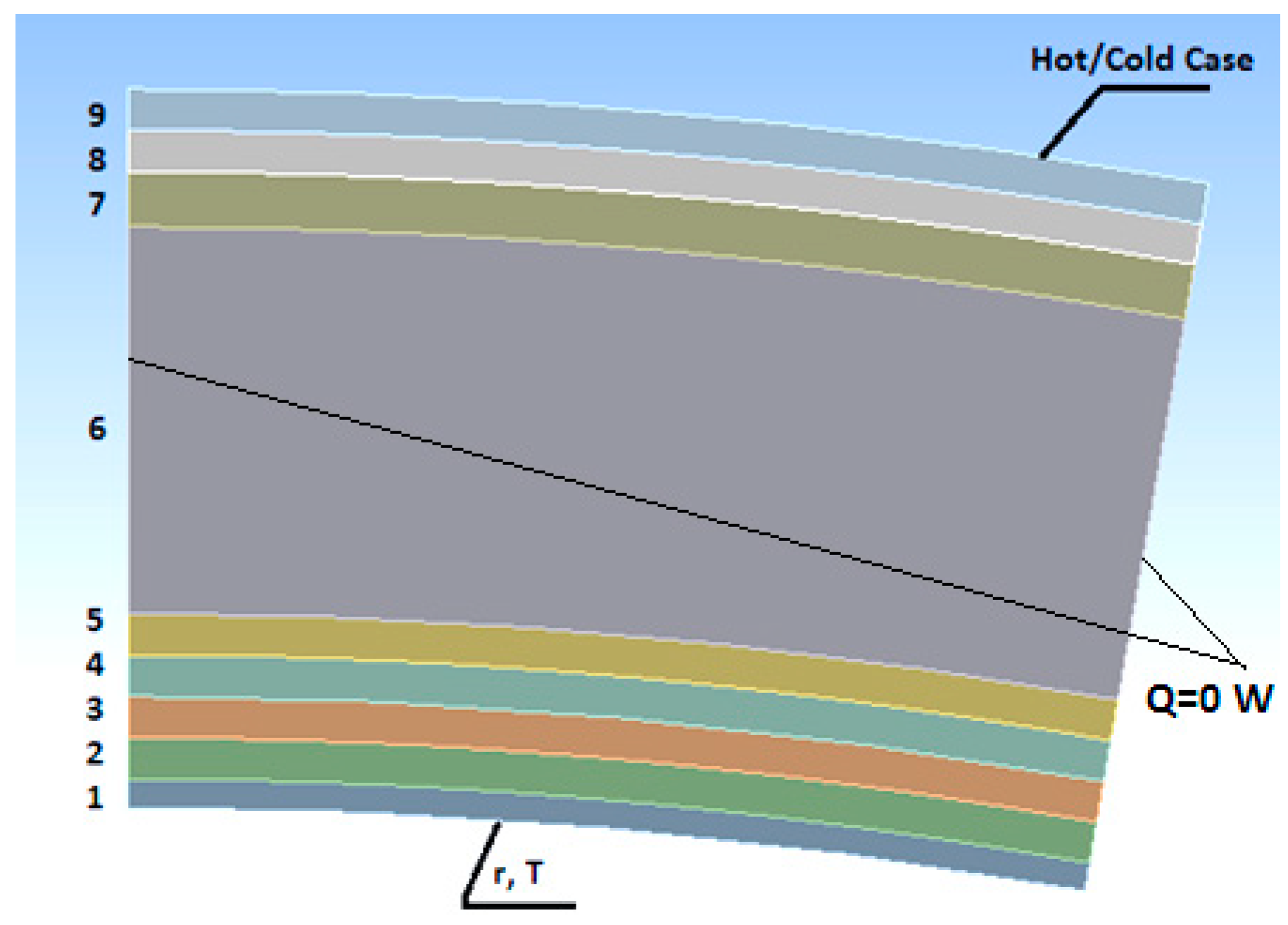
The adopted model has the shape of a multilayer cylindrical partition, with a 40 mm inner radius from the axis, which corresponds to the astronaut’s forearm. The remaining parts of the suit may contain electrical elements and other systems, causing changes in the obtained results [
31]. In the case of a repeatable shape and thermal conditions, the typical procedure is to introduce only a part of the structure during the calculations. The human forearm implies the cylindrical shape of the garment, i.e., the axisymmetric problem. Therefore, only a part of the axisymmetric structure is introduced, which is a fragment in the form of a circular sector. In order to lessen the computational requirements in the model, only the part with an opening angle of 10° was considered. The distribution of the material layers, thickness and thermal conductivity coefficients were acquired from an available material database [
32], as shown in
Table 1. The multilayer mylar was classified as a single layer.
Two extreme cases of extravehicular activity were taken into consideration: a case with the highest susceptibility to the sun’s radiation effect (Hot Case T
a = 127 °C) and a case where the sun’s impact was the lowest (Cold Case, T
a = −156 °C). Such temperatures are described by NASA as present in the area near the Moon [
6]. The CT was set to 37 °C. Heat exchange occurs between the human body and the environment, which makes it possible to insulate the side surfaces of the model.
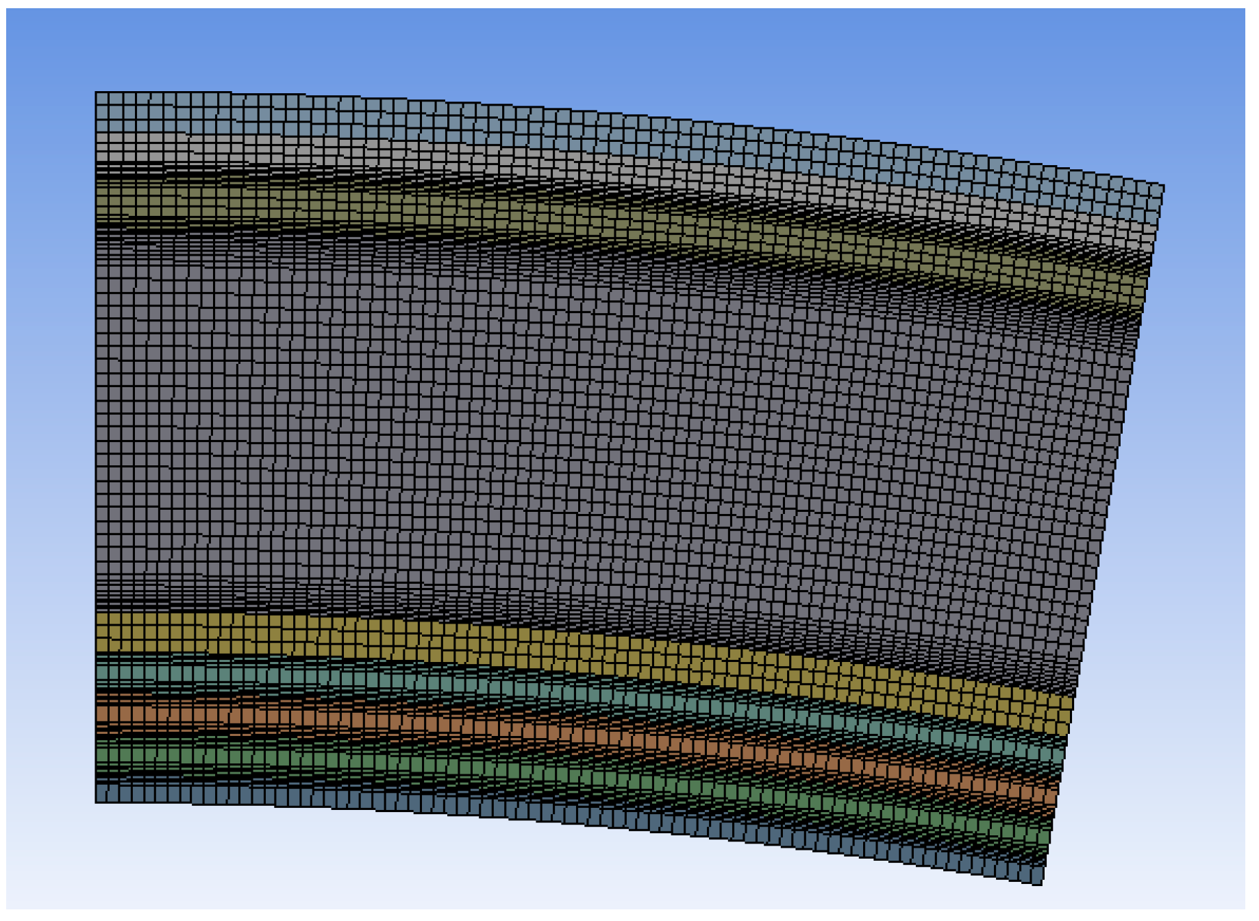
The models analyzed here are approximated with the same FEM mesh. The global size of a finite factor was chosen according to the thickness of the thinnest layer (of skin), which is equal to 0.1 mm. A decrease in size below this value would not affect the solution. The computational requirements of the model increase significantly with the number of elements. However, the changes in the accuracy of the obtained results are not visible above the determined mesh density.
A good method to improve the quality of the computational results is to increase the finite element order. Thus, the computational model requires additional nodes at the finite element boundaries, which significantly increases the number of degrees of freedom. The interpolation between the finite elements is consequently nonlinear. The disadvantage of this method is the high computational effort of nonlinear approximations compared with other solutions. The finite element order was set to 1; hence, the approximations of nodal values are described with linear equations [
33]. The increase in the finite element order did not cause a notable improvement in the results with a fixed size of the particular element [
34,
35].
Due to the model’s three-dimensional nature, the Sweep function was utilized to permit the transposition of the mesh created on one of the model’s surfaces into the third dimension. Hence, the mesh is even, preventing approximation errors and facilitating the use of other functions.
To solve a case, it is best to utilize the hexagonal elements. Nevertheless, during mesh generation, unwanted tetragonal elements may occur. The application of the MultiZone function prevents the creation of tetragonal elements.
A sudden change in the thermal conductivity coefficient takes place at the meeting point of the materials. In such areas, computational requirements are the highest due to the sudden changes in the parameters. For layers exemplifying the biggest differences in the thermal conductivity coefficient, the
Inflation function was used, which creates inflation layers with a relatively high value of the proportionality coefficient. The initial thickness of the layer at the edge was 20 μm, with each following generated layer being thicker by 10%. The number of the generated layers is between 3 and 8, depending on the changes in the conductivity coefficient on the layers’ boundaries and on their thickness (
Figure 2).
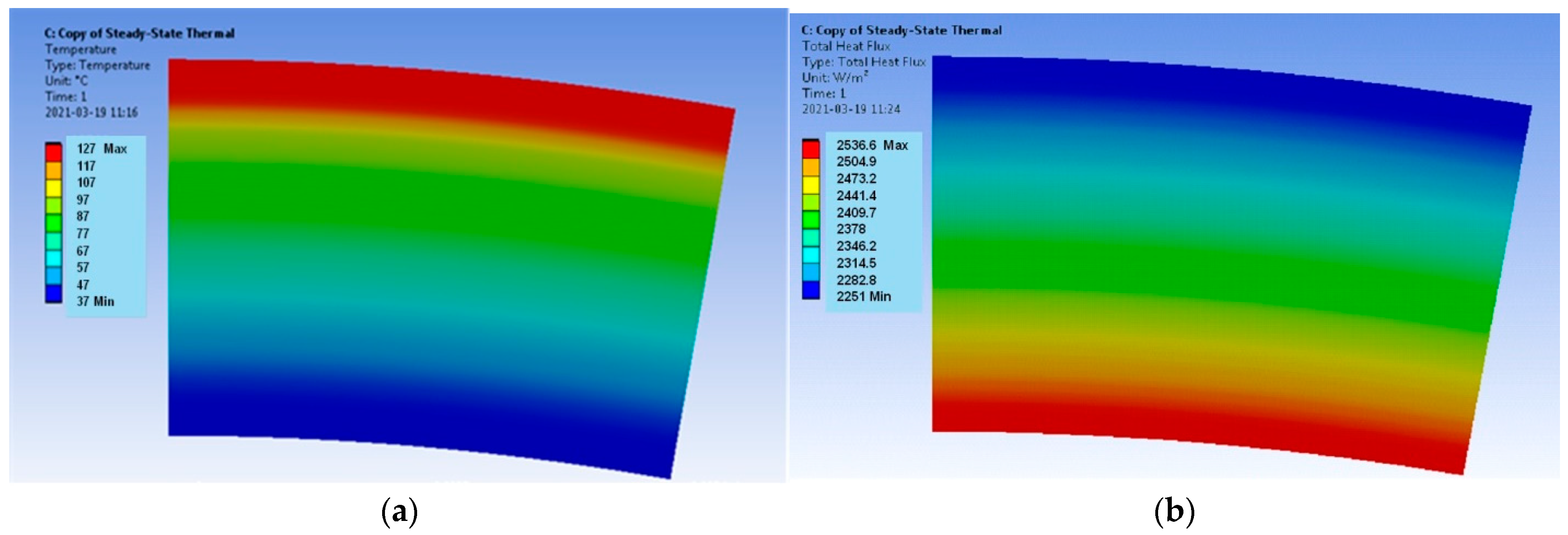
The verification model describes only the heat conduction between the layers of the material. In this way, the distribution of heat areas and the heat flux density are substantially different from the actual model, though still allowing for the assessment of the applied mesh. Only temperatures on the external surfaces of the spacesuit and the astronaut’s body are considered.
The actual model takes into account the heat radiation emission from the surface of the space suit. The suits are covered with white Krylon paint on their surface, which has an emissivity coefficient of ε = 0.98, reflecting a major part of cosmic radiation [
36]. The temperatures in the Hot and Cold Cases refer to the ambient temperature. The boundary conditions are summarized for each case in
Table 2.
2.3. Verification Calculations
The verification calculations were performed for a homogenic material of the resultant parameters. The resultant thermal conductivity coefficient is determined with the transformation of (3).
Hence, the value λ
w = 0.137125. The simplified equation describing the heat flux density on the outer layer of the suit can be defined according to (3), whereby r
0 and r are radii measured from the axis to the inner and outer layers of the space suit.
As a result of the calculations, the following values were obtained: Hot Case, T9 = 400.15 K: q = −2234.02 W/m2. Cold Case, T9 = 117.15 K; q = 4790.74 W/m2.
Using Equations (3) and (7), the temperature was determined for any contact surface.
Because radiation is the only form of heat exchange in outer space, the equation of state on the outer layer of the space suit has a following formula:
The outer layer emissivity is equal to ε = 0.98, and the reference emissivity was set to one, similar to that for a black body [
24,
36]. Therefore, the equivalent emissivity coefficient equal to ε = 0.98 was obtained.
To determine the surface temperature of the suit, Equation (9) was transformed to a fourth-degree polynomial
Hence, obtaining polynomial Equation (11) for the Cold Case and (12) for the Hot Case.
By solving the equations, the following temperatures were determined: T9,C = 301.02, K = 27.87 °C; T9,H = 326.01, K = 52.86 °C.
The density of the heat flux at any point of the model may be determined with the knowledge that the heat flux has a constant value at all points [
37]. Thus, after calculating the heat flux density on the outer layer of the space suit, the following equation was established:
The heat flux density is hence proportional to the magnitude of the instantaneous radius r
x.


