

Nanoparticle Metrology of Silicates Using Time-Resolved Multiplexed Dye Fluorescence Anisotropy, Small Angle X-ray Scattering, and Molecular Dynamics Simulations

 , , , and
Abstract
:1. Introduction
2. Materials and Methods
3. Results and Discussion
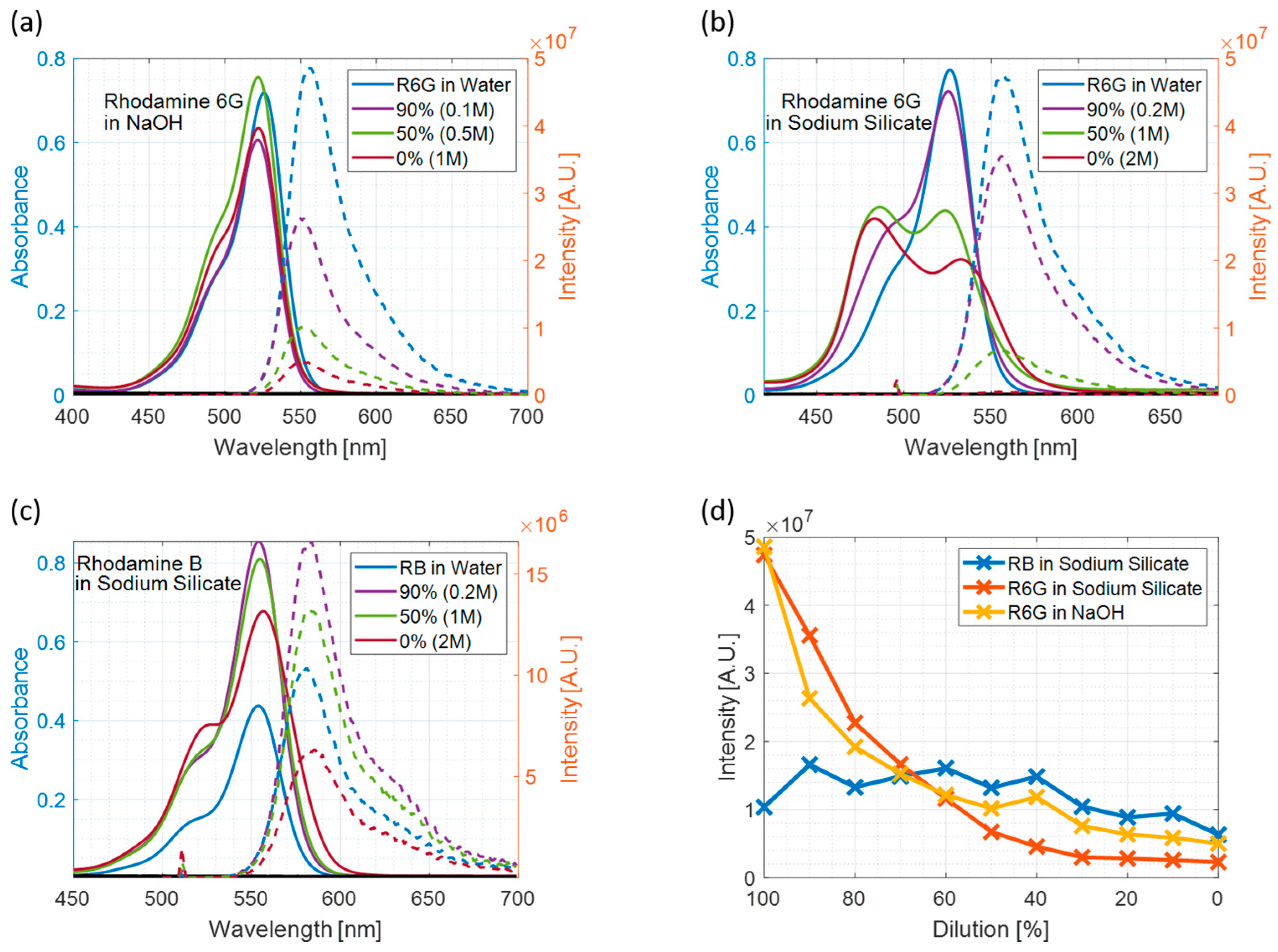
3.1. Steady-State Measurements
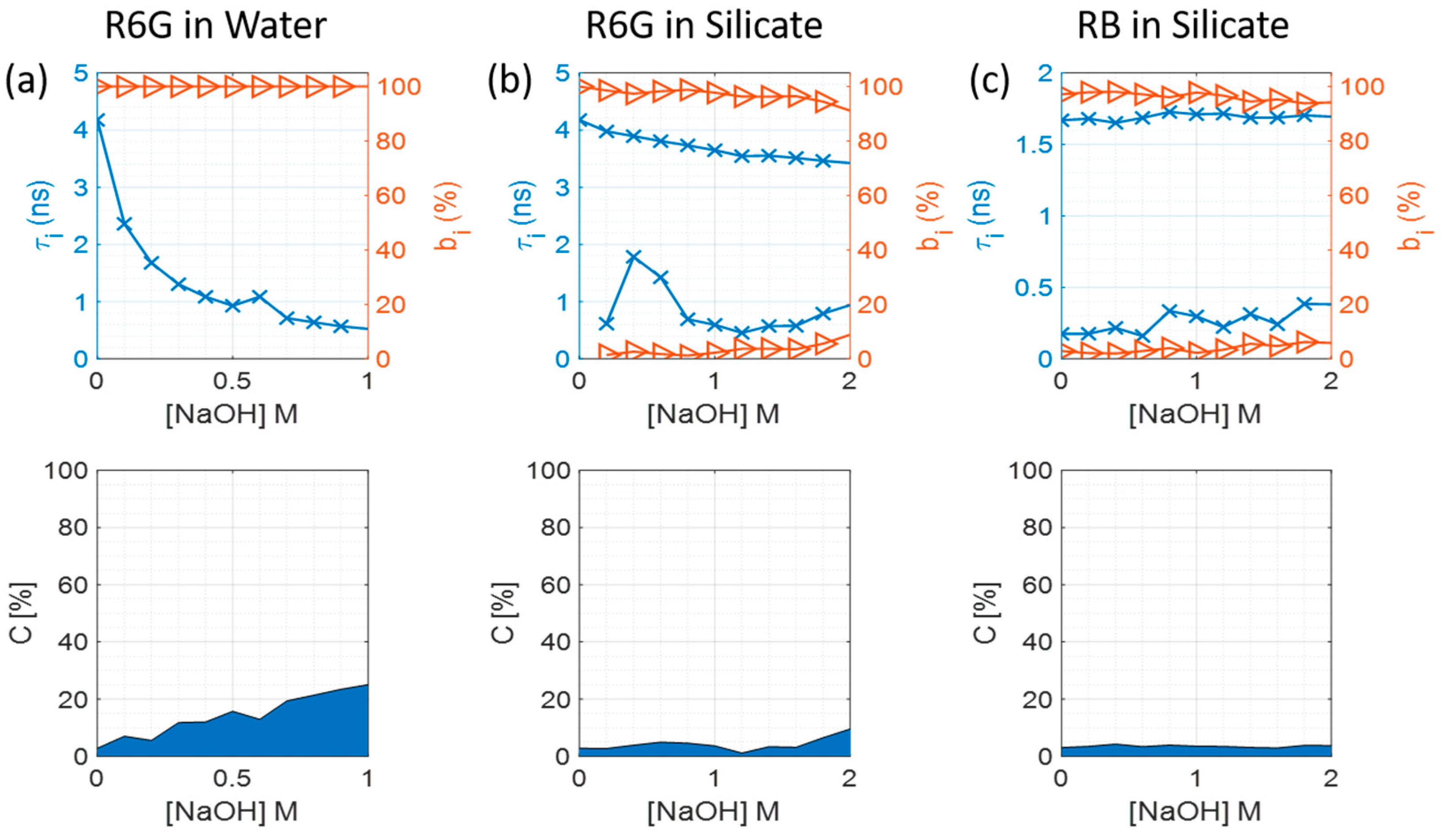
3.2. Fluorescence Decays
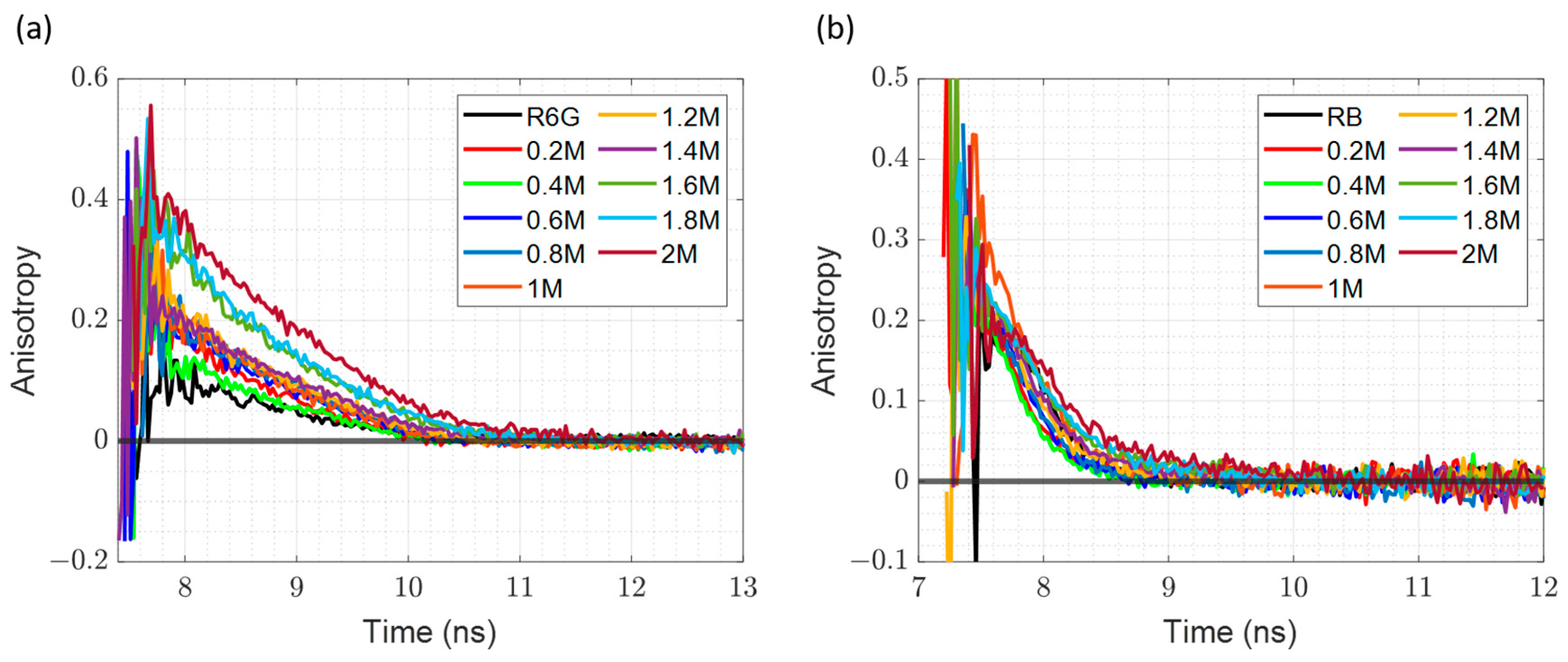
3.3. Time-Resolved Fluorescence Anisotropy in Diluted Samples
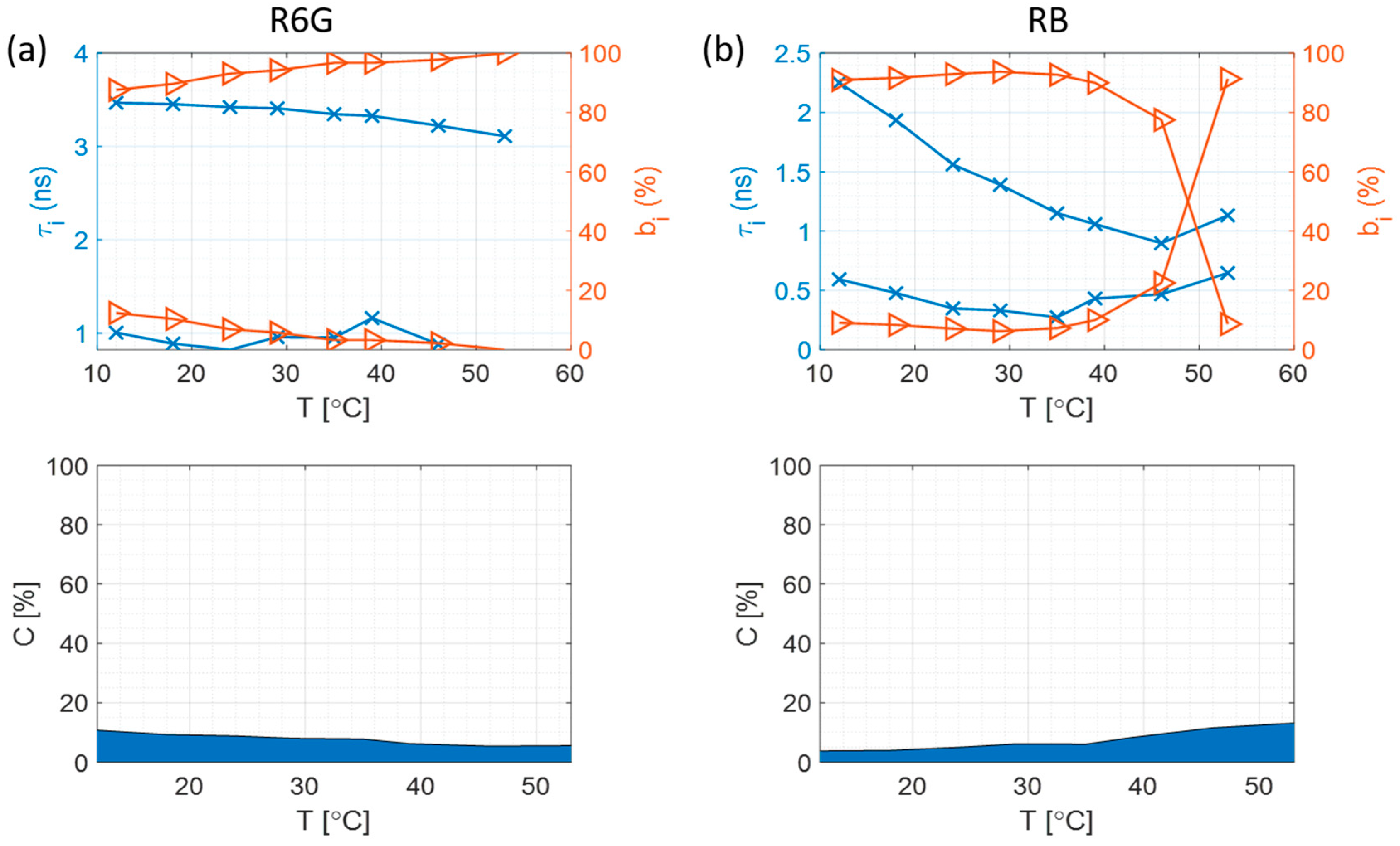
3.4. Fluorescence Intensity Decays at Different Temperatures
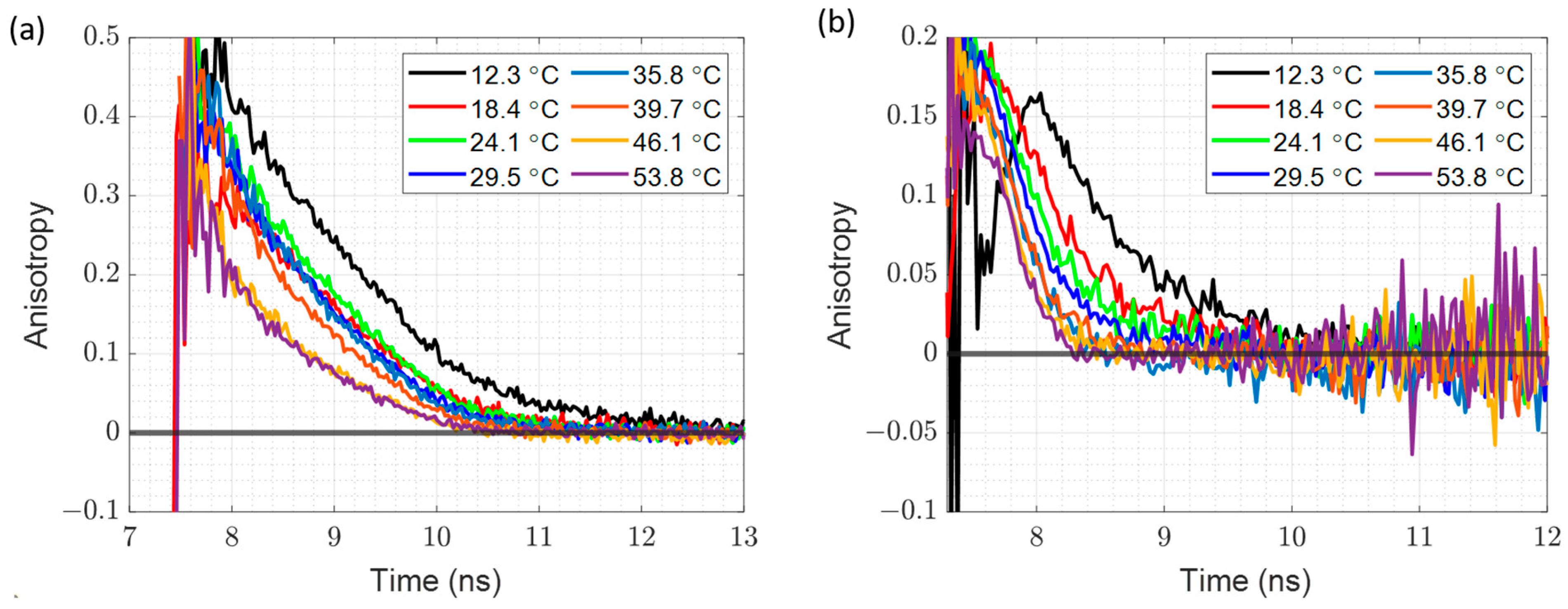
3.5. Time Resolved Fluorescence Anisotropy at Different Temperatures
3.6. Multiplexed Time-Resolved Measurements
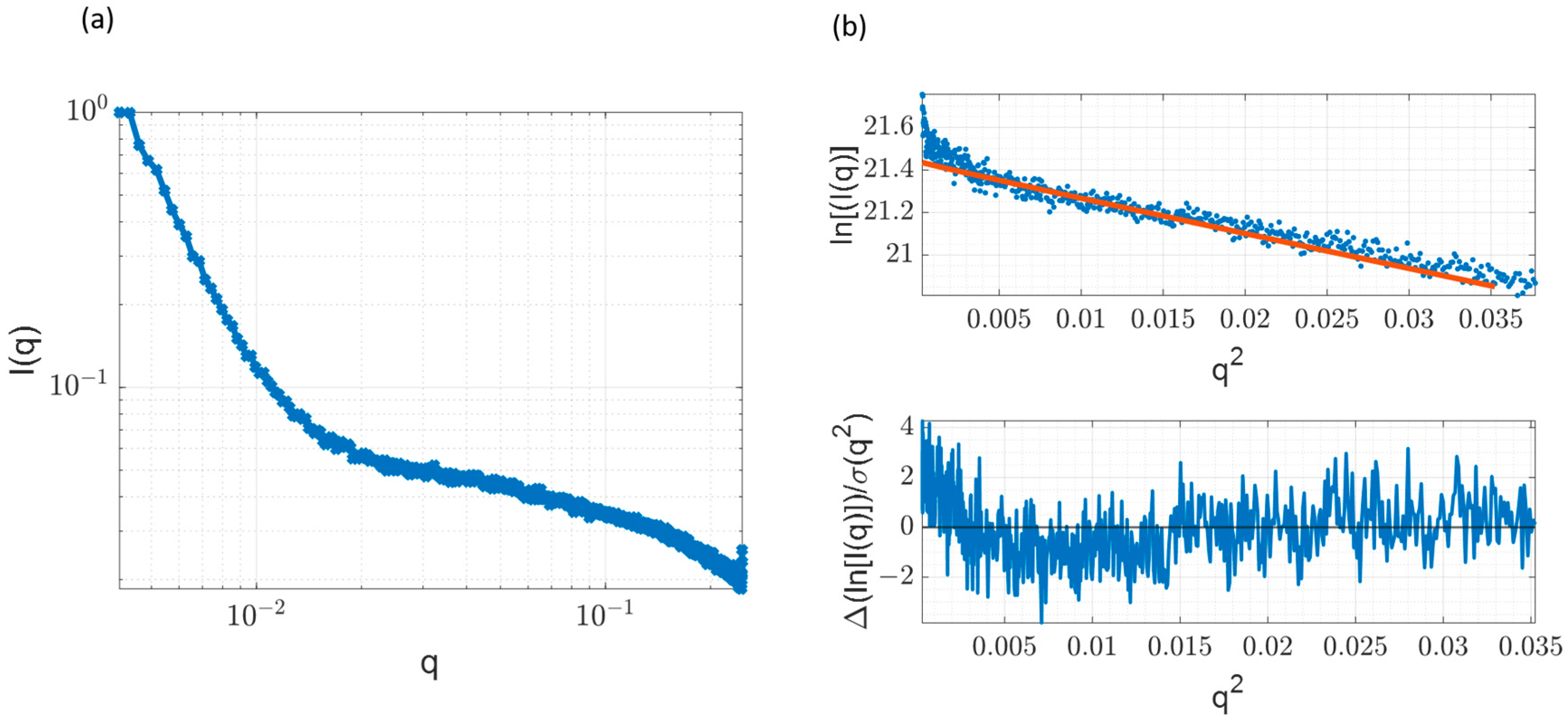
3.7. Small Angle X-ray Scattering and Comparison with Time-Resolved Anisotropy Measurements
3.8. R6G Adsorption to Silica Nanoparticles
4. Conclusions
Supplementary Materials
Author Contributions
Funding
Institutional Review Board Statement
Informed Consent Statement
Data Availability Statement
Acknowledgments
Conflicts of Interest
References
- Yang, X.; Zhu, W.; Yang, Q. The viscosity properties of sodium silicate solutions. J. Solut. Chem. 2008, 37, 73–83. [Google Scholar] [CrossRef]
- Matinfar, M.; Nychka, J.A. A review of sodium silicate solutions: Structure, gelation, and syneresis. Adv. Colloid Interface Sci. 2023, 322, 103036. [Google Scholar] [CrossRef] [PubMed]
- Stebbins, J.F. Identification of multiple structural species in silicate glasses by 29Si NMR. Nature 1987, 330, 465–467. [Google Scholar] [CrossRef] [PubMed]
- Nordström, J.; Sundblom, A.; Jensen, G.V.; Pedersen, J.S.; Palmqvist, A.; Matic, A. Silica/alkali ratio dependence of the microscopic structure of sodium silicate solutions. J. Colloid Interface Sci. 2013, 397, 9–17. [Google Scholar] [CrossRef]
- Nordström, J.; Nilsson, E.; Jarvol, P.; Nayeri, M.; Palmqvist, A.; Bergenholtz, J.; Matic, A. Concentration-and pH-dependence of highly alkaline sodium silicate solutions. J. Colloid Interface Sci. 2011, 356, 37–45. [Google Scholar] [CrossRef] [PubMed]
- Hu, G.; Jin, S.; Liu, K. Structure-Directing Effect on Silica Nanoparticle Growth in Sodium Silicate Solutions through Small-Angle X-ray Scattering. J. Phys. Chem. C 2023, 127, 10585–10593. [Google Scholar] [CrossRef]
- Uskoković, V. Dynamic light scattering based microelectrophoresis: Main prospects and limitations. J. Dispers. Sci. Technol. 2012, 33, 1762–1786. [Google Scholar] [CrossRef] [PubMed]
- Pauw, B.R. Everything SAXS: Small-angle scattering pattern collection and correction. J. Phys. Condens. Matter 2013, 25, 383201. [Google Scholar] [CrossRef] [PubMed]
- López-Lorente, Á.I.; Valcárcel, M. Chapter 1—Analytical Nanoscience and Nanotechnology. In Comprehensive Analytical Chemistry; Valcárcel, M., López-Lorente, Á.I., Eds.; Elsevier: Amsterdam, The Netherlands, 2014; Volume 66, pp. 3–35. [Google Scholar]
- Birch, D.J.; Geddes, C.D. Sol-gel particle growth studied using fluorescence anisotropy: An alternative to scattering techniques. Phys. Rev. E 2000, 62, 2977. [Google Scholar] [CrossRef]
- Yip, P.; Karolin, J.; Birch, D.J. Fluorescence anisotropy metrology of electrostatically and covalently labelled silica nanoparticles. Meas. Sci. Technol. 2012, 23, 084003. [Google Scholar] [CrossRef]
- Doveiko, D.; Kubiak-Ossowska, K.; Chen, Y. Impact of the Crystal Structure of Silica Nanoparticles on Rhodamine 6G Adsorption: A Molecular Dynamics Study. ACS Omega 2024, 9, 4123–4136. [Google Scholar] [CrossRef] [PubMed]
- Birch, D.J.; Yip, P. Nanometrology. In Fluorescence Spectroscopy and Microscopy; Springer: Berlin/Heidelberg, Germany, 2014; pp. 279–302. [Google Scholar]
- Tleugabulova, D.; Zhang, Z.; Brennan, J.D. Evolution of sodium silicate sols through the sol-to-gel transition assessed by the fluorescence-based nanoparticle metrology approach. J. Phys. Chem. B 2003, 107, 10127–10133. [Google Scholar] [CrossRef]
- Geddes, C.; Birch, D. Nanometre resolution of silica hydrogel formation using time-resolved fluorescence anisotropy. J. Non-Cryst. Solids 2000, 270, 191–204. [Google Scholar] [CrossRef]
- Szota, M.; Wolski, P.; Carucci, C.; Marincola, F.C.; Gurgul, J.; Panczyk, T.; Salis, A.; Jachimska, B. Effect of Ionization Degree of Poly(amidoamine) Dendrimer and 5-Fluorouracil on the Efficiency of Complex Formation—A Theoretical and Experimental Approach. Int. J. Mol. Sci. 2023, 24, 819. [Google Scholar] [CrossRef]
- Burgert, D.R. Specification 1.05621.0000 Sodium Silicate Solution Extra Pure; EMD Millipore Corporation—A Subsidiary of Merck KgaA: Darmstadt, Germany, 2016. [Google Scholar]
- Birch, D.J.; Imhof, R.E. Time-domain fluorescence spectroscopy using time-correlated single-photon counting. Topics in Fluorescence Spectroscopy, Springer: Berlin/Heidelberg, Germany, 2002; 1–95. [Google Scholar]
- O’Connor, D.; Phillips, D. Time-Correlated Single Photon Counting; Academic Press: New York, NY, USA, 1984. [Google Scholar]
- McGuinness, C.; Sagoo, K.; McLoskey, D.; Birch, D. A new sub-nanosecond LED at 280 nm: Application to protein fluorescence. Meas. Sci. Technol. 2004, 15, L19. [Google Scholar] [CrossRef]
- O’Hagan, W.; McKenna, M.; Sherrington, D.; Rolinski, O.; Birch, D. MHz LED source for nanosecond fluorescence sensing. Meas. Sci. Technol. 2001, 13, 84. [Google Scholar] [CrossRef]
- Brochon, J.-C. Maximum entropy method of data analysis in time-resolved spectroscopy. In Methods in Enzymology; Elsevier: Amsterdam, The Netherlands, 1994; Volume 240, pp. 262–311. [Google Scholar]
- Bharill, S.; Sarkar, P.; Ballin, J.D.; Gryczynski, I.; Wilson, G.M.; Gryczynski, Z. Fluorescence intensity decays of 2-aminopurine solutions: Lifetime distribution approach. Anal. Biochem. 2008, 377, 141–149. [Google Scholar] [CrossRef] [PubMed]
- Bajzer, Ž.; Therneau, T.M.; Sharp, J.C.; Prendergast, F.G. Maximum likelihood method for the analysis of time-resolved fluorescence decay curves. Eur. Biophys. J. 1991, 20, 247–262. [Google Scholar] [CrossRef]
- Li, Y.; Natakorn, S.; Chen, Y.; Safar, M.; Cunningham, M.; Tian, J.; Li, D.D.-U. Investigations on average fluorescence lifetimes for visualizing multi-exponential decays. Front. Phys. 2020, 8, 576862. [Google Scholar] [CrossRef]
- Luchowski, R.; Gryczynski, Z.; Sarkar, P.; Borejdo, J.; Szabelski, M.; Kapusta, P.; Gryczynski, I. Instrument response standard in time-resolved fluorescence. Rev. Sci. Instrum. 2009, 80, 033109. [Google Scholar] [CrossRef]
- Lakowicz, J.R.; Shen, B.; Gryczynski, Z.; D’Auria, S.; Gryczynski, I. Intrinsic Fluorescence from DNA Can Be Enhanced by Metallic Particles. Biochem. Biophys. Res. Commun. 2001, 286, 875–879. [Google Scholar] [CrossRef] [PubMed]
- Selanger, K.; Falnes, J.; Sikkeland, T. Fluorescence lifetime studies of Rhodamine 6G in methanol. J. Phys. Chem. 1977, 81, 1960–1963. [Google Scholar] [CrossRef]
- Stryer, L. Fluorescence Spectroscopy of Proteins: Fluorescent probes provide insight into the structure, interactions, and dynamics of proteins. Science 1968, 162, 526–533. [Google Scholar] [CrossRef] [PubMed]
- Alghamdi, A.; Vyshemirsky, V.; Birch, D.J.; Rolinski, O.J. Detecting beta-amyloid aggregation from time-resolved emission spectra. Methods Appl. Fluoresc. 2018, 6, 024002. [Google Scholar] [CrossRef]
- Rolinski, O.J.; McLaughlin, D.; Birch, D.J.; Vyshemirsky, V. Resolving environmental microheterogeneity and dielectric relaxation in fluorescence kinetics of protein. Methods Appl. Fluoresc. 2016, 4, 024001. [Google Scholar] [CrossRef] [PubMed]
- Visser, A.; Rolinski, O.J. Basic photophysics. Am. Soc. Photobiol. 2010. Available online: http://www.photobiology.info/Visser-Rolinski.html (accessed on 1 April 2024).
- Pilz, I.; Glatter, O.; Kratky, O. [11] Small-angle X-ray scattering. In Methods in Enzymology; Elsevier: Amsterdam, The Netherlands, 1979; Volume 61, pp. 148–249. [Google Scholar]
- Hopkins, J.B.; Gillilan, R.E.; Skou, S. BioXTAS RAW: Improvements to a free open-source program for small-angle X-ray scattering data reduction and analysis. J. Appl. Crystallogr. 2017, 50, 1545–1553. [Google Scholar] [CrossRef] [PubMed]
- Neubauer, H.; Gaiko, N.; Berger, S.; Schaffer, J.; Eggeling, C.; Tuma, J.; Verdier, L.; Seidel, C.A.; Griesinger, C.; Volkmer, A. Orientational and dynamical heterogeneity of rhodamine 6G terminally attached to a DNA helix revealed by NMR and single-molecule fluorescence spectroscopy. J. Am. Chem. Soc. 2007, 129, 12746–12755. [Google Scholar] [CrossRef]
- Chuichay, P.; Vladimirov, E.; Siriwong, K.; Hannongbua, S.; Rösch, N. Molecular-dynamics simulations of pyronine 6G and rhodamine 6G dimers in aqueous solution. J. Mol. Model. 2006, 12, 885–896. [Google Scholar] [CrossRef] [PubMed]
- Jo, S.; Kim, T.; Iyer, V.G.; Im, W. CHARMM-GUI: A web-based graphical user interface for CHARMM. J. Comput. Chem. 2008, 29, 1859–1865. [Google Scholar] [CrossRef]
- Choi, Y.K.; Kern, N.R.; Kim, S.; Kanhaiya, K.; Afshar, Y.; Jeon, S.H.; Jo, S.; Brooks, B.R.; Lee, J.; Tadmor, E.B. CHARMM-GUI nanomaterial modeler for modeling and simulation of nanomaterial systems. J. Chem. Theory Comput. 2021, 18, 479–493. [Google Scholar] [CrossRef]
- Humphrey, W.; Dalke, A.; Schulten, K. VMD: Visual molecular dynamics. J. Mol. Graph. 1996, 14, 33–38. [Google Scholar] [CrossRef] [PubMed]
- Phillips, J.C.; Braun, R.; Wang, W.; Gumbart, J.; Tajkhorshid, E.; Villa, E.; Chipot, C.; Skeel, R.D.; Kale, L.; Schulten, K. Scalable molecular dynamics with NAMD. J. Comput. Chem. 2005, 26, 1781–1802. [Google Scholar] [CrossRef]
- Phillips, J.C.; Hardy, D.J.; Maia, J.D.; Stone, J.E.; Ribeiro, J.V.; Bernardi, R.C.; Buch, R.; Fiorin, G.; Hénin, J.; Jiang, W. Scalable molecular dynamics on CPU and GPU architectures with NAMD. J. Chem. Phys. 2020, 153, 044130. [Google Scholar] [CrossRef] [PubMed]
- Heinz, H.; Lin, T.-J.; Kishore Mishra, R.; Emami, F.S. Thermodynamically consistent force fields for the assembly of inorganic, organic, and biological nanostructures: The INTERFACE force field. Langmuir 2013, 29, 1754–1765. [Google Scholar] [CrossRef] [PubMed]
- Huang, J.; MacKerell, A.D., Jr. CHARMM36 all-atom additive protein force field: Validation based on comparison to NMR data. J. Comput. Chem. 2013, 34, 2135–2145. [Google Scholar] [CrossRef] [PubMed]
- Mark, P.; Nilsson, L. Structure and dynamics of the TIP3P, SPC, and SPC/E water models at 298 K. J. Phys. Chem. A 2001, 105, 9954–9960. [Google Scholar] [CrossRef]
- Malfatti, L.; Kidchob, T.; Aiello, D.; Aiello, R.; Testa, F.; Innocenzi, P. Aggregation states of rhodamine 6G in mesostructured silica films. J. Phys. Chem. C 2008, 112, 16225–16230. [Google Scholar] [CrossRef]
- Anedda, A.; Carbonaro, C.M.; Corpino, R.; Ricci, P.C.; Grandi, S.; Mustarelli, P. Formation of fluorescent aggregates in Rhodamine 6G doped silica glasses. J. Non-Cryst. Solids 2007, 353, 481–485. [Google Scholar] [CrossRef]
- Haimerl, J.M.; Ghosh, I.; König, B.; Lupton, J.M.; Vogelsang, J. Chemical photocatalysis with rhodamine 6g: Investigation of photoreduction by simultaneous fluorescence correlation spectroscopy and fluorescence lifetime measurements. J. Phys. Chem. B 2018, 122, 10728–10735. [Google Scholar] [CrossRef]
- Müller, C.; Loman, A.; Pacheco, V.; Koberling, F.; Willbold, D.; Richtering, W.; Enderlein, J. Precise measurement of diffusion by multi-color dual-focus fluorescence correlation spectroscopy. Europhys. Lett. 2008, 83, 46001. [Google Scholar] [CrossRef]
- Gumy, J.-C.; Vauthey, E. Picosecond polarization grating study of the effect of excess excitation energy on the rotational dynamics of rhodamine 6G in different electronic states. J. Phys. Chem. 1996, 100, 8628–8632. [Google Scholar] [CrossRef]
- D’Arrigo, J.S. Screening of membrane surface charges by divalent cations: An atomic representation. Am. J. Physiol.-Cell Physiol. 1978, 235, C109–C117. [Google Scholar] [CrossRef] [PubMed]
- Trease, N.M.; Clark, T.M.; Grandinetti, P.J.; Stebbins, J.F.; Sen, S. Bond length-bond angle correlation in densified silica—Results from 17O NMR spectroscopy. J. Chem. Phys. 2017, 146, 184505. [Google Scholar] [CrossRef]
- Lakowicz, J. Principles of Fluorescence Spectroscopy; Springer: Boston, MA, USA, 2006. [Google Scholar]
- Aguilar-Caballos, M.P.; Gómez-Hens, A.; Pérez-Bendito, D. Simultaneous stopped-flow determination of butylated hydroxyanisole and propyl gallate using a T-format luminescence spectrometer. J. Agric. Food Chem. 2000, 48, 312–317. [Google Scholar] [CrossRef] [PubMed]
- Birch, D.; Holmes, A.; Gilchrist, J.; Imhof, R.; Al Alawi, S.; Nadolski, B. A multiplexed single-photon instrument for routine measurement of time-resolved fluorescence anisotropy. J. Phys. E Sci. Instrum. 1987, 20, 471. [Google Scholar] [CrossRef]
- Sutherland, J.C. Simultaneous measurement of circular dichroism and fluorescence polarization anisotropy. In Proceedings of the Clinical Diagnostic Systems: Technologies and Instrumentation, San Jose, CA, USA, 22–24 January 2002; pp. 126–136. [Google Scholar]
- Kufcsák, A.; Erdogan, A.; Walker, R.; Ehrlich, K.; Tanner, M.; Megia-Fernandez, A.; Scholefield, E.; Emanuel, P.; Dhaliwal, K.; Bradley, M. Time-resolved spectroscopy at 19,000 lines per second using a CMOS SPAD line array enables advanced biophotonics applications. Opt. Express 2017, 25, 11103–11123. [Google Scholar] [CrossRef] [PubMed]
- Tande, B.M.; Wagner, N.J.; Mackay, M.E.; Hawker, C.J.; Jeong, M. Viscosimetric, hydrodynamic, and conformational properties of dendrimers and dendrons. Macromolecules 2001, 34, 8580–8585. [Google Scholar] [CrossRef]
- Eichler, H.; Klein, U.; Langhans, D. Measurement of orientational relaxation times of rhodamine 6G with a streak camera. Chem. Phys. Lett. 1979, 67, 21–23. [Google Scholar] [CrossRef]


| SiO2 (%) (Estimated) | [NaOH] M (Estimated) | Rotational Time of Non-Binding Probe (RB) (ns) | Microviscosity (mPa∙s) | Rotational Time of Binding Probe (R6G) (ns) | Silica Particle Size (Å) |
|---|---|---|---|---|---|
| 27.0 | 2.0 | 0.54 ± 0.04 | 2.47 ± 0.19 | 1.16 ± 0.03 | 7.7 ± 0.8 |
| 24.3 | 1.8 | 0.46 ± 0.03 | 1.99 ± 0.12 | 0.84 ± 0.02 | 7.4 ± 0.7 |
| 21.6 | 1.6 | 0.41 ± 0.03 | 1.92 ± 0.12 | 0.40 ± 0.01 | 5.9 ± 0.5 |
| 18.9 | 1.4 | 0.35 ± 0.02 | 1.56 ± 0.11 | 0.44 ± 0.02 | 6.5 ± 0.7 |
| 16.2 | 1.2 | 0.32 ± 0.03 | 1.42 ± 0.13 | 0.27 ± 0.01 | 5.7 ± 0.8 |
| 13.5 | 1.0 | 0.40 ± 0.03 | 1.69 ± 0.14 | 0.19 ± 0.02 | 4.8 ± 0.8 |
| 10.8 | 0.8 | 0.30 ± 0.03 | 1.15 ± 0.14 | 0.24 ± 0.01 | 5.8 ± 1.0 |
| 8.1 | 0.6 | 0.25 ± 0.03 | 1.02 ± 0.12 | 0.17 ± 0.02 | 5.4 ± 1.2 |
| 5.4 | 0.4 | 0.26 ± 0.02 | 1.04 ± 0.16 | 0.19 ± 0.003 | 5.6 ± 1.4 |
| 2.7 | 0.2 | 0.22 ± 0.04 | 1.25 ± 0.11 | 0.14 ± 0.02 | 4.7 ± 1.2 |
| T (°C) | Rotational Time of Non-Binding Probe (RB) (ns) | Microviscosity (mPa∙s) | Rotational Time of Binding Probe (R6G) (ns) | Silica Particle Size (Å) |
|---|---|---|---|---|
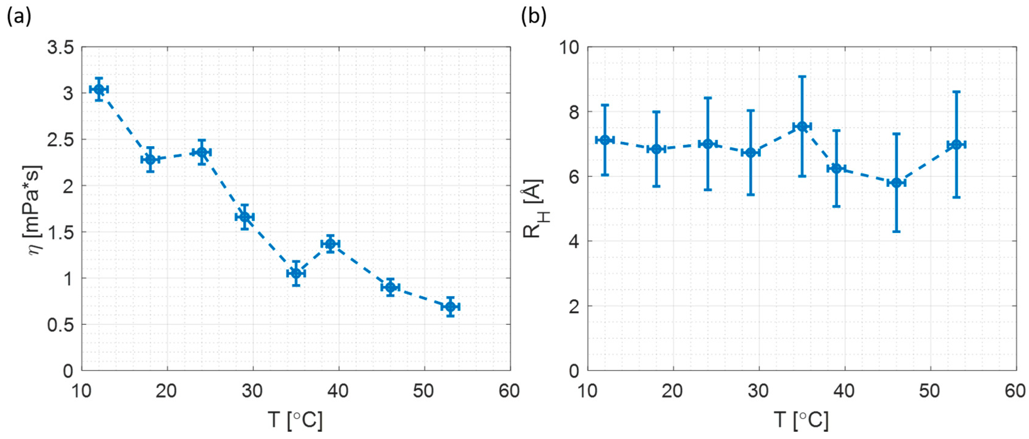
| 12 ± 1 | 0.72 ± 0.03 | 3.04 ± 0.12 | 1.17 ± 0.03 | 7.1 ± 1.1 |
| 18 ± 1 | 0.53 ± 0.03 | 2.28 ± 0.13 | 0.76 ± 0.03 | 6.8 ± 1.1 |
| 24 ± 1 | 0.54 ± 0.03 | 2.36 ± 0.13 | 0.82 ± 0.06 | 7.0 ± 1.4 |
| 29 ± 1 | 0.37 ± 0.03 | 1.66 ± 0.13 | 0.51 ± 0.03 | 6.7 ± 1.3 |
| 35 ± 1 | 0.23 ± 0.03 | 1.05 ± 0.13 | 0.44 ± 0.03 | 7.5 ± 1.5 |
| 39 ± 1 | 0.29 ± 0.02 | 1.37 ± 0.09 | 0.32 ± 0.03 | 6.2 ± 1.2 |
| 46 ± 1 | 0.19 ± 0.02 | 0.90 ± 0.09 | 0.18 ± 0.03 | 5.8 ± 1.5 |
| 53 ± 1 | 0.14 ± 0.02 | 0.69 ± 0.10 | 0.22 ± 0.03 | 7.0 ± 1.6 |
Disclaimer/Publisher’s Note: The statements, opinions and data contained in all publications are solely those of the individual author(s) and contributor(s) and not of MDPI and/or the editor(s). MDPI and/or the editor(s) disclaim responsibility for any injury to people or property resulting from any ideas, methods, instructions or products referred to in the content. |
© 2024 by the authors. Licensee MDPI, Basel, Switzerland. This article is an open access article distributed under the terms and conditions of the Creative Commons Attribution (CC BY) license (https://creativecommons.org/licenses/by/4.0/).
Share and Cite
Doveiko, D.; Martin, A.R.G.; Vyshemirsky, V.; Stebbing, S.; Kubiak-Ossowska, K.; Rolinski, O.; Birch, D.J.S.; Chen, Y. Nanoparticle Metrology of Silicates Using Time-Resolved Multiplexed Dye Fluorescence Anisotropy, Small Angle X-ray Scattering, and Molecular Dynamics Simulations. Materials 2024, 17, 1686. https://doi.org/10.3390/ma17071686
Doveiko D, Martin ARG, Vyshemirsky V, Stebbing S, Kubiak-Ossowska K, Rolinski O, Birch DJS, Chen Y. Nanoparticle Metrology of Silicates Using Time-Resolved Multiplexed Dye Fluorescence Anisotropy, Small Angle X-ray Scattering, and Molecular Dynamics Simulations. Materials. 2024; 17(7):1686. https://doi.org/10.3390/ma17071686
Chicago/Turabian StyleDoveiko, Daniel, Alan R. G. Martin, Vladislav Vyshemirsky, Simon Stebbing, Karina Kubiak-Ossowska, Olaf Rolinski, David J. S. Birch, and Yu Chen. 2024. "Nanoparticle Metrology of Silicates Using Time-Resolved Multiplexed Dye Fluorescence Anisotropy, Small Angle X-ray Scattering, and Molecular Dynamics Simulations" Materials 17, no. 7: 1686. https://doi.org/10.3390/ma17071686