
Rapid Prediction of Nonlinear Effective Properties of Complex Microstructure Lattice Materials


Highlights
- Data-driven FCA is introduced for elastoplastic effective analysis of complex lattice materials.
- Comparative investigation of configuration-dependent anisotropy evolution in lattice microstructures enabled by FCA efficiency advantages.
- The prediction of lattice materials based on voxel-grids using FCA has been investigated.
Abstract
1. Introduction
2. Methodology and Solution Framework
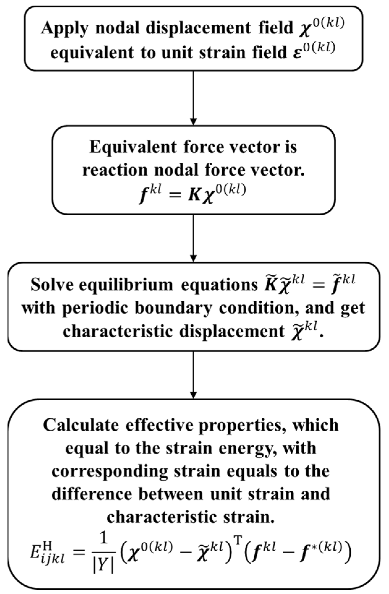
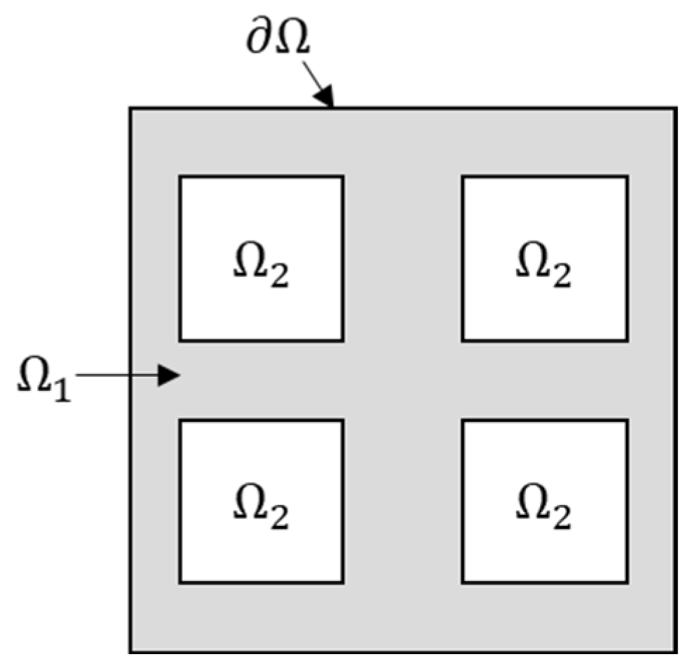
2.1. Homogenization of Lattice Materials
2.2. FCA Method for Solving the Nonlinear Effective Properties of Lattice RVEs
2.2.1. The Governing Equations of FCA
2.2.2. Offline Phase
2.2.3. Online Phase
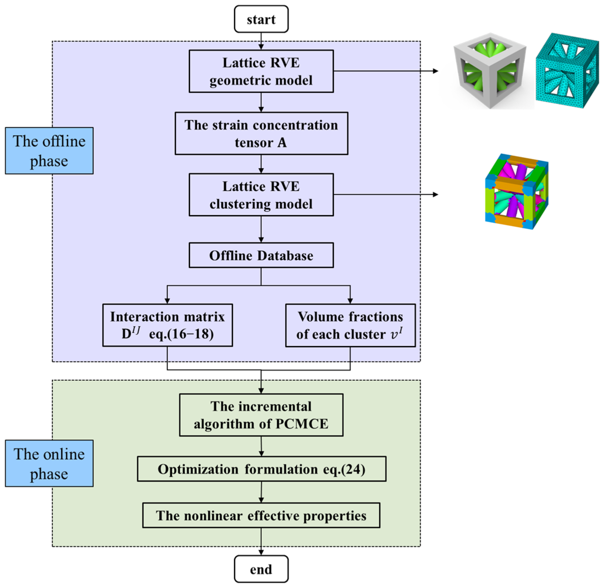
2.3. Solution Framework
3. Modeling of Complex Micro Structured Lattice Materials
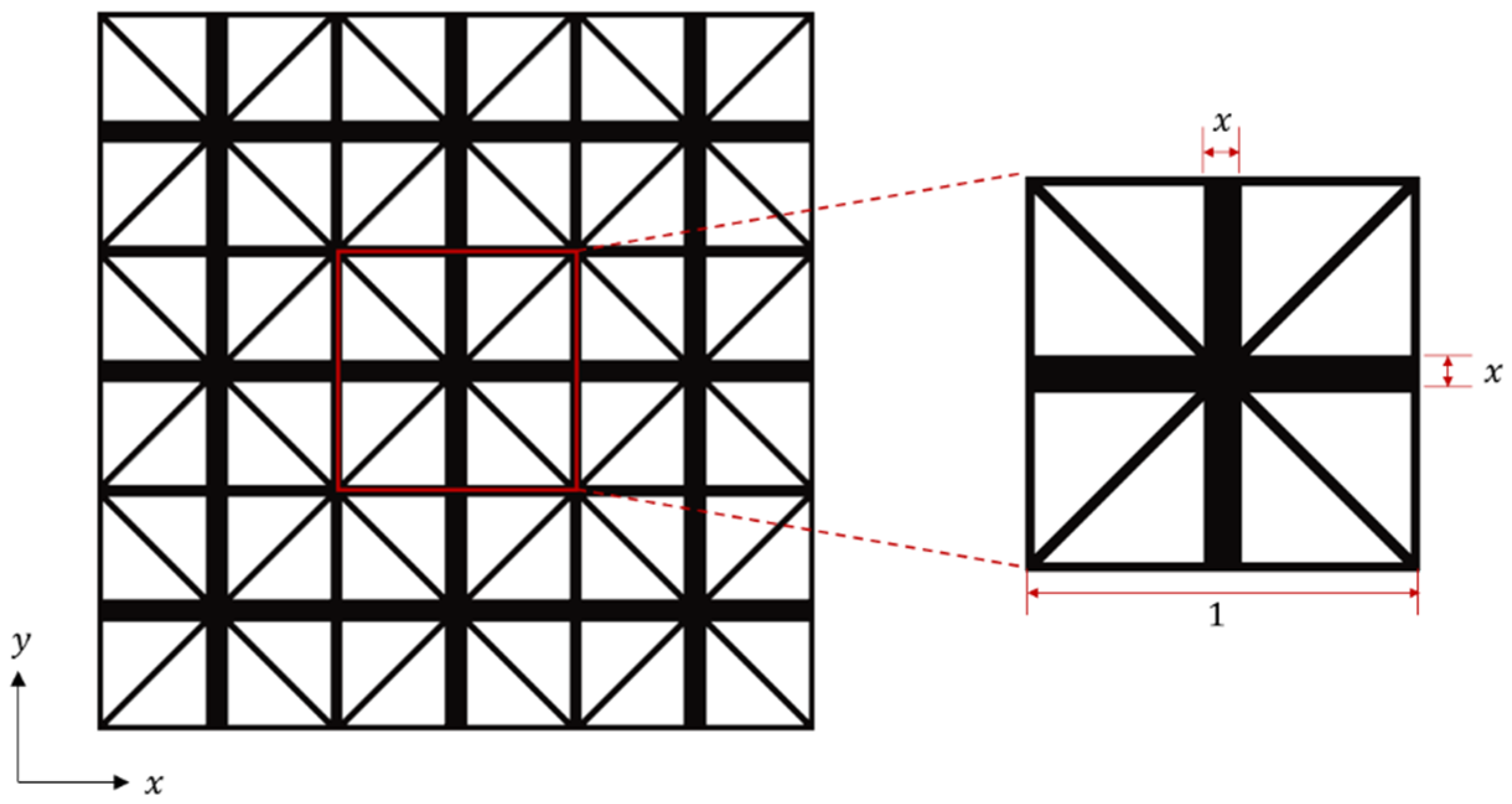
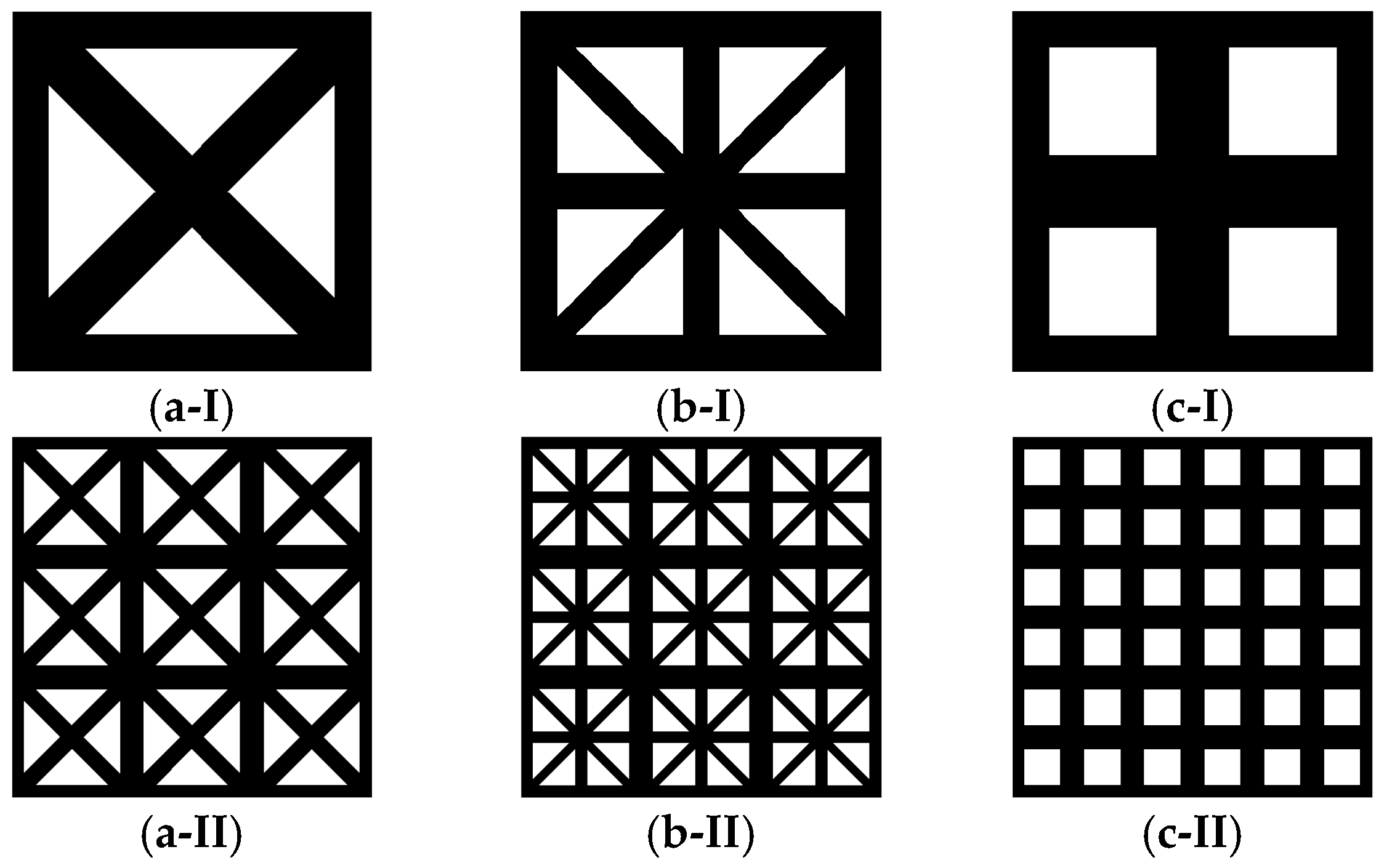
3.1. Introduction to 2D Model of Lattice Material
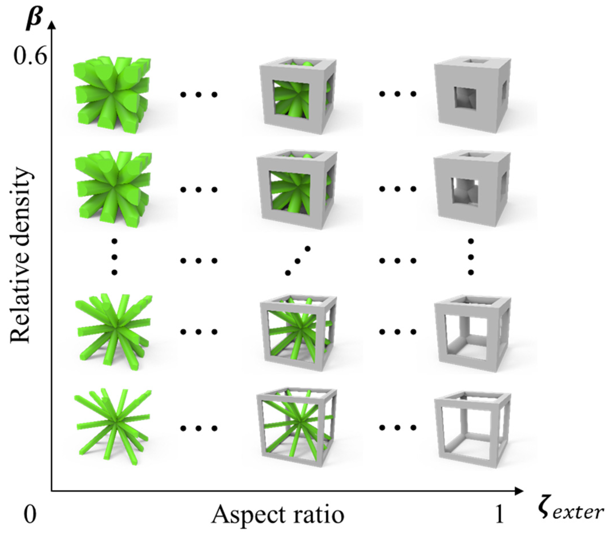
3.2. Introduction to 3D Model of Lattice Material
3.3. Introduction to Complex Voxel Lattice Modeling
3.4. Material Constitutive Parameters
4. Comparison and Discussion of Elastoplastic Effective Properties
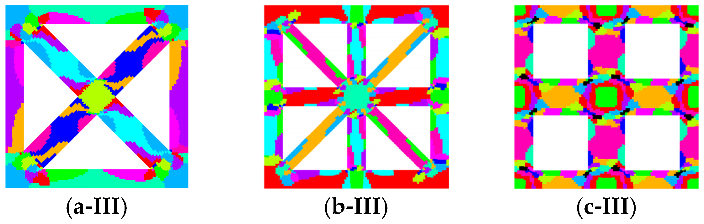
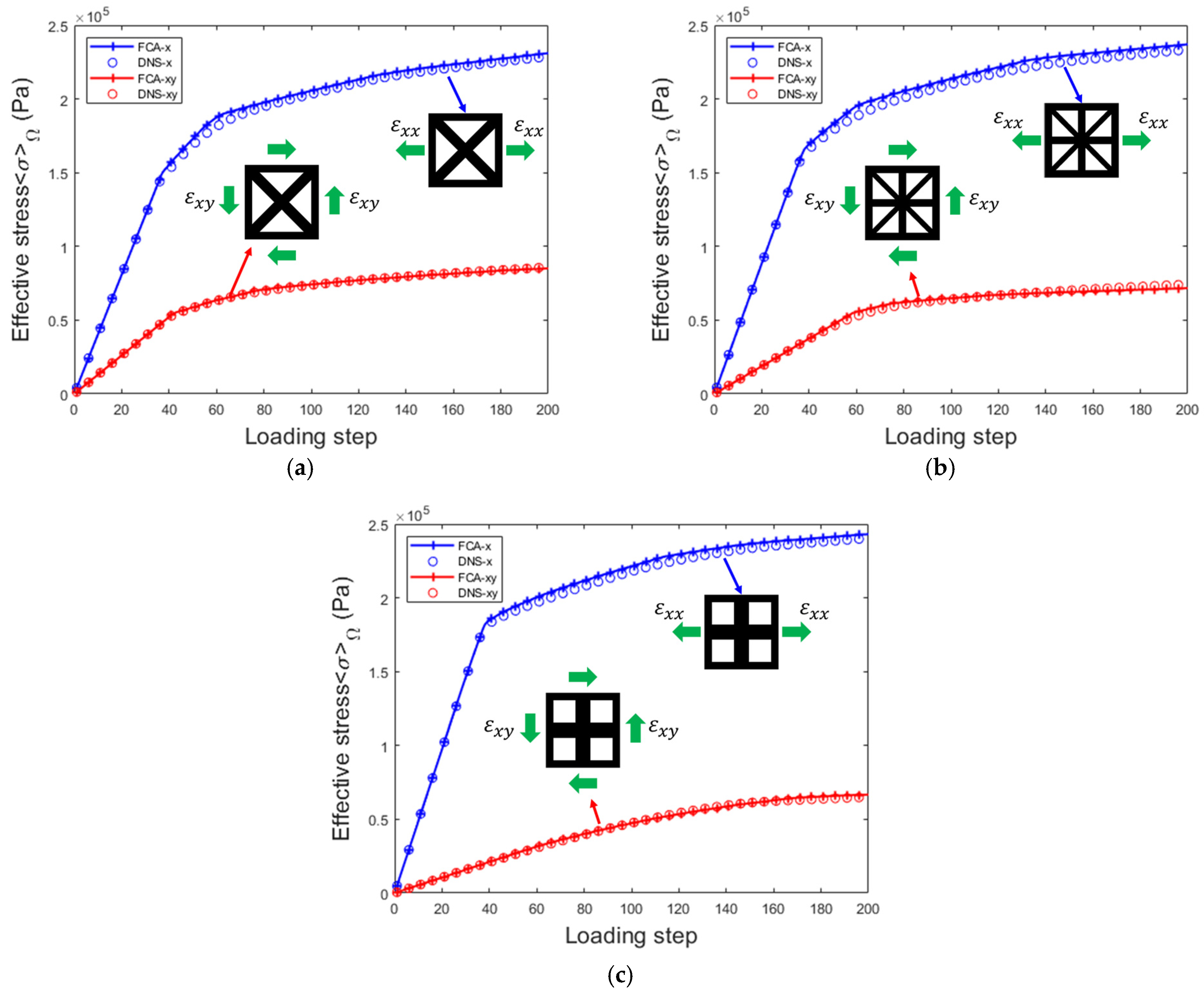
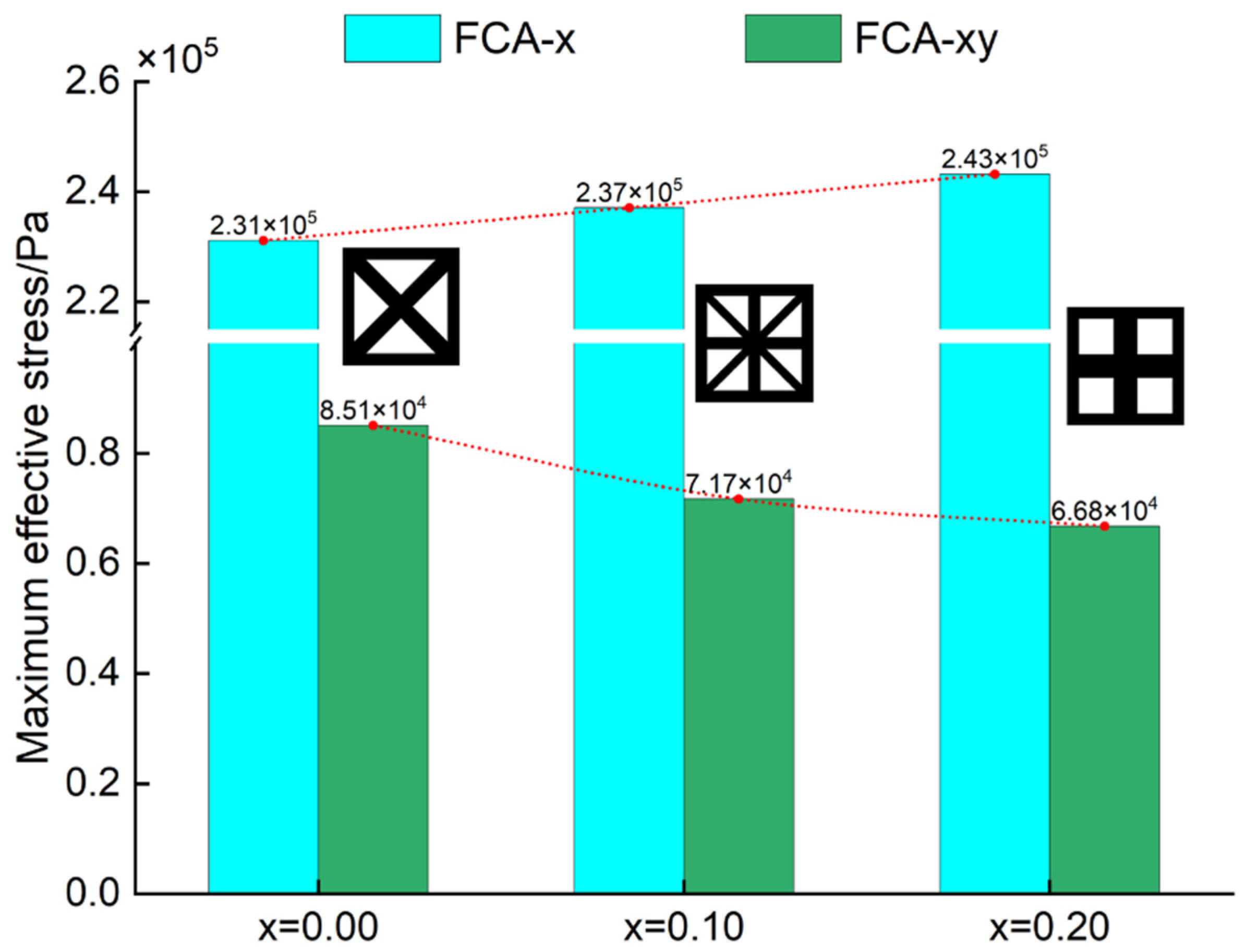
4.1. 2D Results of Effective Properties Analysis
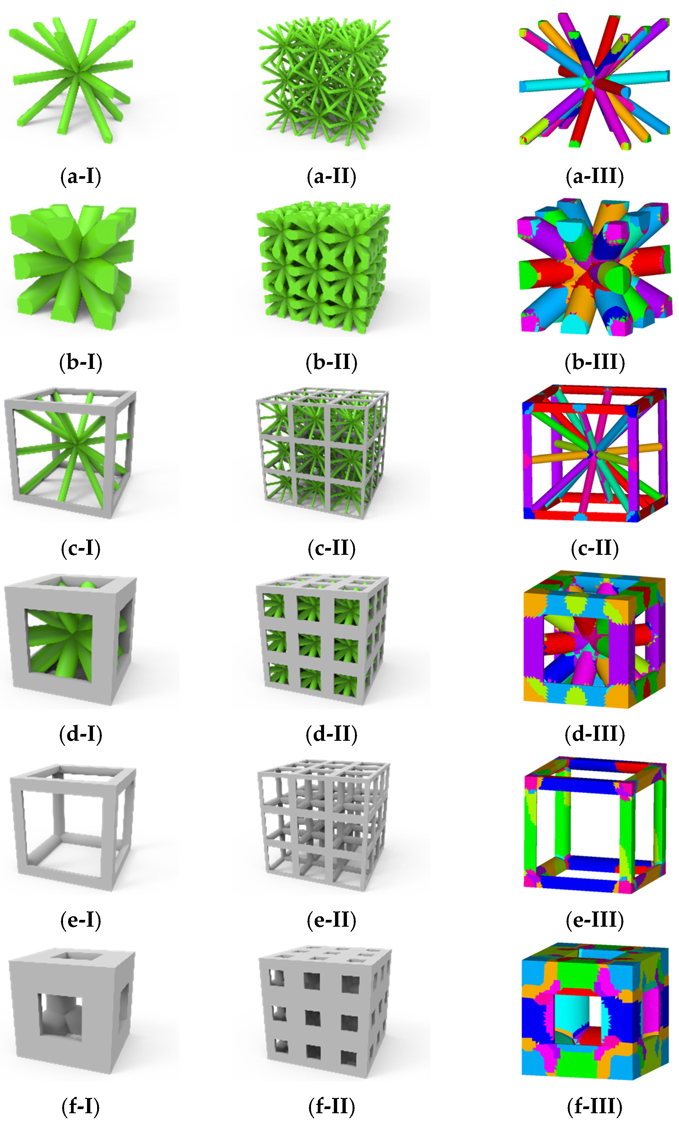
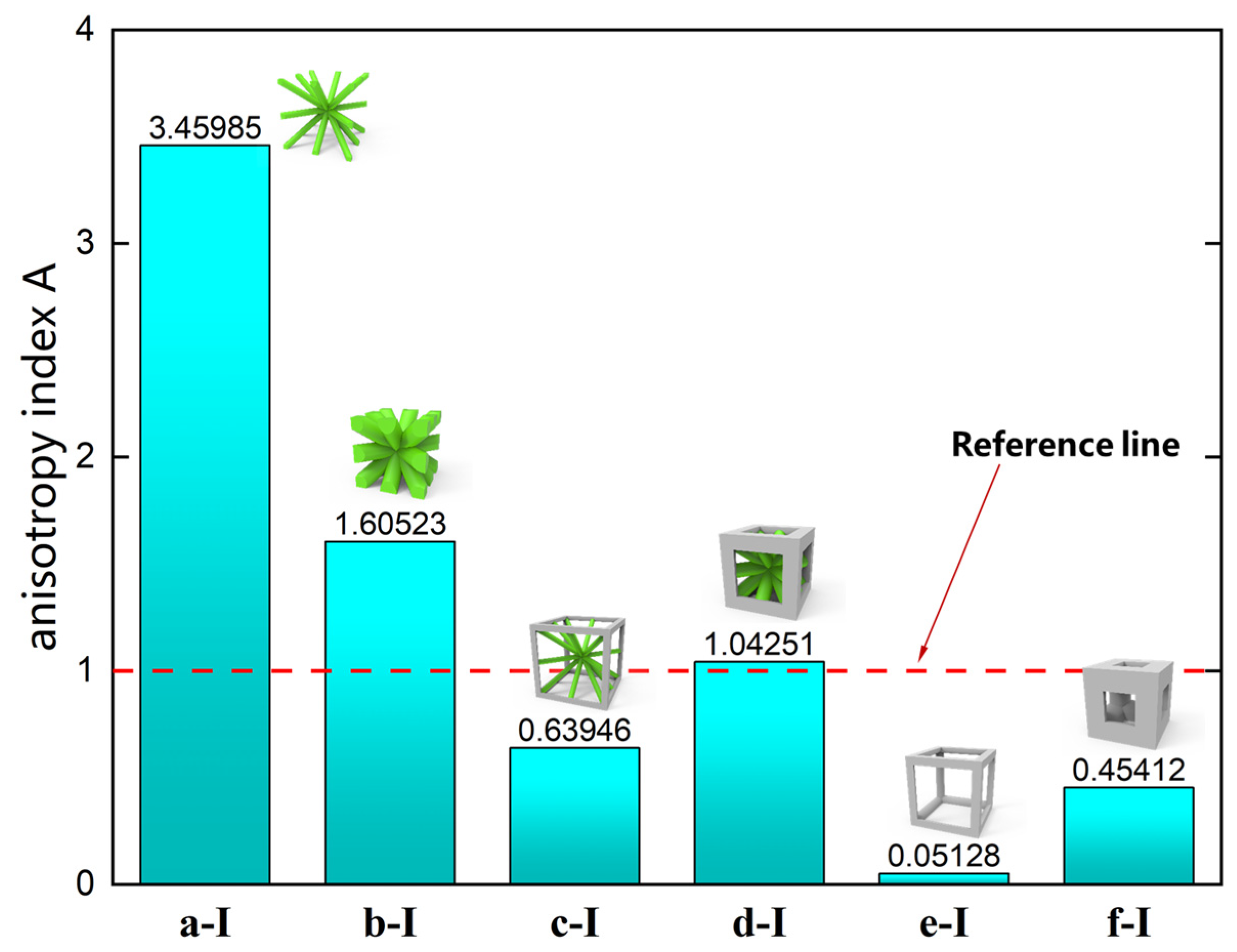
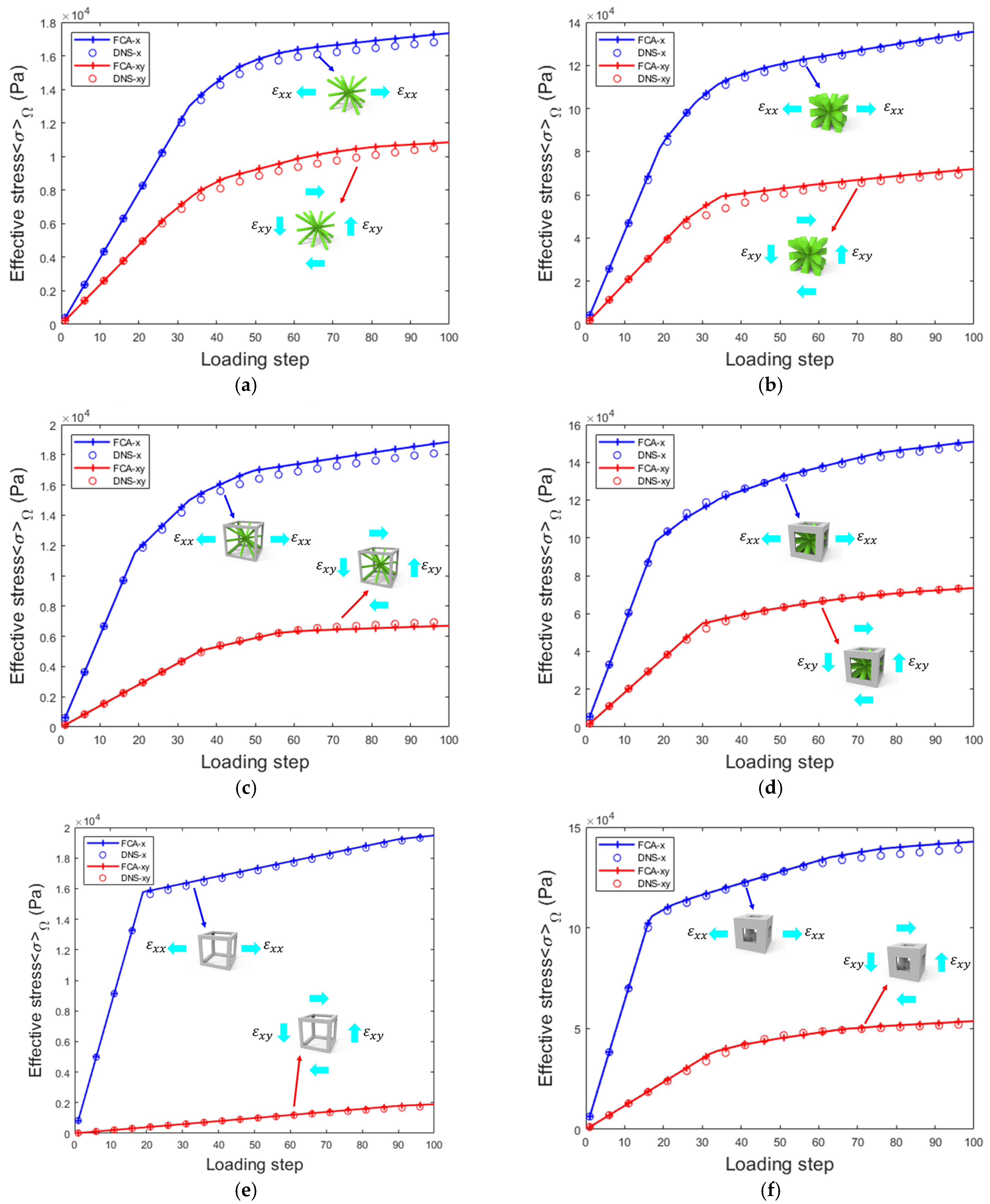
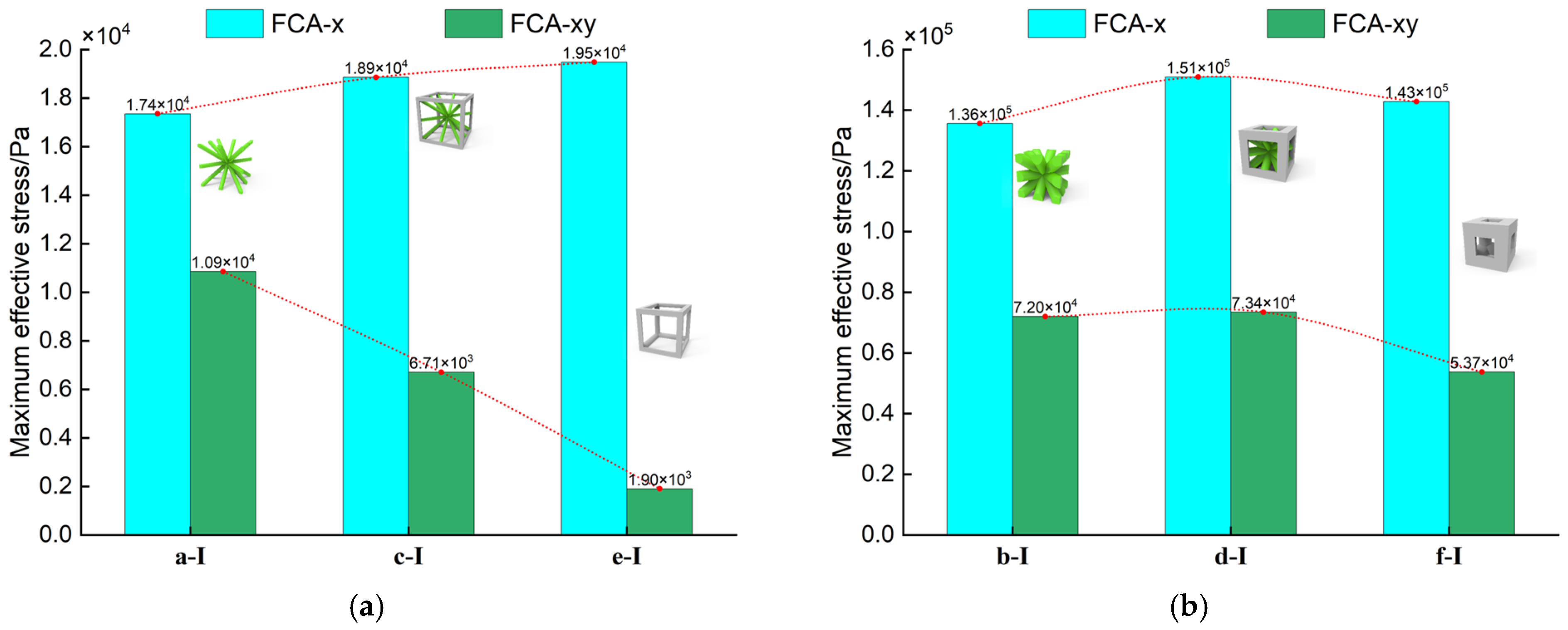
4.2. 3D Results of Effective Properties Analysis
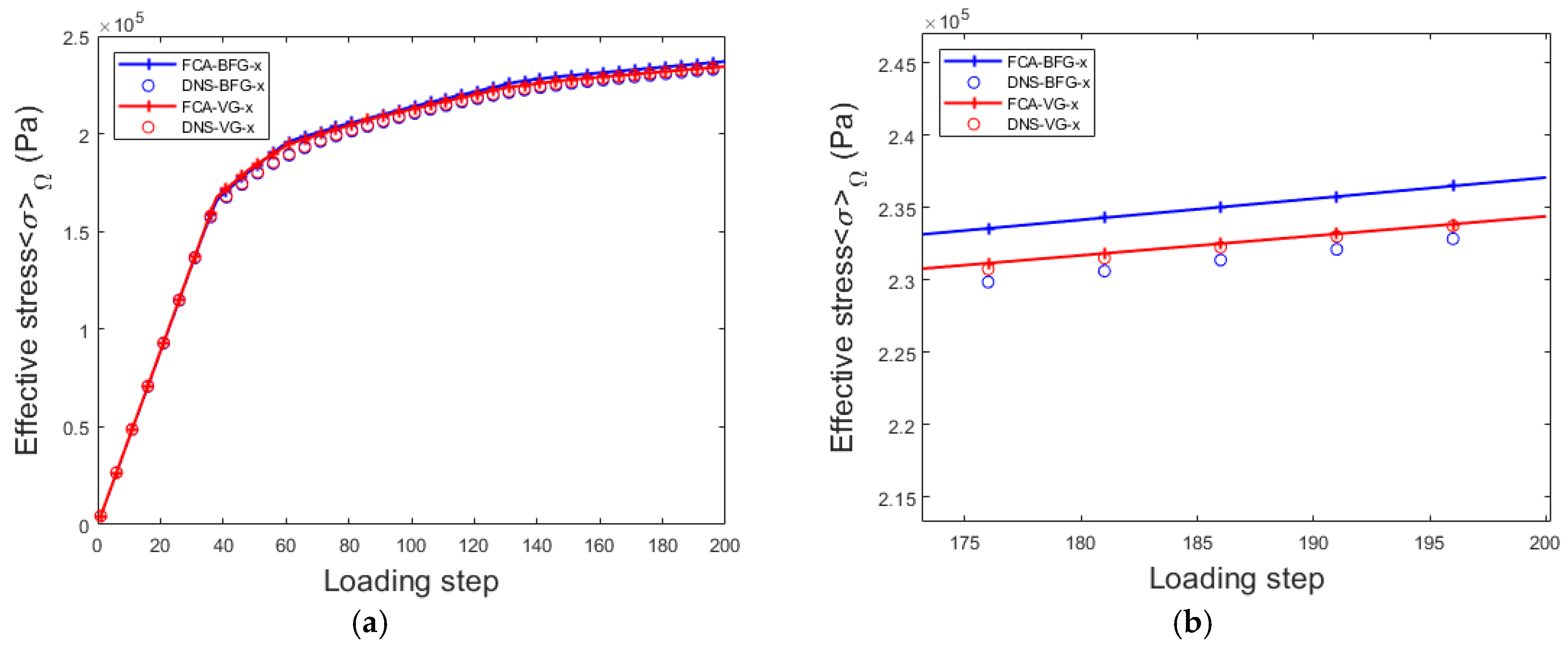
4.3. Comparative Analysis Using Voxel Elements
5. Conclusions and Outlooks
- (1)
- Unlike prior investigations on fiber- and particle-reinforced composites, complex micro structured lattice materials were constructed using parametric modeling methods. FCA was used to rapidly determine the differences in the effective stiffness and stress–strain curves of the lattice materials for different parameter values. By integrating the effective stiffness matrix, elastic modulus anisotropy diagrams are generated to clarify the effective stiffness and microstructural anisotropy characteristics of lattice materials from a micromechanical perspective;
- (2)
- Through extensive RVE examples of complex microstructure lattice materials, the effectiveness of the FCA in predicting complex microstructure lattice materials was validated by combining offline and online algorithms. The accuracy and efficiency of the FCA were compared with those of the DNS, thereby further highlighting its advantages;
- (3)
- In this study, the differences in FCA prediction outcomes between voxel and non-voxel models were investigated. For lattice materials with the same microstructure and porosity, online FCA calculations based on voxel modeling can achieve more accurate and effective attribute estimation.
Author Contributions
Funding
Institutional Review Board Statement
Informed Consent Statement
Data Availability Statement
Conflicts of Interest
Abbreviations
| FCA | FEM-Cluster-based Analysis |
| DNS | Direct Numerical Simulation |
| RVE | Representative Volume Element |
| NIAH | Novel Implementation of Asymptotic Homogenization |
| FEM | Finite Element Method |
| FFT | Fast Fourier Transform |
| POD | Proper Orthogonal Decomposition |
| PGD | Proper Generalized Decomposition |
| TFA | Transformation Field Analysis |
| NTFA | Nonuniform Transformation Field Analysis |
| SCA | Self-consistent Clustering Analysis |
| VCA | Virtual Clustering Analysis |
| DNN | Deep Neural Network |
| LSTM | Long Short-Term Memory |
| PCMCE | Principle of Cluster Minimum Complementary Energy |
| 2D | Two-dimensional |
| 3D | Three-dimensional |
| FEA | Finite Element Analysis |
| VG | Voxel Grid |
| BFG | Body-fitted Grid |
Nomenclature
| Stress | |
| Strain | |
| The matrix domain | |
| The pore domain | |
| The entire domain | |
| Displacement | |
| The corresponding boundary differential part | |
| The increment of porous strain energy and effective stress | |
| The elastic stiffness matrix | |
| Nonlinear function | |
| The parameters corresponding to various plastic strengthening criteria | |
| The mechanical strain | |
| Eigenstrain | |
| The strain concentration tensor | |
| The total stiffness matrix of the RVE | |
| The nodes displacement vector | |
| The “external force” vector applied at the nodes of the RVE | |
| The elastic microscopic strain | |
| The homogeneously elastic macroscopic strain | |
| Minimizing the total distance | |
| The strain concentration tensor for the e-th element | |
| The average strain concentration tensor for all elements in the -th cluster | |
| The total number of clusters | |
| Interaction matrix | |
| Interaction matrix components | |
| The stress vectors of each cluster in the cluster model | |
| The eigenstrain of the unit cluster under the applied working condition | |
| The singular value matrix | |
| The orthogonal matrices of the singular vectors of matrix | |
| Reconstructed interaction matrix | |
| Column vector | |
| Elastoplastic compliance matrix | |
| The volume diagonal matrix of each cluster | |
| The stress increment of step | |
| The stress of step | |
| The stress increment of step k + 1 | |
| The relative density | |
| The volume of the internal struts that form the lattice microstructure | |
| The envelope volume enclosed by the external boundary of the lattice microstructure | |
| The radius of the framework | |
| The diameter of the struts | |
| The aspect ratios | |
| The volume of the external frame | |
| Anisotropy index |
Appendix A
References
- Zhu, J.-H.; Zhang, W.-H.; Xia, L. Topology Optimization in Aircraft and Aerospace Structures Design. Arch. Comput. Methods Eng. 2016, 23, 595–622. [Google Scholar] [CrossRef]
- Evans, A.G.; Hutchinson, J.W.; Fleck, N.A.; Ashby, M.F.; Wadley, H.N.G. The Topological Design of Multifunctional Cellular Metals. Prog. Mater. Sci. 2001, 46, 309–327. [Google Scholar] [CrossRef]
- Plocher, J.; Panesar, A. Review on Design and Structural Optimisation in Additive Manufacturing: Towards Next-Generation Lightweight Structures. Mater. Des. 2019, 183, 108164. [Google Scholar] [CrossRef]
- Ashby, M.F.; Bréchet, Y.J.M. Designing Hybrid Materials. Acta Mater. 2003, 51, 5801–5821. [Google Scholar] [CrossRef]
- Yin, S.; Wu, L.; Ma, L.; Nutt, S. Pyramidal Lattice Sandwich Structures with Hollow Composite Trusses. Compos. Struct. 2011, 93, 3104–3111. [Google Scholar] [CrossRef]
- Yan, H.; Yang, X.; Lu, T.; Xie, G. Convective Heat Transfer in a Lightweight Multifunctional Sandwich Panel with X-Type Metallic Lattice Core. Appl. Therm. Eng. 2017, 127, 1293–1304. [Google Scholar] [CrossRef]
- Makarov, V.V.; Moskalenko, O.I.; Koronovskii, A.A.; Hramov, A.E.; Balanov, A.G. High-Frequency Impedance and Absorption of a Semiconductor Lattice upon an External Periodic Perturbation. Bull. Russ. Acad. Sci. Phys. 2012, 76, 1316–1318. [Google Scholar] [CrossRef]
- da Silva, A.R.; Mareze, P.; Brandão, E. Simulating Sound Absorption in Porous Material with the Lattice Boltzmann Method. J. Acoust. Soc. Am. 2014, 136, 2141. [Google Scholar] [CrossRef]
- Jin, Z.-H. A Microlattice Material with Negative or Zero Thermal Expansion. Compos. Commun. 2017, 6, 48–51. [Google Scholar] [CrossRef]
- Chan, Y.-C.; Shintani, K.; Chen, W. Robust Topology Optimization of Multi-Material Lattice Structures Under Material and Load Uncertainties. Front. Mech. Eng. 2019, 14, 141–152. [Google Scholar] [CrossRef]
- Eshelby, J.D. The Determination of the Elastic Field of an Ellipsoidal Inclusion, and Related Problems. Proc. R. Soc. Lond. A 1957, 241, 376–396. [Google Scholar] [CrossRef]
- Hill, R. Elastic Properties of Reinforced Solids: Some Theoretical Principles. J. Mech. Phys. Solids 1963, 11, 357–372. [Google Scholar] [CrossRef]
- Hill, R. A Self-Consistent Mechanics of Composite Materials. J. Mech. Phys. Solids 1965, 13, 213–222. [Google Scholar] [CrossRef]
- Hashin, Z.; Shtrikman, S. On Some Variational Principles in Anisotropic and Nonhomogeneous Elasticity. J. Mech. Phys. Solids 1962, 10, 335–342. [Google Scholar] [CrossRef]
- Hashin, Z.; Shtrikman, S. A Variational Approach to the Theory of the Elastic Behaviour of Polycrystals. J. Mech. Phys. Solids 1962, 10, 343–352. [Google Scholar] [CrossRef]
- Willis, J.R. Variational and Related Methods for the Overall Properties of Composites. In Advances in Applied Mechanics; Yih, C.-S., Ed.; Elsevier: Amsterdam, The Netherlands, 1981; Volume 21, pp. 1–78. [Google Scholar]
- Drugan, W.J.; Willis, J.R. A Micromechanics-Based Nonlocal Constitutive Equation and Estimates of Representative Volume Element Size for Elastic Composites. J. Mech. Phys. Solids 1996, 44, 497–524. [Google Scholar] [CrossRef]
- Bakhvalov, N.; Panasenko, G. Homogenisation: Averaging Processes in Periodic Media; Mathematics and its Applications; Springer: Dordrecht, The Netherlands, 1989; Volume 36, ISBN 978-94-010-7506-0. [Google Scholar]
- Cheng, G.-D.; Cai, Y.-W.; Xu, L. Novel Implementation of Homogenization Method to Predict Effective Properties of Periodic Materials. Acta Mech. Sin. 2013, 29, 550–556. [Google Scholar] [CrossRef]
- Yan, J.; Zhang, C.; Li, X.; Xu, L.; Fan, Z.; Sun, W.; Wang, G.; Yan, K. Multiscale Analysis of Bi-Layer Lattice-Filled Sandwich Structure Based on NIAH Method. Materials 2022, 15, 7710. [Google Scholar] [CrossRef]
- Pecullan, S.; Gibiansky, L.V.; Torquato, S. Scale Effects on the Elastic Behavior of Periodic Andhierarchical Two-Dimensional Composites. J. Mech. Phys. Solids 1999, 47, 1509–1542. [Google Scholar] [CrossRef]
- Yan, J.; Cheng, G.; Liu, S.; Liu, L. Comparison of Prediction on Effective Elastic Property and Shape Optimization of Truss Material with Periodic Microstructure. Int. J. Mech. Sci. 2006, 48, 400–413. [Google Scholar] [CrossRef]
- Hollister, S.J.; Kikuchi, N. A Comparison of Homogenization and Standard Mechanics Analyses for Periodic Porous Composites. Comput. Mech. 1992, 10, 73–95. [Google Scholar] [CrossRef]
- Moulinec, H.; Suquet, P. A Numerical Method for Computing the Overall Response of Nonlinear Composites with Complex Microstructure. Comput. Methods Appl. Mech. Eng. 1998, 157, 69–94. [Google Scholar] [CrossRef]
- Li, H.; Sharif Khodaei, Z.; Aliabadi, M.H. FFT-Based Homogenisation for Efficient Concurrent Multiscale Modelling of Thin Plate Structures. Comput. Mech. 2025, 75, 637–653. [Google Scholar] [CrossRef]
- Zhang, J.; Zhou, X.; Yang, S.; Liu, M. Equivalent Elastic-Plastic Model of BCC Lattice Structures. In Proceedings of the Computational and Experimental Simulations in Engineering; Zhou, K., Ed.; Springer Nature: Cham, Switzerland, 2024; pp. 785–791. [Google Scholar]
- Schneider, M. Lippmann-Schwinger Solvers for the Computational Homogenization of Materials with Pores. Int. J. Numer. Methods Eng. 2020, 121, 5017–5041. [Google Scholar] [CrossRef]
- Berkooz, G.; Holmes, P.; Lumley, J. The Proper Orthogonal Decomposition in the Analysis of Turbulent Flows. Annu. Rev. Fluid Mech. 2003, 25, 539–575. [Google Scholar] [CrossRef]
- Yan, K.; Liu, D.; Yan, J. Topology Optimization Method for Transient Heat Conduction Using the Lyapunov Equation. Int. J. Heat Mass Transf. 2024, 231, 125815. [Google Scholar] [CrossRef]
- Chinesta, F.; Keunings, R.; Leygue, A. The Proper Generalized Decomposition for Advanced Numerical Simulations: A Primer; SpringerBriefs in Applied Sciences and Technology; Springer International Publishing: Cham, Switzerland, 2014; ISBN 978-3-319-02864-4. [Google Scholar]
- Dvorak, G.J. Transformation Field Analysis of Inelastic Composite Materials. Proc. Math. Phys. Sci. 1992, 437, 311–327. [Google Scholar]
- Michel, J.C.; Suquet, P. Nonuniform Transformation Field Analysis. Int. J. Solids Struct. 2003, 40, 6937–6955. [Google Scholar] [CrossRef]
- Liu, Z.; Bessa, M.A.; Liu, W.K. Self-Consistent Clustering Analysis: An Efficient Multi-Scale Scheme for Inelastic Heterogeneous Materials. Comput. Methods Appl. Mech. Eng. 2016, 306, 319–341. [Google Scholar] [CrossRef]
- Wu, S.; Guo, L.; Li, Z.; Ding, J.; Zhuo, Y. A Damage-Related Adaptive Self-Consistent Clustering Analysis Method with Localized Refinement Capability for the Damage Problem of 3D Woven Composites. Compos. Sci. Technol. 2024, 257, 110814. [Google Scholar] [CrossRef]
- Tang, S.; Zhang, L.; Liu, W.K. From Virtual Clustering Analysis to Self-Consistent Clustering Analysis: A Mathematical Study. Comput. Mech. 2018, 62, 1443–1460. [Google Scholar] [CrossRef]
- Tang, S.; Miao, J. Virtual Clustering Analysis for Phase Field Model of Quasi-Static Brittle Fracture. Comput. Mech. 2024, 74, 875–888. [Google Scholar] [CrossRef]
- Kim, S.; Shin, H. Deep Learning Framework for Multiscale Finite Element Analysis Based on Data-Driven Mechanics and Data Augmentation. Comput. Methods Appl. Mech. Eng. 2023, 414, 116131. [Google Scholar] [CrossRef]
- Danoun, A.; Prulière, E.; Chemisky, Y. FE-LSTM: A Hybrid Approach to Accelerate Multiscale Simulations of Architectured Materials Using Recurrent Neural Networks and Finite Element Analysis. Comput. Methods Appl. Mech. Eng. 2024, 429, 117192. [Google Scholar] [CrossRef]
- Cheng, G.; Li, X.; Nie, Y.; Li, H. FEM-Cluster Based Reduction Method for Efficient Numerical Prediction of Effective Properties of Heterogeneous Material in Nonlinear Range. Comput. Methods Appl. Mech. Eng. 2019, 348, 157–184. [Google Scholar] [CrossRef]
- Nie, Y.; Cheng, G.; Li, X.; Xu, L.; Li, K. Principle of Cluster Minimum Complementary Energy of FEM-Cluster-Based Reduced Order Method: Fast Updating the Interaction Matrix and Predicting Effective Nonlinear Properties of Heterogeneous Material. Comput. Mech. 2019, 64, 323–349. [Google Scholar] [CrossRef]
- Nie, Y.; Li, Z.; Cheng, G. Efficient Prediction of the Effective Nonlinear Properties of Porous Material by FEM-Cluster Based Analysis (FCA). Comput. Methods Appl. Mech. Eng. 2021, 383, 113921. [Google Scholar] [CrossRef]
- Mandel, J. Contribution Théorique à l’étude de l’écrouissage et Des Lois de l’écoulement Plastique. In Proceedings of the Applied Mechanics; Görtler, H., Ed.; Springer: Berlin/Heidelberg, Germany, 1966; pp. 502–509. [Google Scholar]
- Zhou, X.-Y.; Gosling, P.D.; Pearce, C.J.; Kaczmarczyk, Ł.; Ullah, Z. Perturbation-Based Stochastic Multi-Scale Computational Homogenization Method for the Determination of the Effective Properties of Composite Materials with Random Properties. Comput. Methods Appl. Mech. Eng. 2016, 300, 84–105. [Google Scholar] [CrossRef]
- Chen, K.; Qin, H.; Ren, Z. Establishment of the Microstructure of Porous Materials and Its Relationship with Effective Mechanical Properties. Sci. Rep. 2023, 13, 18064. [Google Scholar] [CrossRef]
- Wang, A.-J.; McDowell, D.L. Effects of Defects on In-Plane Properties of Periodic Metal Honeycombs. Int. J. Mech. Sci. 2003, 45, 1799–1813. [Google Scholar] [CrossRef]
- Wang, C.; Zhu, J.; Zhang, W.; Li, S.; Kong, J. Concurrent Topology Optimization Design of Structures and Non-Uniform Parameterized Lattice Microstructures. Struct. Multidiscip. Optim. 2018, 58, 35–50. [Google Scholar] [CrossRef]
- Wang, C.; Gu, X.; Zhu, J.; Zhou, H.; Li, S.; Zhang, W. Concurrent Design of Hierarchical Structures with Three-Dimensional Parameterized Lattice Microstructures for Additive Manufacturing. Struct. Multidiscip. Optim. 2020, 61, 869–894. [Google Scholar] [CrossRef]
- Vaissier, B.; Pernot, J.-P.; Chougrani, L.; Véron, P. Parametric Design of Graded Truss Lattice Structures for Enhanced Thermal Dissipation. Comput.-Aided Des. 2019, 115, 1–12. [Google Scholar] [CrossRef]
- Li, Z.; Nie, Y.; Cheng, G. Mathematical Foundations of FEM-Cluster Based Reduced Order Analysis Method and a Spectral Analysis Algorithm for Improving the Accuracy. Comput. Mech. 2022, 69, 1347–1363. [Google Scholar] [CrossRef]
- Nie, Y.; Li, Z.; Gong, X.; Cheng, G. Fast Construction of Cluster Interaction Matrix for Data-Driven Cluster-Based Reduced-Order Model and Prediction of Elastoplastic Stress-Strain Curves and Yield Surface. Comput. Methods Appl. Mech. Eng. 2024, 418, 116480. [Google Scholar] [CrossRef]
- Ranganathan, S.I.; Ostoja-Starzewski, M. Universal Elastic Anisotropy Index. Phys. Rev. Lett. 2008, 101, 055504. [Google Scholar] [CrossRef]
- Li, D.; Liao, W.; Dai, N.; Xie, Y. Comparison of Mechanical Properties and Energy Absorption of Sheet-Based and Strut-Based Gyroid Cellular Structures with Graded Densities. Materials 2019, 12, 2183. [Google Scholar] [CrossRef] [PubMed]
- Momeni, K.; Mofidian, S.M.M.; Bardaweel, H. Systematic Design of High-Strength Multicomponent Metamaterials. Mater. Des. 2019, 183, 108124. [Google Scholar] [CrossRef]
- Davami, K.; Mohsenizadeh, M.; Munther, M.; Palma, T.; Beheshti, A.; Momeni, K. Dynamic Energy Absorption Characteristics of Additively-Manufactured Shape-Recovering Lattice Structures. Mater. Res. Express 2019, 6, 045302. [Google Scholar] [CrossRef]


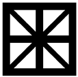
| Parameter | Microstructure | Effective Elastic Matrix (MPa) | Elastic Modulus Anisotropy Diagram (MPa) | |
|---|---|---|---|---|
 | FCA |  | ||
| NIAH | − | |||
 | FCA | 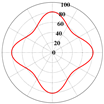 | ||
| NIAH | − | |||
 | FCA | 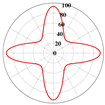 | ||
| NIAH | − | |||
| FCA | DNS | |
|---|---|---|
| Number of degrees of freedom | 120 | 29,282 |
| Computational time (one step) | 0.003 s | 1.179 s |
| Contrast | 393 times | - |
| Parameter | Microstructure | Effective Elastic Matrix (MPa) | Elastic Modulus Anisotropy Diagram | |
|---|---|---|---|---|
 | FCA |  | ||
| NIAH | − | |||
 | FCA |  | ||
| NIAH | − | |||
 | FCA | 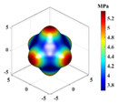 | ||
| NIAH | − | |||
 | FCA | 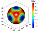 | ||
| NIAH | − | |||
 | FCA | 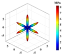 | ||
| NIAH | − | |||
 | FCA |  | ||
| NIAH | − | |||
| FCA | DNS | |
|---|---|---|
| Number of degrees of freedom | 180 | 332,787 |
| Computational time | 0.277 s | 3241.7 s |
| Contrast | 11,702 times | - |
Disclaimer/Publisher’s Note: The statements, opinions and data contained in all publications are solely those of the individual author(s) and contributor(s) and not of MDPI and/or the editor(s). MDPI and/or the editor(s) disclaim responsibility for any injury to people or property resulting from any ideas, methods, instructions or products referred to in the content. |
© 2025 by the authors. Licensee MDPI, Basel, Switzerland. This article is an open access article distributed under the terms and conditions of the Creative Commons Attribution (CC BY) license (https://creativecommons.org/licenses/by/4.0/).
Share and Cite
Yan, J.; Liu, Z.; Liu, H.; Zhang, C.; Nie, Y. Rapid Prediction of Nonlinear Effective Properties of Complex Microstructure Lattice Materials. Materials 2025, 18, 1301. https://doi.org/10.3390/ma18061301
Yan J, Liu Z, Liu H, Zhang C, Nie Y. Rapid Prediction of Nonlinear Effective Properties of Complex Microstructure Lattice Materials. Materials. 2025; 18(6):1301. https://doi.org/10.3390/ma18061301
Chicago/Turabian StyleYan, Jun, Zhihui Liu, Hongyuan Liu, Chenguang Zhang, and Yinghao Nie. 2025. "Rapid Prediction of Nonlinear Effective Properties of Complex Microstructure Lattice Materials" Materials 18, no. 6: 1301. https://doi.org/10.3390/ma18061301
APA StyleYan, J., Liu, Z., Liu, H., Zhang, C., & Nie, Y. (2025). Rapid Prediction of Nonlinear Effective Properties of Complex Microstructure Lattice Materials. Materials, 18(6), 1301. https://doi.org/10.3390/ma18061301