Article

Small-Scale Hybrid Methanol–Methane Production Based on Biogas: Stochastic Sensitivity Analysis of the Economic Sustainability

by
Rosa Zuloeta Bonilla
* and
Ramchandra Bhandari
*
Institute for Technology and Resources Management in the Tropics and Subtropics, TH Köln–University of Applied Sciences, Betzdorfer Strasse 2, 50679 Cologne, Germany
*
Authors to whom correspondence should be addressed.
Energies 2022, 15(24), 9329; https://doi.org/10.3390/en15249329
Submission received: 8 November 2022 / Revised: 5 December 2022 / Accepted: 6 December 2022 / Published: 9 December 2022
(This article belongs to the Special Issue New Trends in Biofuels and Bioenergy for Sustainable Development)

Abstract

:
This study investigates the economic viability at the pre-feasibility level of a hybrid methanol and biomethane plant based on biogas coupled to a photovoltaic (PV) power plant and a proton exchange membrane (PEM) electrolyzer. The reference case settled in Uganda consisted of two units powered by a 200 kW PV plant and grid power: a 25 Nm3/h anaerobic digester and a 140 kW PEM electrolyzer-based methanol plant. Its production of 33.3 tons of methanol and 70.1 tons of biomethane per year can provide cooking fuel for 750 households. Response Surface Methodology was used to evaluate the impact of the three main factors on the simple payback period (PBP). The size of the PV plant had the most significant impact on PBP, followed by the cost of electricity, the interaction between these factors, and the PEM electrolyzer capital cost reduction, in this contribution order. These findings point to energy generation costs as the primary factor affecting the economic viability of these small-scale designs, even more than the PEM’s capital cost. The response surface analysis revealed that only in a reduced region of the design space are values found that meet the threshold of 10 years for plant economic viability.

1. Introduction

Transitioning to cooking fuels and technologies that meet the World Health Organization’s Indoor Air Quality Guidelines aims to prevent enormous health, environmental, and economic impacts resulting from the burning of polluting fuels for cooking, mainly in low- and middle-income countries [1]. The universal energy access process is accelerated by deploying sectoral frameworks and engagement plans [2]. Large-scale clean cooking intervention programs across Asia, Africa, and Latin America have adopted cleaner fuels such as biogas, liquefied petroleum gas (LPG), alcohol-based (ethanol and methanol), electricity, and processed biomass fuels (briquettes and pellets) [3]. Biogas holds the lowest levelized annual cooking cost among the clean cooking technology options, and only solar cook stoves match its health and climate impact indicators [4]. Despite its advantages, household biogas production for cooking encounters significant barriers to uptake, even generating the dis-adoption of biogas technologies [5,6,7]. High installation costs (between USD 500–1500 depending on the type of digester) are only affordable for 20–30% of households in South Asian, Southeast Asian, and African regions [4]. The technical skills shortages and the challenge of biogas product and service markets to emerge in tandem with biogas programs are recurring barriers to the installation, operation, and maintenance of domestic biogas systems [8]. Moreover, cultural and social taboos concerning animal use, especially human waste, may discourage its adoption in specific contexts [9].
This study focuses on small-scale decentralized biogas-derived fuel production to unlock the potential of biogas as clean cooking fuel where biogas distributed generation fails to be sustainable long-term. In this model, the substrate is disposed of at a decentralized and technically advanced biogas plant to obtain clean fuels or fertilizers [10]. We hypothesize that the so-called power-to-fuel technologies could significantly address household biogas production disadvantages by converting carbon dioxide and hydrogen into synthetic organic molecules. Synthetic products exhibit similar properties to fossil fuels so they can be transported commercially in metal tanks or liquid at atmospheric pressure and profit from existing cookstoves [11]. This study analyzes the economic viability of hybrid methanol and methane production based on biogas at the pre-feasibility and small-scale levels.
This work contributes to the only publication by Moioli, Wötzel, and Schildhauer that assesses the economics of hybrid methanol and methane production components based on biogas. Moioli et al. investigated the economic prospects of a hybrid Power-to-Methanol/Power-to-Gas system for the first time, i.e., coupling methanol production with biogas upgrading [12]. In contrast to their approach, which involves CO2 hydrogenation reaction to methane and methanol, we integrate power into methanol technology to valorize the removed carbon dioxide from biogas upgrading. Capitalizing on existing modular technology, we intend to determine whether the benefits of generating clean biogas-based fuels for upgrading or transforming into synthetic fuels can also be accessible in LMICs as a cooking fuel. Indeed, hydrogen as a clean fuel to substitute polluting cooking fuels in LMICs is not a novel idea, e.g., [13,14,15]. Its application, however, is currently infeasible due to cost, complexity, lack of labor capacity, safety issues, and consumer acceptance [16]. Nonetheless, hydrogen penetration in the residential sector of LMICs might occur progressively without the need for disruption or change in appliances in the form of synthesized fuels.
The study’s purpose is to answer these two questions: (1) What is the simple payback period for a small-scale hybrid methanol and methane plant whose products are sold at a price equivalent to LPG’s cooking cost? (2) What factors strongly influence the economic viability of this system? This paper uses sensitivity analysis to offer a comprehensive economic outline of the problem based on the Response Surface Methodology. We use this approach to determine whether a proposed design would be profitable under certain economic conditions. With varying parameters such as electrical energy, PV plant size, and components capital costs, the simple payback period (PBP) is investigated by combining the mentioned parameters in different ways.
The study is set in Uganda, an agricultural country with plentiful food and cash crop cultivation year in and year out [17,18]. Its abundant biogas potential from crop and animal residues favored its inclusion in the Africa Biogas Partnership Program [7]. Nevertheless, the massification of household biodigesters has faced drawbacks in the uptake, leading to high levels of dis-adoption within four years after its installation [5]. The economic analysis of a 25 Nm3/h of raw biogas plant attempts to reflect the energy system’s performance in this context.

2. Background on Clean Cooking Fuels

The WHO-IAQG has provided normative recommendations in carbon monoxide (CO) and particulate matter (PM2.5) emission-rate targets for the set fuel-cooking technologies to prevent adverse health outcomes and climate impacts [1]. Cooking solutions should perform under the interim target-1 (IT-1) and the WHO’s air quality guideline (AQG) for an annual mean PM2.5 of 35 µg m−3 and 10 µg m−3, respectively, and the 24 h average AQG for carbon monoxide (CO) of 7 mg m−3 [19,20]. These parameters draw the line between clean and polluting fuels, i.e., those that comply with them and those that do not.
According to the WHO’s IAQG-Review 6, despite achieving significant reductions in PM2.5 compared to solid fuels with traditional stoves (30–60%), none of the enhanced solid fuel stoves tested met the WHO IT-1 for PM2.5 annual mean, thus, failing to meet the AQGs [21,22]. Later, these findings were revalidated and disclosed that neither advanced combustion stove met WHO-IT-1, even though pellet-fueled stoves were not documented [23]. Kerosene may not be superior to solid fuels in health impacts [24,25], so the WHO discourages its use as well [1]. Accordingly, polluting fuels are unprocessed biomass (crop residues, wood, and animal dung), kerosene, coal, and charcoal (Figure 1). In contrast, studies reporting alcohol-based, liquefied petroleum gas and electricity interventions reported mean PM2.5 concentrations close to or at IT-1 levels, and most achieved the WHO 24 h guideline level [23]. Biogas cookstove assessments also demonstrate notable reductions in HAP exposures and improved health outcomes [4]. Therefore, clean fuels consist of petrochemical fuels (such as LPG and natural gas), grid electricity, and renewable fuels (such as biogas, alcohol-based, and solar photovoltaic electricity) (see Figure 1). This study focuses on methane and methanol, clean cooking fuels that have been demonstrated to displace polluting practices in the households of LMICs and whose broad scale-up is now in motion in many countries.

3. Methods

In stochastic systems, the Design of Experiments (DoE) methods are used to analyze the influence of multiple independent variables (factors) on dependent variables (responses). The analysis of experimental studies involves applying the analysis of variance (ANOVA) models that determine and quantify the influence of factors or their interactions on the observed response of an experiment and whether these interactions result from randomness or a specific cause [26]. The sample is a series of experimental runs that compromises the experimental design [27]. In an experimental design, the term block describes a group of experimental units with some similarities. The blocking reduces known but irrelevant sources of variation between experiments, allowing for a more precise estimation of the various sources. Some experiments may be replicates, meaning they were conducted under the same conditions. Groups within a sample are a set of runs associated with a particular factor, level, and interaction. The ANOVA method decomposes the total variance into its various components by comparing the means and variance of the groups [28]. Thus, quantifying the effects of various predictors (factors and interactions) on the dependent variables is possible.
The Response Surface Methodology (RSM) is a potent DoE optimization tool pioneered by Box and Wilson in 1951 [29] that seeks to determine the optimal design (the grid of candidate points) for building regression models relative to the objective function.

3.1. ANOVA Analysis

This analysis determines whether the interactions and effects between the investigated factors are statistically significant concerning an experimental error. ANOVA proceeds by first estimating these effects for individual factors and possible interactions; then, the significance of these effects is inferred [26]. Statistical significance is tested by Fischer’s variance ratio (F-value), and model terms are either rejected or selected based on the significant probability value (p-value) within a 95% confidence interval (or 5% significance level). Additionally, graphical methods are employed for examining model fit.

3.2. Response Surface Methodology

The RSM approach has the following objectives: (1) to find the optimum response and (2) to understand the changes in the response in a specific direction by adjusting the design variables [29]. The model’s response is assumed to be a function of the independent variables, as indicated by Equation (1).
y = f ( x 1 ,   x 2 , ,   x k ) + ε
In Equation (1), y represents the response variable, x 1 ,   x 2 , ,   x k are the independent variables, and ε stands for the normally distributed experimental error, i.e., N ( 0 , σ 2 ) [30]. The expected value of the output is:
E ( y ) = η
η is the expected response surface.
Either first-order or second-order models are used, depending on the approximation of the f function. If a linear regression equation can define the response, then the estimating function is a first-order regression model. Equation (3) represents k factors generating a single response y . β 0 is a constant and β i are linear terms.
y = β 0 + i = 1 k β i x i + ε
However, the first-order model is insufficient when a curvature in the response surface exists. Therefore, the second-order model helps approximate a portion of the actual response surface with curvature. It is represented in Equation (4).
y = β 0 + i = 1 k β i x i + i < j k β i j x i x j + i = 1 k β i i x i 2 + ε
where β 0 is a constant, β i are linear terms, β i j are interaction terms, and β i i are quadratic terms.
The model’s accuracy may need to be improved by reducing the gap between Predicted R2 and Adjusted R2. By excluding non-significant regression coefficients, this can be achieved.

Experimental Design for Fitting Response Surfaces

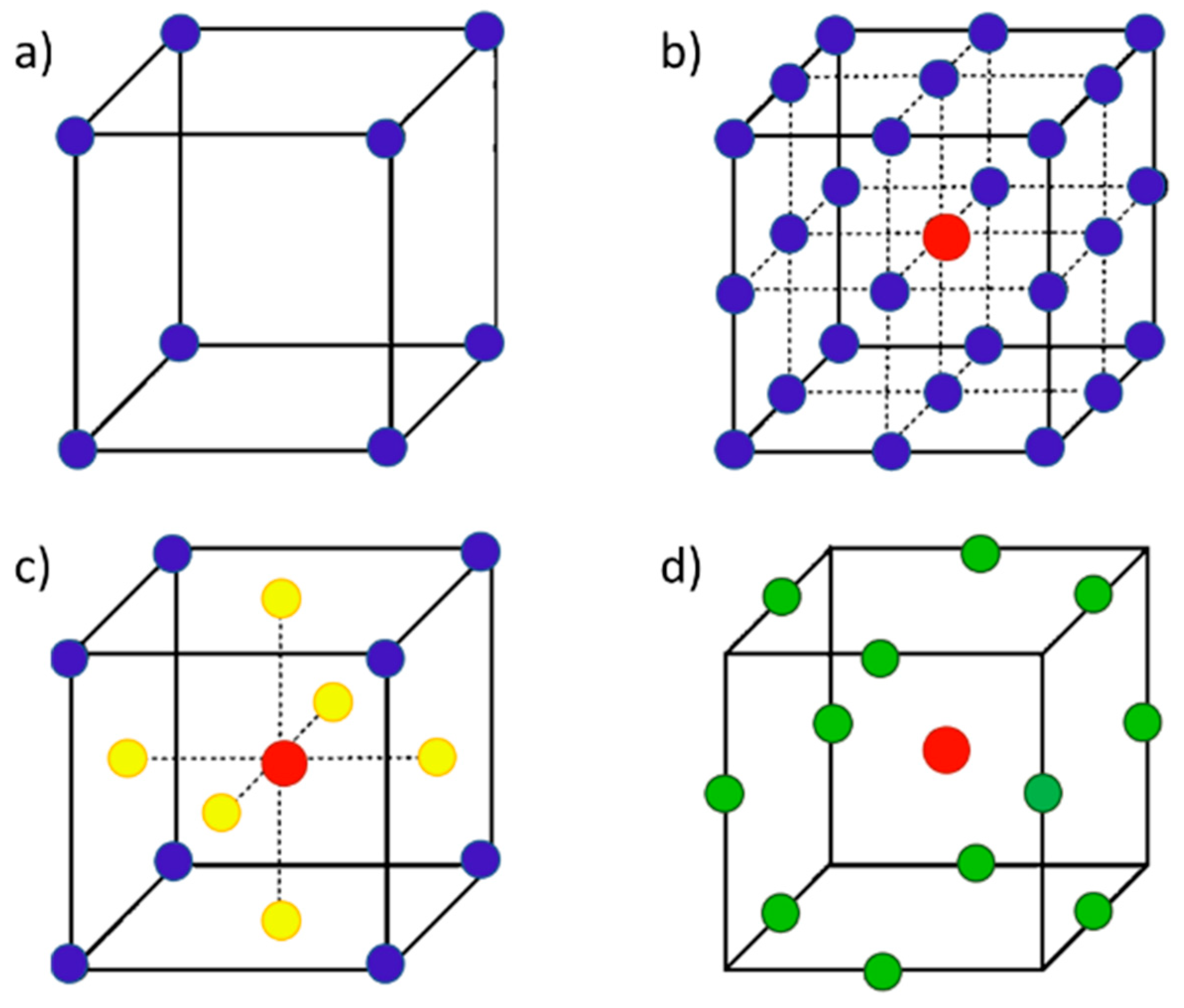
The experiments in response surface designs are special cases of factorial design that include center points in the experimental space plus edge center points or face center points and extra points circumscribed from the sides. Each experimental run in a factorial design consists of a combination of levels ( l ) for each factor, resulting in l k experimental runs. Usually, factorial designs are two-level designs, that is, one high and one low value is used for each factor. A full factorial design requires that every combination of every factor is run at every level. For instance, a two-level full factorial design and three factors (Figure 2a) result in 23 experimental runs. These designs can become very large as the factors increase, e.g., a three-level full factorial design (Figure 2b).
Response surface designs are used when multi-factors have been identified, and improved descriptions of their curvature and interactions are needed [31]. There are two main types of response surface designs: Box–Behnken and Central Composite designs. Box–Behnken designs (Figure 2d) have fewer experimental runs, but interactions between factors at the ‘extreme’ levels (i.e., the ‘corners’) are not accounted for. Central Composite designs, also known as Box–Wilson designs, merge factorial designs with ‘star points’ for estimating second-order effects. They are described as inscribed, circumscribed, or face-centered depending on whether the axial points fall within, beyond, or on the factorial space. Compared to circumscribed and inscribed, which require five levels of each factor, face-centered (Figure 2c) requires three levels, thus, simpler to run, and reasonably describes the entire design space. This study employs Version 13 of Design-Expert software (DX13) to explore the factor(s) influencing the response(s) investigated in the proposed plant by analyzing a Face-Centered Central Composite design (Figure 2c).

4. Plant Layout Description

Figure 3 displays the conceptual block diagram of the system under investigation. Raw biogas is produced from the anaerobic digestion of organic materials from manure and straw. Biogas is processed through biogas cleaning and upgrading to increase energy density by separating hydrogen sulfide and carbon dioxide from biomethane. Methanol is synthesized based on carbon dioxide generated from the upgrading process and hydrogen produced by a PEM water electrolyzer. A PV power plant is installed to supply the electrical energy for methanol and methane production. Purchasing the necessary electricity from the grid is assumed when solar energy is unavailable. Thus, the PEM water electrolyzer can switch between solar energy and grid electricity (and vice versa) without affecting its functionality [32]. The plant is expected to operate 7900 h per year (90% operating factor), a value within the recommended range to yield lower production costs for the methanol synthesis unit and the PEM electrolyzer [33,34]. Next, a description of the system’s main components under investigation is given.

4.1. Anaerobic Digestion

Anaerobic digestion is the process by which bacteria break down organic matter—such as wastewater biosolids, animal manure, and food wastes—in the absence of oxygen. This study analyses a plant with the capacity to produce 25 Nm3/h of raw biogas whose product has a proportion of 54% CH4, 46% CO2, and 220 ppm H2S—an average composition in several biodigesters in Uganda [6]. The agricultural residue required to produce 1 Nm3 of raw biogas is approximately 12 kg [35].

4.2. Biogas Cleaning and Upgrading

Water scrubbing is applied to remove CO2 from biogas as it is effective even at low flow rates where small-scale biogas plants operate. Since CH4 is significantly less soluble in water than CO2, water serves as a solvent in water scrubbing [36]. By removing more CO2 from the biogas flow in the absorption column, the concentration of CH4 in the biogas increases. Even though H2S can also be disposed of with CO2, dissolved in water, it can cause corrosion problems in downstream applications; therefore, pre-separation thorough cleaning is necessary. It is assumed that the CH4 losses, mainly due to dissolution in water, are usually lower than 2% [37], and the purity of CO2 can achieve up to 80–90% [38]. This study’s reference design is the water-scrubbing system designed by Engas UK Ltd. for use in small biogas production facilities because of modularity and flexibility. Its technical specifications are listed in Table 1. This technology combines the three key phases of water scrubbing. That is, the pre-compression, scrubbing, and drying of biogas [39]. After absorption, the water used is regenerated in a desorption column under air, which strips the CO2 from the water under reduced pressure. Finally, the CO2 is compressed to feed the methanol synthesis unit.

4.3. Methanol Synthesis Unit

According to Equation (5), methanol is synthesized from carbon dioxide and hydrogen.
CO 2 + 3 H 2 CH 3 OH + H 2 Δ H = 49.4   kJ / mol
The streams of H2 and CO2 are mixed in a 1:3 stoichiometric ratio and sent to the reactor for methanol synthesis. Operating conditions are based on the 50 kg/day small-scale methanol synthesis plant analyzed by Ushikoshi, Mori, Watanabe, and Takeuchi [40]. The catalytic reaction is exothermic, occurring on a Cu/ZnO-based multicomponent as a catalyst over a range of temperature and pressure from 230 °C to 270 °C and from 30 bar to 70 bar, respectively. The gaseous products then pass into the distillation section to separate the water and obtain methanol in liquid form. The conversion efficiency of the reactor (expressed as the ratio of the mass of methanol produced to the mass of methanol that can theoretically be produced under stoichiometric conditions) is assumed to be 96%, and the electrical energy demand (basically for compression) is 0.154 kWh per kg of methanol [41].

4.4. PEM Water Electrolyzer

A PEM electrolyzer is a device that produces oxygen and hydrogen through the water electrolysis process. The reactions involved at the anode and cathode of the electrolyzer are as follows:
Anode : 2 HO 2 O 2 + 4 H + + 4 e Catode :   4 H + + 4 e 2 H 2 Total :   HO 2 O 2 + 1 2 O 2
The relation between the mass flow rate of H2, m ˙ h , e l y (kg/h), and the electrolyzer power, P e l y (kW), is given in Equation (7) [42]:
P e l y = S P C e l y · m ˙ h , e l y
where S P C e l y (kWh/kg) is the specific power consumption of the electrolyzer, accounting for rectifier losses, auxiliary, and water splitting power. The specific power consumption of 56.7 kWh/kg for continuous hydrogen production is assumed [13].
Hydrogen production technologies based on electrolysis are currently gaining traction rapidly. The cost of hydrogen production substantially impacts electrolysis plant economics. In the current hydrogen production cost structure, the energy generation costs are the highest, followed by the capital expenditures for the electrolysis system [33]. Therefore, including the PEM’s capital cost as an independent variable in sensitivity analysis is relevant for the economic viability analysis. Based on commercial development trends and academic research activities, Holst et al. estimated around a 40% cost decrease by 2030 for decentralized, small-capacity low-temperature PEM water electrolysis systems [33]. According to this assumption, sensitivity analysis examines the impact of reductions from 0 to 40%, with existing costs as the base case.

4.5. Photovoltaic Power Plant

The photovoltaic power plant is installed to supply energy to the biomethane–methanol plant. Because Uganda’s electricity service is deficient [43], this facility is critical for the plant’s continuous operation. A photovoltaic electrolysis system can be configured in various ways, each with a different economic value. One extreme of the configurations under analysis is based on a grid connection to supplement the PV array’s electricity supply. The photovoltaics are sized such that their maximum instantaneous power matches the biomethane–methanol plant’s capacity. Grid connection is assumed in the base case analysis. At the other extreme, the PV system provides 100% of the energy required by the system. In the sensitivity analysis, this range of values shall serve to investigate the influence of the PV plant size.
The average monthly solar radiation in Eastern Uganda is the basis for calculating the PV panels’ electricity production. Monthly daily solar radiation on the horizontal surface fluctuates from 5.22 kWh/m2/day to 6.28 kWh/ m2/day between July and March, with an annual average of 5.85 kWh/ m2/day [44]. The performance ratio of the installation is assumed to be 75.84%, as reported in a facility in Uganda [44]. Table 2 summarizes the technical parameters of the sub-systems described above.

5. Economic Calculation

The Ugandan economic scenario is the reference for the thermo-economic analysis. The following sections report the main economic assumptions in the base case.

5.1. Feedstock Price

It is assumed that the feedstock for anaerobic digestion is obtainable without costs. Since agricultural producers tend to incur expenses in waste management, this assumption reflects their potential willingness to provide free feedstock in exchange for disposing waste [35].

5.2. Electricity Price

Despite the high PV plant capacity factor (16–20%), the only use of solar energy is insufficient to ensure the plant’s planned annual operating hours (7900 h). Therefore, when there is no electricity generation from the PV plant, it is required to buy it from the grid. One of the primary cost drivers for an energy system involving an electrolysis unit is the electricity cost, thus, it is essential in determining the plant’s economic viability [33]. The monthly average electrical market price for medium industrial consumers between 2019 and 2022 ranges from USD 0.115 per kWh to USD 0.149 per kWh, and the average price is equal to approximately USD 0.132 per kWh [45]. The same range is used in the sensitivity analysis to investigate the energy–cost effect. In the base case analysis, electrical energy is assumed to be purchased from the grid at USD 0.115 per kWh.

5.3. Products Selling Price

Although biogas and ethanol/methanol have the lowest environmental impacts, neither of these fuels are currently used significantly in Uganda, and data on costs and implementation are insufficient [46,47]. Thus, methane or methanol selling prices are approximated to match the price of LPG in terms of its energy density per unit of mass (LPG energy density = 13.6 kWh/kg). This assumption is based on LPG’s lower cost than kerosene, wood fuel, pellets, and charcoal in urban and peri-urban settings [48], which would ensure the competitiveness of biomethane and methanol. Considering the energy density of the products (methane energy density equal to 12.89 kWh/kg, and methanol energy density equivalent to 6.1 kWh/kg) and that the selling price for an LPG refill in Uganda is USD 2.60 per kg [35], the selling price is assumed to be USD 2.46 per kg for methane and USD 1.17 per kg for methanol. In addition, the trading of oxygen produced by the electrolyzer is central to the plant’s economic viability. The refilling oxygen price is assumed to be USD 0.130 per kg, the reference price for medical oxygen prior to the COVID-19 pandemic in Uganda, when a significant price increase was experienced due to low availability.

5.4. Purchased Equipment Cost Estimation

The sum of the capital cost of each plant component is the total Purchased Equipment Cost (PEC). The Total Capital Investment (TCI) is calculated based on the PEC of the plant: about 40% of TCI is attributed to the PEC [49]. Additionally, the TCI corresponds to the Initial Investment in this study. Table 3 presents the methods and references employed for estimating the costs associated with the hybrid methanol–methane plant.

5.5. Economic Analysis

The economic parameters such as interest rate, inflation, and taxation are not reflected for simplicity of the analysis because its primary purpose is to evaluate the parameters’ relative effect on the system’s economic viability. The simple payback period (PBP) is the investment performance measure. Despite its limitations, the PBP is widely operated as a screening measure and rule of thumb for investments. A threshold of 10 years of PBP is selected for plant economic viability, assuming a 20-year project lifetime. The PBP is calculated under Equation (8), where the annual cash inflow is expected to be constant over the plant’s lifetime.
PBP = I n i t i a l   i n v e s t m e n t A n n u a l   c a s h   i n f l o w
Equation (9) calculates the annual cash inflow.
A n n u a l   c a s h   i n f l o w = A n n u a l   p r o d u c t s   i n c o m e A n n u a l   v a r i a b l e   c o s t

6. Results and Discussion

6.1. Base Case Results

The reference case is a small-scale hybrid methanol and methane production based on biogas consisting of a 25 Nm3/h anaerobic digestor undergoing cleaning and upgrading to produce methane and a 140 kW PEM electrolyzer-based methanol plant powered by a 200 kW PV power plant and grid power supply energy to the system. In Table 4, the mass and energy balance of the plant is reported. Based on the household fuel consumption estimates for LPG users in Uganda of 14.4 MJ per day [46], 139 households could be supplied annually with methanol and 614 households with biomethane.
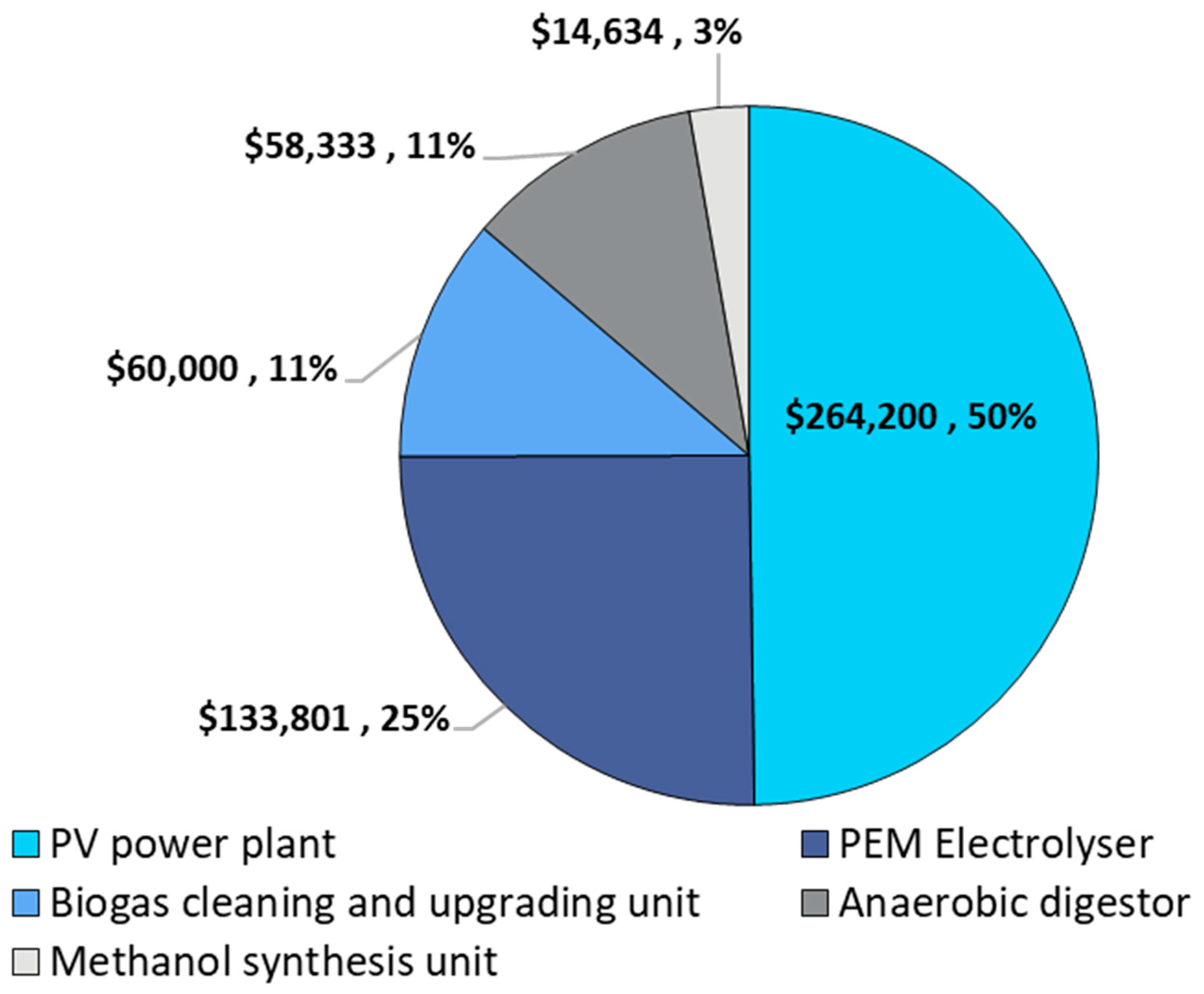
The breakdown and percentage distribution of the PEC are reported in Figure 4. Representing 50% and 25% of the PEC are the PV plant and PEM electrolyzer, the most expensive components. The biogas upgrading and anaerobic digestor unit costs equal 11% of the PEC. The methanol synthesis unit represents the lowest cost, accounting for only 3%. The resulting TCI equals about USD 1.3 million, and the annual cash inflow in Table 5 is USD 129,279; therefore, the base case presents a PBP of 10.3 years. The reference case plant has exceeded the 10-year PBP threshold, so it is not economically viable in this case. Hence, sensitivity analysis should be performed to identify the minimum PBP.
The PEC distribution results indicate that PV plant and PEM electrolyzer capital costs would strongly influence the economic viability of the proposed design. It is, therefore, pertinent to include the foreseeable reduction of up to 40% of the PEM capital cost as an independent variable in the sensitivity analysis. The different configurations of the PV plant mean that the size of the PV arrays and the grid power consumption vary. When the PV plant size is such that it matches the maximum instantaneous power demanded by the biomethane–methanol plant, the grid will supply the remaining energy. In contrast, when the PV plant generates 100% of the energy, there is no consumption from the grid. Since PV plant size is closely linked to energy grid consumption, both PV plant size and electricity prices compromising grid consumption costs should be analyzed independently.

6.2. Sensitivity Analysis Results

A quantitative mathematical model for the PBP was developed by applying the RSM. The dependent variables investigated are the size of the PV plant, the PEM’s capital cost reduction, and the electricity price, coded as variables A, B, and C, with their levels listed in Table 6. The significance test of model fit for the PBP was performed using Version 13 of Design-Expert software (DX13) based on a three-way ANOVA for the three independent variables and one response. A Face-Centered Central Composite design was applied for this purpose, resulting in 20 runs (Table 7). Replicates were generated under the minimum, average, and maximum annual solar radiation conditions from Table 2.
The ANOVA analysis verifies the significance of the different models—linear model, two-factor interaction (2FI) model, and quadratic model. Table 8 indicates the models’ statistical data. The results display that the 2FI and linear models present a p-value lower than 0.05, indicating a 95% confidence level of statistical significance. The coefficient R2 determines the variance proportion in the response that the independent variables can explain. The difference between predicted and observed values is minimal when R2 is close to 1. However, if additional terms are added, as in the case of the quadratic model in Table 8, even if they are not statistically significant, the R2 can be artificially increased. Therefore, the focus should be on the Predicted R² and Adjusted R2 values. Adding insignificant terms to the model plateaus the Adjusted R2 while the Predicted R2 decreases. As a rule of thumb, the Predicted R² and Adjusted R2 values should be within 0.2. According to the 2FI model’s values, it is most suitable for further analysis. However, the 0.7303 Predicted R² is not as close to the 0.9581 Adjusted R², i.e., a difference of 0.2278, more than 0.2. Therefore, the significance of the estimated regression terms affecting the 2FI model should be tested.

6.2.1. Statistical Evaluation of the Model

The corresponding F-test value of the ANOVA analysis can state the significance of individual model coefficients. Additionally, the significance factors can be analyzed based on the sum of squares value and their contribution. Higher values imply more importance of the corresponding factor. Table 9 shows the ANOVA table for the 2FI model for PBP. The p-value for the model is less than 0.05, which indicates the significance of the model. The effect of PV plant size (A) is the most considerable factor associated with the PBP, obtaining a sum of squares of 11.66 (48.34%). This effect was expected because the PV plant represents 50% of the PEC (Figure 4). The secondary contribution derives from the electrical energy purchasing cost (C) with 6.4 (26.53%). The third contributor is the interaction between the size of the PV plant and the energy purchasing cost (AC), whose sum of squares is 3.92 (16.25%), further highlighting their influence on the PBP. Even though the PEM is the second most expensive component representing 25% of the PEC (Figure 4), the reduction in PEM capital cost (B) with a sum of squares of 1.85 (7.76%) is ranked as the fourth contributor. Consistently, the interaction terms, PV plant size and reduction in PEM capital cost (AB) and reduction in PEM capital cost and electrical energy purchasing cost (BC), are not significant due to the non-interaction between the linear terms. Their remotion may result, therefore, in an improved model.
By adopting the backward elimination procedure to reduce the non-significant terms, the resulting fit statistics and ANOVA for the reduced 2FI model are shown in Table 10 and Table 11, respectively. Equation (10) provides the final equation for the PBP in terms of coded factors.
PBP = 12.43 + 1.08 A 0.43 B + 0.80 C 0.70 AC
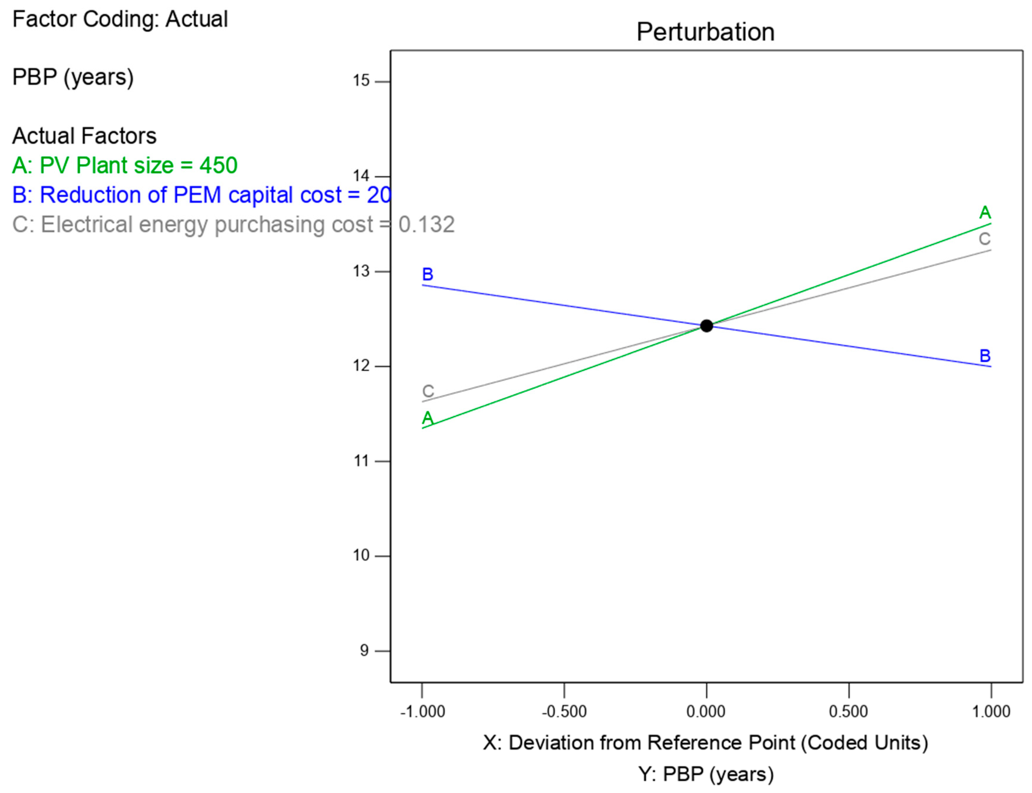
Plotting the perturbation factors allows for comparing all factors’ effects at a particular point. Figure 5 shows all factors’ effects at the design space’s midpoint. As the value of the PV plant size (A) and the electrical power purchase cost (C) increase, the PBP consequently increases. Conversely, the increasing reduction in PEM capital cost (B) decreases the response PBP. As expected, the remotion of the interaction terms AB and AC improved the model’s accuracy by reducing the difference between the Adjusted R2 (94.92%) and Predicted R2 (86.06%) to 0.0886 in Table 10. The R2 of the model indicates it can explain 98.12% of the variation in the response variable around its mean. Adequate precision in Table 10 is a signal-to-noise ratio that contrasts the predicted values range at the design points with the average prediction error. As ratios above 4 indicate adequate model discrimination, 33.257 suggests an adequate signal.
In Table 11, the high model F-value (80.48) and the model p-value of less than 0.05 confirm the model’s statistical significance. The contributions of the kept terms increased to the following values: PV plant size (A: 48.93%), reduction in PEM capital cost (B: 7.76%), electrical energy purchasing cost (C: 28.86%), and the interaction between electrical energy purchasing cost and PV plant size (AC: 16.45%). Besides the linear terms, the interaction term AC was anticipated to contribute significantly to the PBP, given the strong correlation between the amount of energy consumed from the grid and PV plant size, which impacts production costs subject to electricity prices. Interestingly, its contribution is even higher than the linear term B, indicative of its relevance to the PBP, over and above the PEM’s capital cost reduction variable. These results suggest that methanol production costs are impacted by hydrogen generation cost trends, dominated by energy generation costs, followed by the costs of electrolysis systems [33]. Even though the statistical evaluation suggests the model’s goodness of fit, it is necessary to check the residual plots to discard unwanted residual patterns.
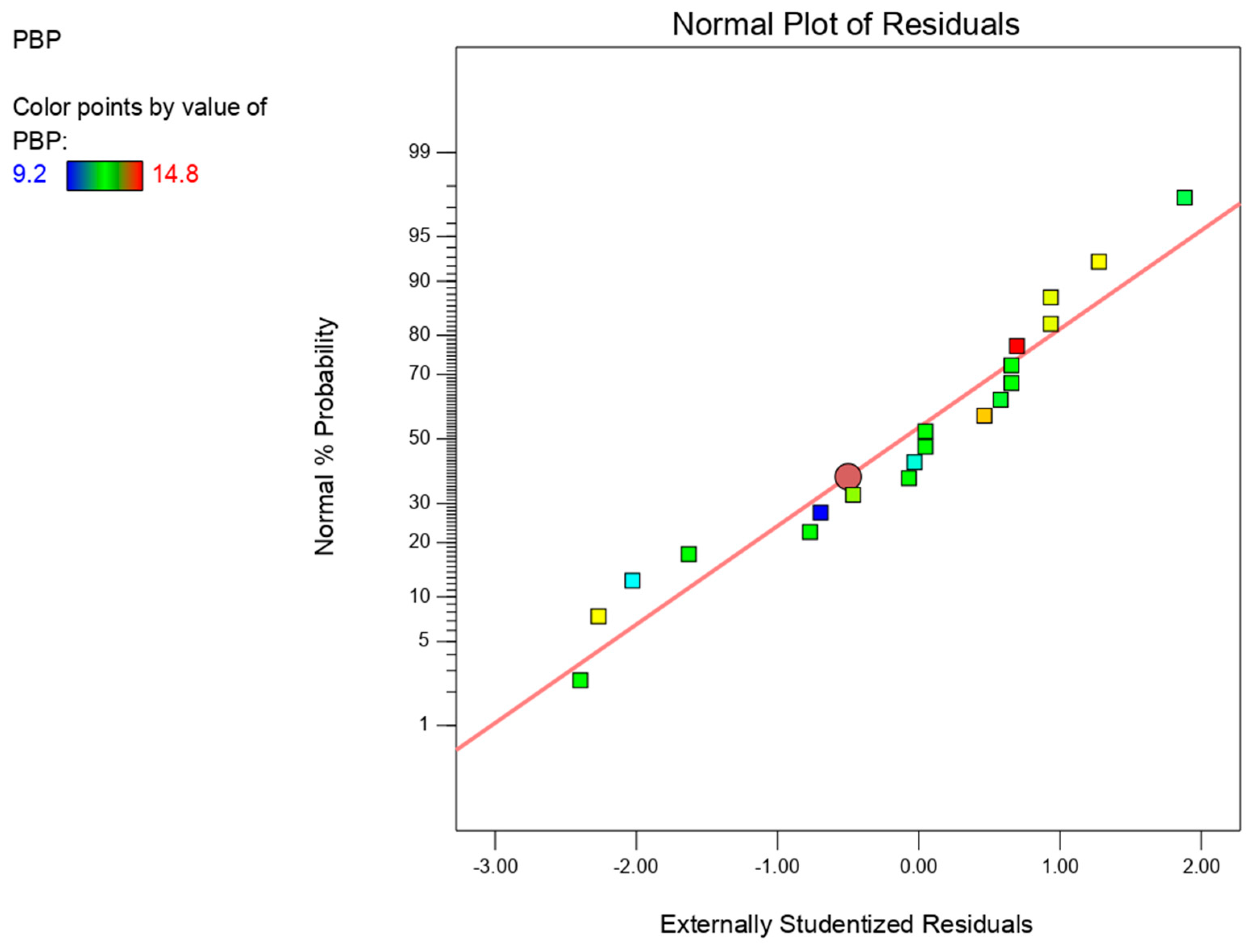
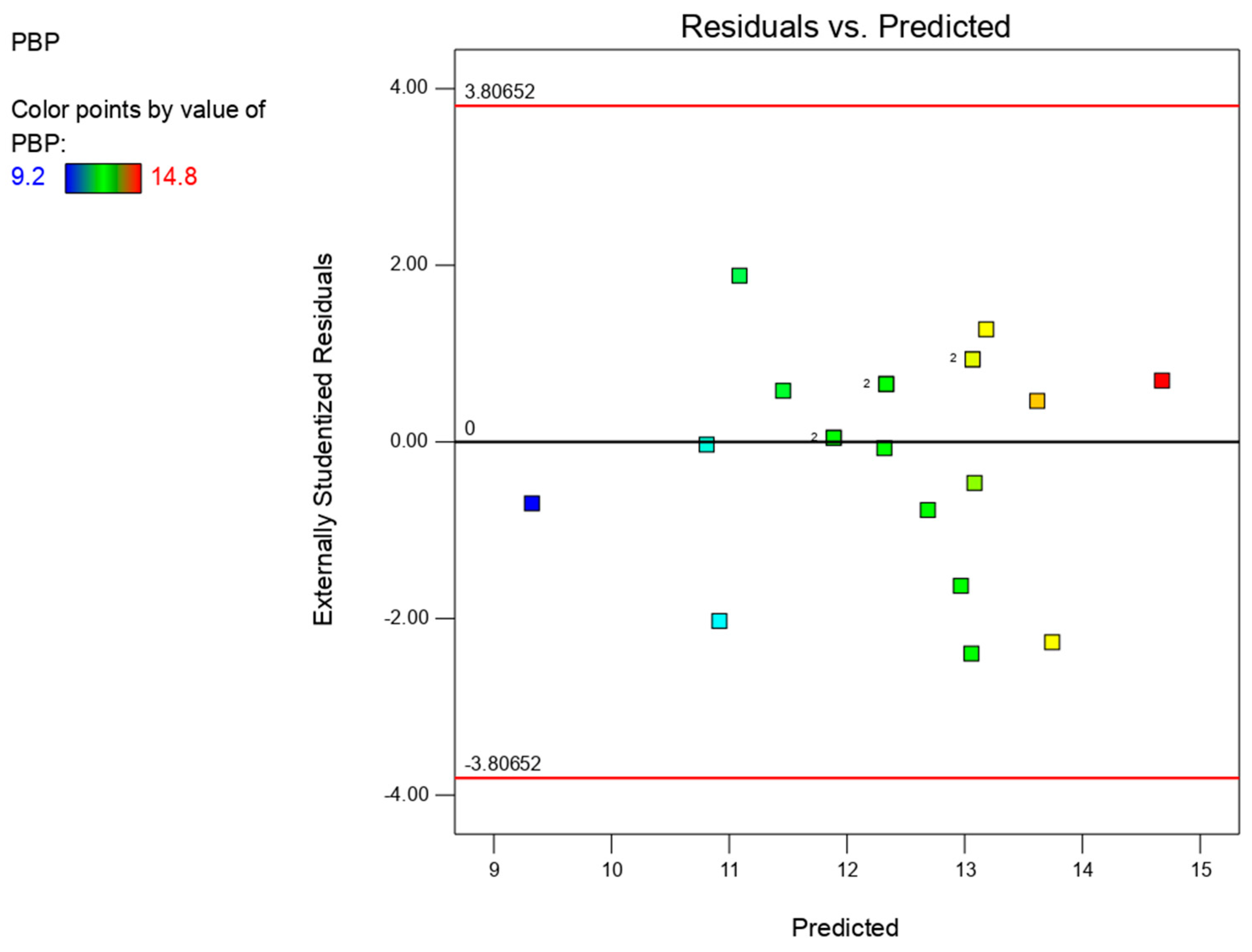
Residuals account for the difference between observed and fitted values predicted by a regression model and verify the model’s sufficiency. Smaller residuals correlate to more accurate regression models. Figure 6 and Figure 7 are plots of the normal probability of the residuals and the residuals versus the predicted response. The normality assumption states that the mean sampling distribution is normal. A check on Figure 6 displays that the residual values generally fall on a straight line, implying that residuals of the response value are distributed normally. In other words, the normal assumption is fulfilled.
The assumption of the independence of errors means there is no relationship between the residuals of our model and the response variable (PBP). In the residuals versus predicted plot, Figure 7, the residuals seem randomly scattered, and the correlation is around zero. Therefore, this assumption is satisfied. The homogeneity of variance assumption states that independent groups must have the same or similar variance. Figure 7 indicates no apparent pattern or unusual structure, which means that the residues are randomly distributed. The residual analysis suggests no reason to suspect any violation of the constant variance or independence assumption. Consequently, the proposed model is sufficient to explore the design space.

6.2.2. Response Surface Analysis

Three-dimensional and their corresponding contour plots based on the regression model were generated to illustrate how the factors affect the PBP. These curves can represent the interaction between the combinations of factors, visually revealing their influence on the PBP response. Drawing on the statistical analysis results that point out the influence of electrical energy purchasing cost, the size of the PV plant, and the interaction of both factors on the PBP, the response surface analysis focuses on the regression surface generated by both independent variables.
Figure 8 illustrates the three-dimensional surface adjacent to their two-dimensional estimated contour plots of the combined effect of PV plant size (A) and electrical energy purchasing cost (C) on the PBP at a PEM capital cost reduction (B) of (a) 0%, (b) 20%, and (c) 40%. The interaction term means that the regression surface is not flat but represents a bend that, in this case, accentuates the reduction in the PBP as the PV plant size and the purchase cost of electricity decrease. Likewise, the minor influence of the reduction in PEM capital cost is confirmed by showing that when it varies from 0% (Figure 8a) to 20% (Figure 8b) and finally to 40% (Figure 8c), the regression surface displaces slightly along the PBP axis, without altering the surface form substantially. PEM reductions above 14.4% already generate PBP values equal to 10 years at electrical energy purchasing costs of USD 0.1150 per kWh and a PV plant size of 200 kW. When the maximum reduction in PEM capital cost is reached (Figure 8c), values equal to or less than 10 years of PBP are generated from values lower than USD 0.12146 per kWh and 280 kW. The plots reveal that both factors have considerable influence on the PBP but that only in a reduced region of the design space are values found that meet the threshold of 10 years for plant economic viability.

6.2.3. Optimum Condition

Desirability functions are a method to optimize models. Optimization objectives may be set to minimize, maximize, or obtain the response’s target value. Desirability function values lie between 0 and 1. A value of 0 indicates that the factors provide an undesirable response, while 1 indicates that they perform optimally. The desirability function plots of this model are given in Figure 9. The desirability of 0.961 is achieved at a 200 kW PV plant size, a reduction in the PEM capital cost of 40%, and USD 0.115 per kWh of electrical energy purchasing cost, resulting in a PBP of 9.4 years (Figure 9c).

7. Study Limitations

The investment performance measurement that evaluates the economic viability of the proposed design is the simple payback period (PBP). Businesses that tend to make relatively small investments and have constant cash flows will find the PBP particularly useful. However, the payback period has two drawbacks: (1) the net cash inflows are not adjusted for the time value of money, and (2) it does not assess cash flows after the payback period. Considering the time value of money, early cash flows received by a project get a better weighting than later cash flows. Additionally, the most significant cash flows may not materialize until after the payback period has finished for some projects. Consequently, their returns on investment may be higher than those from projects with shorter payback times. In these instances, the payback method could dismiss profitable configurations that generate higher cash flows outside the threshold of 10 years. The first deficiency may be remedied by discounting future cash flows and recognizing the time value of money. Nevertheless, our primary concern is assessing how the significant factors affect the system’s economic viability, achieved even without regard to a discount rate. Another shortcoming stems from the input data not considered for the economic evaluation, such as interest rate, inflation, and taxation. These parameters could further diminish the design space where projects are economically viable. Even though including these parameters would provide a more precise mapping of the design space, we have omitted them to simplify our analysis.

8. Conclusions

This study investigated the economic viability at the pre-feasibility level and on a small-scale plant producing methanol and methane based on biogas coupled to a PV power plant and a PEM electrolyzer using the Response Surface Methodology approach. Given that the aim was to provide clean fuels for the cooking sector in Uganda and due to scarce information on costs and the implementation of these fuels, fuel sales prices were assumed as equivalent to the price of LPG cooking gas. First, a preliminary analysis of the reference case was conducted to identify the components’ costs that most impact the plant’s economic viability. This reference case consisted of a 25 Nm3/h anaerobic digestor undergoing cleaning and upgrading to produce methane and a 140 kW PEM electrolyzer-based methanol plant powered by a 200 kW PV plant and grid power. Based on this configuration and electricity price of USD 0.1150 per KWh, the PBP obtained was higher than the threshold of 10 years of PBP for plant economic viability. Later, sensitivity analysis with the RSM approach led to assessing the influence of the three main design variables—PV plant size, electrical energy purchasing cost, and reduction in PEM capital cost—on the PBP response.
Around 750 households in Uganda could be supplied throughout the year with 33.3 tons of methanol and 70.1 tons of biomethane. The PV power plant and the PEM electrolyzer are the most influential components in capital costs, representing 50% and 25%, respectively. Meanwhile, the biogas upgrading, anaerobic digestor, and methanol synthesis units resulted in a marginal value, representing 25% of the total cost. Due to its impact on capital cost and importance in ensuring the plant’s continued operation, the size of the PV plant was a factor to be considered in the sensitivity analysis. Given the close dependence between PV plant size and energy purchased from the grid to meet the proposed plant’s energy demand, the electricity price variation was part of the sensitivity analysis. In addition, PEM electrolyzer capital costs and their potential reduction were also important considerations for its inclusion.
The effect of PV plant size was the most considerable factor associated with the PBP response, followed by electrical energy purchasing cost, the interaction between both factors, and finally, the PEM electrolyzer capital cost reduction. These findings point to energy generation costs as the major factor impacting the economic viability of these small-scale designs, even more than the PEM’s capital cost reduction variable. The response surface analysis revealed that only in a reduced region of the design space are values found that meet the threshold of 10 years for plant economic viability. Specifically, values equal to or less than 10 years of PBP are generated from PEM reductions above 14.4% at electrical energy purchasing costs of USD 0.1150 per kWh and a PV plant size of 200 kW maximum, a reduction in PEM capital cost of 40%, and values lower than USD 0.1215 per kWh and 280 kW. The minimum PBP value of 9.4 years can be obtained in an optimal combination of factors.
Research on small-scale decentralized methanol and methane production based on biogas has uncovered economic viability, albeit in a small region of the design space. Towards this end, advancing the modularity and flexibility of the proposed plant components could, in the future, provide benefits of generating clean biogas-based fuels for upgrading or transforming into synthetic fuels that are accessible to populations in LMICs.

Author Contributions

Funding acquisition, R.B.; Investigation, R.B. and R.Z.B.; Methodology, R.Z.B.; Software, R.Z.B.; Writing—original draft, R.B. and R.Z.B.; Writing—review and editing, R.B. and R.Z.B. All authors have read and agreed to the published version of the manuscript.

Funding

This research was funded by the German Federal Ministry of Education and Research (BMBF) through its Project Management Agency Jülich (PtJ) under the framework of RETO-DOSSO Project with grant No 03SF0598A. The APC was funded by the same.

Data Availability Statement

The data presented in this study are available in Section 4, Section 5 and Section 6.

Acknowledgments

The authors would like to acknowledge the German Federal Ministry of Education and Research (BMBF) for funding this research under the framework of the RETO-DOSSO project.

Conflicts of Interest

The authors declare no conflict of interest.

References

  1. World Health Organization. WHO Guidelines for Indoor Air Quality: Household Fuel Combustion. 2014. Available online: https://www.who.int/publications/i/item/9789241548885 (accessed on 14 March 2022).
  2. Energy Sector Management Assistance Program. What Drives the Transition to Modern Energy Cooking Services? A Systematic Review of the Evidence; World Bank: Washington, DC, USA, 2021; Available online: https://openknowledge.worldbank.org/handle/10986/35199 (accessed on 22 March 2022).
  3. Quinn, A.K.; Bruce, N.; Puzzolo, E.; Dickinson, K.; Sturke, R.; Jack, D.W.; Mehta, S.; Shankar, A.; Sherr, K.; Rosenthal, J.P. An analysis of efforts to scale up clean household energy for cooking around the world. Energy Sustain. Dev. 2018, 46, 1–10. [Google Scholar] [CrossRef] [PubMed]
  4. Putti, V.R.; Michael, T.; Mehta, S.; Kammila, S. The State of the Global Clean and Improved Cooking Sector; World Bank: Washington, DC, USA, 2015; Available online: https://openknowledge.worldbank.org/bitstream/handle/10986/21878/96499.pdf?sequence=1&isAllowed=y (accessed on 5 April 2022).
  5. Lwiza, F.; Mugisha, J.; Walekhwa, P.N.; Smith, J.; Balana, B. Dis-adoption of Household Biogas technologies in Central Uganda. Energy Sustain. Dev. 2017, 37, 124–132. [Google Scholar] [CrossRef] [Green Version]
  6. Lutaaya, F. Quality and Usage of Biogas Digesters in Uganda. Master’s Thesis, Royal Institute of Technology, Stockholm, Sweden, 2013. Available online: https://www.diva-portal.org/smash/get/diva2:661963/FULLTEXT01.pdf (accessed on 7 July 2022).
  7. Clemens, H.; Bailis, R.; Nyambane, A.; Ndung’u, V. Africa Biogas Partnership Program: A review of clean cooking implementation through market development in East Africa. Energy Sustain. Dev. 2018, 46, 23–31. [Google Scholar] [CrossRef] [PubMed]
  8. Figueroa, A.; Boshell, F.; van Velzen, L.; Anisie, A. Biogas for Domestic Cooking: Technology Brief; IRENA: Abu Dhabi, United Arab Emirates, 2017; Available online: https://www.irena.org/publications/2017/Dec/Biogas-for-domestic-cooking-Technology-brief (accessed on 19 August 2022).
  9. Puzzolo, E.; Pope, D.; Stanistreet, D.; Rehfuess, E.A.; Bruce, N.G. Clean fuels for resource-poor settings: A systematic review of barriers and enablers to adoption and sustained use. Environ. Res. 2016, 146, 218–234. [Google Scholar] [CrossRef] [PubMed]
  10. Vijay, V.K.; Kapoor, R.; Trivedi, A.; Vijay, V. Biogas as Clean Fuel for Cooking and Transportation Needs in India. In Advances in Bioprocess Technology; Ravindra, P., Ed.; Springer International Publishing: Cham, Switzerland, 2015; pp. 257–275. [Google Scholar] [CrossRef]
  11. Ozier, A.; Charron, D.; Chung, S.; Sarma, V.; Dutta, A.; Jagoe, K.; Obueh, J.; Stokes, H.; Munangagwa, C.L.; Johnson, M.; et al. Building a consumer market for ethanol-methanol cooking fuel in Lagos, Nigeria. Energy Sustain. Dev. 2018, 46, 65–70. [Google Scholar] [CrossRef] [PubMed]
  12. Moioli, E.; Wötzel, A.; Schildhauer, T. Feasibility assessment of small-scale methanol production via power-to-X. J. Clean Prod. 2022, 359, 132071. [Google Scholar] [CrossRef]
  13. Topriska, E.; Kolokotroni, M.; Dehouche, Z.; Wilson, E. Solar hydrogen system for cooking applications: Experimental and numerical study. Renew. Energy 2015, 83, 717–728. [Google Scholar] [CrossRef] [Green Version]
  14. Topriska, E.; Kolokotroni, M.; Dehouche, Z.; Novieto, D.T.; Wilson, E.A. The potential to generate solar hydrogen for cooking applications: Case studies of Ghana, Jamaica and Indonesia. Renew. Energy 2016, 95, 495–509. [Google Scholar] [CrossRef]
  15. Onwe, C.A.; Rodley, D.; Reynolds, S. Modelling and simulation tool for off-grid PV-hydrogen energy system. Int. J. Sustain. Energy 2020, 39, 1–20. [Google Scholar] [CrossRef]
  16. Rivera, X.C.S.; Topriska, E.; Kolokotroni, M.; Azapagic, A. Environmental sustainability of renewable hydrogen in comparison with conventional cooking fuels. J. Clean Prod. 2018, 196, 863–879. [Google Scholar] [CrossRef]
  17. Owusu, P.A.; Banadda, N. Livestock waste-to-bioenergy generation potential in Uganda. Environ. Res. Eng. Manag. 2017, 73, 45–53. [Google Scholar] [CrossRef] [Green Version]
  18. Okello, C.; Pindozzi, S.; Faugno, S.; Boccia, L. Bioenergy potential of agricultural and forest residues in Uganda. Biomass Bioenergy 2013, 56, 515–525. [Google Scholar] [CrossRef]
  19. World Health Organization. WHO Air Quality Guidelines Global Update 2005: Particulate Matter, Ozone, Nitrogen Dioxide and Sulfur Dioxide; World Health Organization: Copenhagen, Denmark, 2006; Available online: https://www.euro.who.int/__data/assets/pdf_file/0005/78638/E90038.pdf (accessed on 18 March 2022).
  20. World Health Organization. WHO Guidelines for Indoor Air Quality: Selected Pollutants; World Health Organization: Bonn, Germany, 2010; Available online: https://www.euro.who.int/__data/assets/pdf_file/0009/128169/e94535.pdf (accessed on 18 March 2022).
  21. Rehfuess, E.; Pope, D.; Bruce, N.; Dherani, M.; Jagoe, K.; Naeher, L.; Noonan, C. WHO Indoor Air Quality Guidelines: Household Fuel Combustion—Review 6: Impacts of interventions on PM and CO; WHO: Geneva, Switzerland, 2014. [Google Scholar]
  22. Pope, D.; Bruce, N.; Dherani, M.; Jagoe, K.; Rehfuess, E. Real-life effectiveness of ‘improved’ stoves and clean fuels in reducing PM2.5 and CO: Systematic review and meta-analysis. Environ. Int. 2017, 101, 7–18. [Google Scholar] [CrossRef] [PubMed]
  23. Pope, D.; Johnson, M.; Fleeman, N.; Jagoe, K.; Duarte, R.; Maden, M.; Ludolph, R.; Bruce, N.; Shupler, M.; Adair-Rohani, H.; et al. Are cleaner cooking solutions clean enough? A systematic review and meta-analysis of particulate and carbon monoxide concentrations and exposures. Environ. Res. Lett. 2021, 16, 83002. [Google Scholar] [CrossRef]
  24. Bates, M.N.; Bruce, N.; Lam, N.L.; Smith, K.R.; Gauthier, A. WHO Indoor Air Quality Guidelines: Household Fuel Combustion—Review 9: Summary of systematic review of household kerosene use. J. Toxicol. Environ. Health B Crit. Rev. 2021, 15, 396–432. [Google Scholar]
  25. Lam, N.L.; Smith, K.R.; Gauthier, A.; Bates, M.N. Kerosene: A review of household uses and their hazards in low-and middle-income countries. J. Toxicol. Environ. Health Part B Crit. Rev. 2012, 15, 396–432. [Google Scholar] [CrossRef] [Green Version]
  26. Hoefsloot, H.C.J.; Vis, D.J.; Westerhuis, J.A.; Smilde, A.K.; Jansen, J.J. Multiset Data Analysis: ANOVA Simultaneous Component Analysis and Related Methods. Compr. Chemom. 2009, 2, 453–472. [Google Scholar] [CrossRef]
  27. Sarabia, L.A.; Ortiz, M.C. Response Surface Methodology. Compr. Chemom. 2009, 1, 345–390. [Google Scholar]
  28. Jankovic, A.; Chaudhary, G.; Goia, F. Designing the design of experiments (DOE)—An investigation on the influence of different factorial designs on the characterization of complex systems. Energy Build 2021, 250, 111298. [Google Scholar] [CrossRef]
  29. Box, G.E.P.; Wilson, K.B. On the Experimental Attainment of Optimum Conditions. J. R. Stat. Soc. Ser. B 1951, 13, 1–45. Available online: https://www.jstor.org/stable/2983966 (accessed on 14 September 2022). [CrossRef]
  30. Cochran, W.G.; Cox, G.M. Experimental Designs, 2nd ed.; John Wiley & Sons: New York, NY, USA, 1957. [Google Scholar]
  31. Box, G.E.P.; Hunter, J.S. Multi-Factor Experimental Designs for Exploring Response Surfaces. Ann. Math. Stat. 1957, 28, 195–241. Available online: https://www.jstor.org/stable/2237033 (accessed on 25 August 2022). [CrossRef]
  32. Hurtubia, B.; Sauma, E. Economic and environmental analysis of hydrogen production when complementing renewable energy generation with grid electricity. Appl. Energy 2021, 304, 117739. [Google Scholar] [CrossRef]
  33. Holst, M.; Aschbrenner, S.; Smolinka, T.; Voglstätter, C.; Grimm, G. Cost Forecast for Low Temperature Electrolysis—Technology Driven Bottom-up Prognosis for PEM and Alkaline Water Electrolysis Systems; Fraunhofer Institute for Solar Energy Systems ISE: Freiburg, Germany, 2021; Available online: https://www.ise.fraunhofer.de/content/dam/ise/de/documents/publications/studies/cost-forecast-for-low-temperature-electrolysis.pdf (accessed on 7 September 2022).
  34. Kannah, R.Y.; Kavitha, S.; Preethi; Karthikeyan, O.P.; Kumar, G.; Dai-Viet, N.V.; Banu, J.R. Techno-economic assessment of various hydrogen production methods—A review. Bioresour. Technol. 2020, 319, 124175. [Google Scholar] [CrossRef] [PubMed]
  35. Black, M.J.; Roy, A.; Twinomunuji, E.; Kemausuor, F.; Oduro, R.; Leach, M.; Sadhukhan, J.; Murphy, R. Bottled biogas—An opportunity for clean cooking in Ghana and Uganda. Energies 2021, 14, 14. [Google Scholar] [CrossRef]
  36. Nock, W.J.; Walker, M.; Kapoor, R.; Heaven, S. Modeling the water scrubbing process and energy requirements for CO2 capture to upgrade biogas to biomethane. Ind. Eng. Chem. Res. 2014, 53, 12783–12792. [Google Scholar] [CrossRef] [Green Version]
  37. Bekkering, J.; Broekhuis, A.A.; van Gemert, W.J.T. Optimisation of a green gas supply chain—A review. Bioresour. Technol. 2010, 101, 450–456. [Google Scholar] [CrossRef]
  38. Sun, Q.; Li, H.; Yan, J.; Liu, L.; Yu, Z.; Yu, X. Selection of appropriate biogas upgrading technology-a review of biogas cleaning, upgrading and utilization. Renew. Sustain. Energy Rev. 2015, 51, 521–532. [Google Scholar] [CrossRef]
  39. Twinomunuji, E.; Kemausuor, F.; Black, M.; Roy, A.; Leach, M.; Sadhukhan, R.O.J.; Murphy, R. The Potential for Bottled Biogas for Clean Cooking in Africa; Modern Energy Cooking Services. 2020. Available online: https://www.mecs.org.uk/wp-content/uploads/2020/12/Potential-for-bottled-biogas-for-clean-cooking-in-Africa_Feb-2020-working-paper.pdf (accessed on 20 July 2022).
  40. Ushikoshi, K.; Mori, K.; Watanabe, T.; Takeuchi, M. A 50 kg/day class test plant for methanol synthesis from CO2 and H2. Adv. Chem. Convers. Mittigating Carbon Dioxide 1998, 114, 357–362. [Google Scholar]
  41. Schemme, S.; Breuer, J.L.; Koller, M.; Meschede, S.; Walman, F.; Samsun, R.C.; Peters, R.; Stolten, D. H2-based synthetic fuels: A techno-economic comparison of alcohol, ether and hydrocarbon production. Int. J. Hydrog. Energy 2020, 45, 5395–5414. [Google Scholar] [CrossRef]
  42. Korpås, M.; Greiner, C.J. Opportunities for hydrogen production in connection with wind power in weak grids. Renew Energy 2008, 33, 1199–1208. [Google Scholar] [CrossRef]
  43. Aarakit, S.M.; Ssennono, V.F.; Adaramola, M.S. Estimating Market Potential for Solar Photovoltaic Systems in Uganda. Front. Energy Res. 2021, 9, 602468. [Google Scholar] [CrossRef]
  44. Oloya, I.T.; Gutu, T.J.L.; Adaramola, M.S. Techno-economic assessment of 10 MW centralised grid-tied solar photovoltaic system in Uganda. Case Stud. Therm. Eng. 2020, 25, 100928. [Google Scholar] [CrossRef]
  45. Electricity Regulatory Authority. Electricity Tariff Schedules in Uganda. Electricity Regulatory Authority. 2022. Available online: https://www.era.go.ug/index.php/tariffs/tariff-schedules (accessed on 7 June 2022).
  46. Garland, C.; Jagoe, K.; Wasirwa, E.; Nguyen, R.; Roth, C.; Patel, A.; Shah, N.; Derby, E.; Mitchell, J.; Pennise, D.; et al. Impacts of household energy programs on fuel consumption in Benin, Uganda, and India. Energy Sustain. Dev. 2015, 27, 168–173. [Google Scholar] [CrossRef]
  47. Price, R. ‘Clean’ Cooking Energy in Uganda—Technologies, Impacts, and Key Barriers and Enablers to Market Acceleration; K4D Helpdesk Report; Institute of Development Studies: Brighton, UK, 2017; p. 2. [Google Scholar]
  48. Bruce, N.G.; Aunan, K.; Rehfuess, E.A. Liquefied Petroleum Gas as a Clean Cooking Fuel for Developing Countries: Implications for Climate, Forests, and Affordability. 2017. Available online: https://www.kfw-entwicklungsbank.de/PDF/Download-Center/Materialien/2017_Nr.7_CleanCooking_Lang.pdf (accessed on 20 April 2022).
  49. Amigun, B.; von Blottnitz, H. Capital cost prediction for biogas installations in Africa: Lang factor approach. Environ. Prog. Sustain. Energy 2009, 28, 134–142. [Google Scholar] [CrossRef]
  50. Guthrie, K.M. Data and Techniques for Preliminary Capital Cost Estimating; McGraw-Hill: New York, NY, USA, 1969; pp. 114–142. [Google Scholar]
  51. Ulrich, G.D. A Guide to Chemical Engineering Process Design and Economics; John Wiley and Sons: New York, NY, USA, 1984. [Google Scholar]
  52. International Energy Agency. Capital Costs of Utility-Scale Solar PV in Selected Emerging Economies. 2020. Available online: https://www.iea.org/data-and-statistics/charts/capital-costs-of-utility-scale-solar-pv-in-selected-emerging-economies (accessed on 23 September 2022).
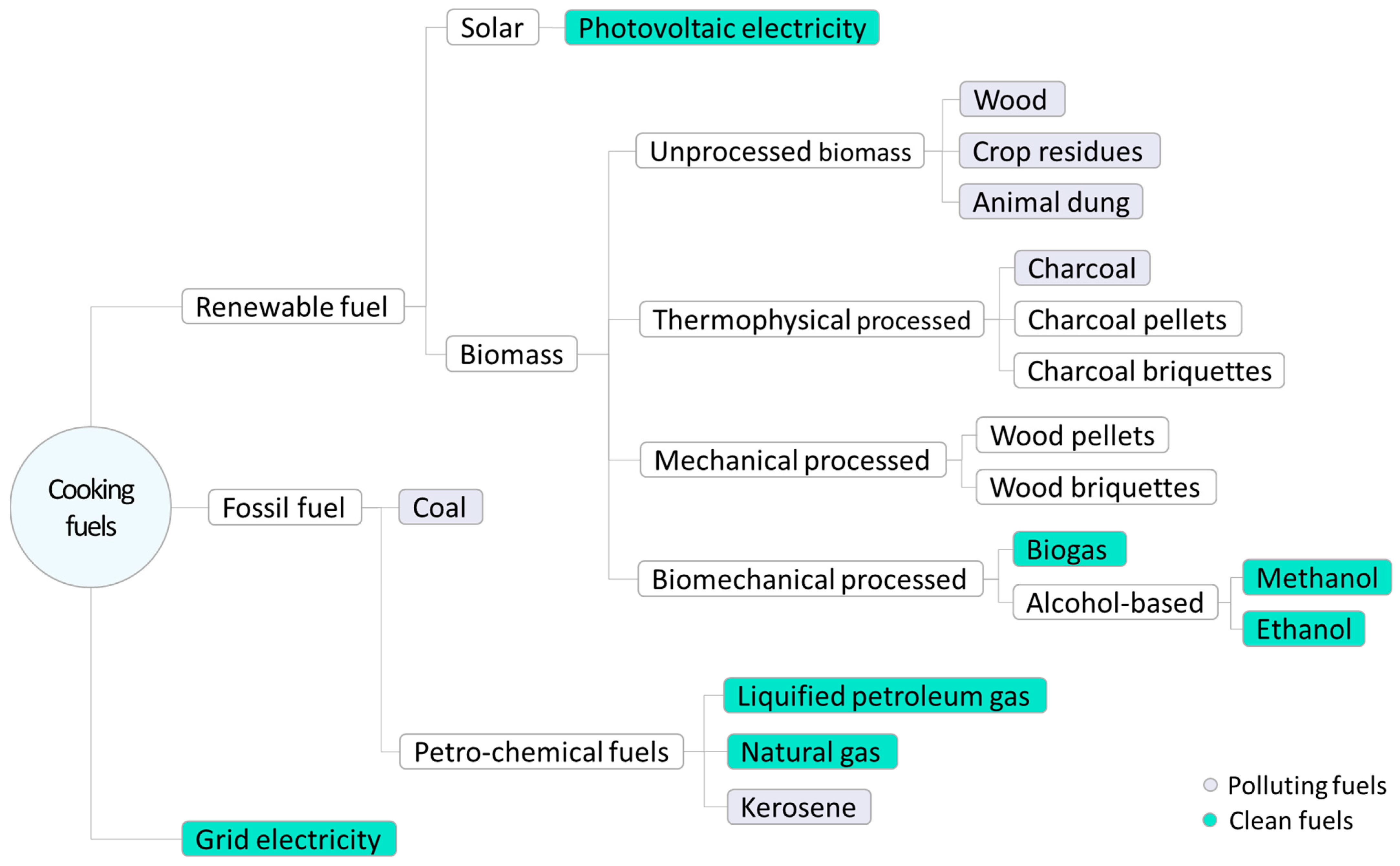
Figure 1. Classification of cooking fuels as clean or polluting at the point of use.
Energies 15 09329 g001
Figure 2. Three-factor response surface designs: (a) Two-level full factorial, (b) Three-level full factorial, (c) Face-Centered Central Composite, and (d) Box–Behnken designs. Blue dots: factorial, red dots: center, green dots: edge, yellow dots: axial (star).
Energies 15 09329 g002
Figure 3. Layout of the hybrid methanol–methane production plant.
Energies 15 09329 g003
Figure 4. Breakdown and percentage distribution of the purchased equipment cost of the hybrid methanol–methane production plant.
Energies 15 09329 g004
Figure 5. PBP—perturbation factors plot at the design space’s midpoint.
Energies 15 09329 g005
Figure 6. Plot of normal probability of residuals for PBP data.
Energies 15 09329 g006
Figure 7. Plot of residuals vs. predicted PBP response data.
Energies 15 09329 g007
Figure 8. Response surface and contour plots for PV plant size and electrical energy purchasing cost on the PBP at a reduction in PEM capital cost of (a) 0%, (b) 20%, and (c) 40%.
Energies 15 09329 g008
Figure 9. Desirability function plots. (a) Response surface plot of overall desirability function. (b) PBP response surface plot associated with the desirability function. (c) Desirability ramp for achieving optimum PBP.
Energies 15 09329 g009
Table 1. Specification of Engas UK’s 25 Nm3/h bio-CNG upgrader. Source: Black et al., (2021) [35] and Twinomunuji et al. (2020) [39].
ParametersSpecifications
Raw biogas flow rate25 Nm3/h
Raw biogas specification50–65% CH4; 50–35% CO2; 500 ppm H2S
Inlet biogas pressure7–20 mbar
Outlet methane gas pressure3–5 bar
Outlet methane gas pressure after compression250 bar
Outlet methane specification2% CO2; 97–98% CH4; 5 mg/m3 H2S
Upgrading and compression energy consumption 0.5 kWh/Nm3 of raw biogas
Water consumption with regeneration2 L of water/ Nm3 of raw biogas
Table 2. Technical parameters of the sub-systems.
Sub-SystemParameter
Anaerobic digestionRaw biogas output flow rate: 25 Nm3/h
Chemical composition of biogas [6]: 54% CH4 and 46% CO2
Biogas cleaning and upgradingCH4 losses [37]: 2%
CO2 losses [38]: 20%
Electricity consumption [39]: 0.5 kWh/Nm3 raw biogas
Methanol synthesis unitStoichiometric H2: CO2 ratio: 3:1
Working Pressure: 50 bar
Temperature: 250 °C
Conversion efficiency: 96%
Electrical energy demand: 0.154 kWh/kg of methanol [41]
PEM water electrolyzerSpecific power consumption: 56.7 kWh/kg [13]
Photovoltaic power plantPerformance ratio: 75.84%, [44]
Daily solar radiation [44]:
Minimum: 5.22 kWh/m2/day
Average: 5.85 kWh/m2/day
Maximum: 6.28 kWh/m2/day
Table 3. Methods and references for cost estimation of the main components of the hybrid methanol–methane plant.
Sub-SystemMethod/Reference
Anaerobic digesterRetrieved from Black et al. (2021) [35]
Biogas upgrading and compressionRetrieved from Black et al. (2021) [35]
Methanol synthesis unitBare module cost as a function of the equipment type ( C p ), material ( F M ), volume, and pressure ( F P ) [50,51]:
C B M = f ( C p , F M , F P )
The material considered is stainless steel and the cost is actualized to current price through the Chemical Engineering Plant Cost Index (CEPCI)
PEM water electrolyzerBased on the estimates of Holst et al. (2021)
Photovoltaic power plantBased on the estimates of the International Energy Agency International Energy Agency [52]
Table 4. Summary of thermodynamic results: annual mass and energy balance.
ParameterValueUnit
PV plant production323.9MWh/year
Electrical energy purchased from the grid892.7MWh/year
Electrical energy consumption1216.5MWh/year
Methanol production33.3ton/year
Biomethane production70.1ton/year
Oxygen production155.8ton/year
Table 5. Summary of annual cash inflow.
Annual Revenue
Methane incomeUSD 172,821
Methanol incomeUSD 38,861
Oxygen incomeUSD 20,254
Sub-totalUSD 231,936
Annual costs
Variable costsUSD 102,656
Sub-totalUSD 102,656
Annual cash inflow
TotalUSD 129,279
Table 6. Dependent variables and levels for the Face-Centered Central Composite design.
FactorNameUnitValues of Coded Levels
−101
APV plant sizekW200450700
BPercentage reduction in PEM capital cost%02040
CElectricity priceUSD/kWh0.1150.1320.149
Table 7. Design matrix and results of the Face-Centered Central Composite design.
RunBlockFactorsResponse
PV Plant Size (kW)Percentage Reduction in PEM Capital Cost (%)Electricity Price (USD/kWh)Payback Period
(Years)
1170000.14914.8
21450200.13213.3
31700400.11513.7
4120000.11510.6
51200400.14912.7
61450200.13213.3
72450200.13212.5
8220000.14913.4
92700400.14913.0
102450200.13212.5
11270000.11513.4
122200400.1159.2
133450200.13211.9
143450400.13211.6
153450200.11511.5
163700200.13212.6
17345000.13212.3
183200200.13210.8
193450200.13211.9
203450200.14912.5
Table 8. Model summary statistics.
SourceStd. Dev.Adjusted R²Predicted R²PRESSSequential p-Value
Linear0.59050.80310.76090.348516.15<0.0001
2FI0.24720.97290.95810.73036.69<0.0001
Quadratic0.20570.98630.9710.75496.080.1218
Table 9. ANOVA for the 2FI model.
SourceSum of Squares Degree of Freedom Mean SquareF-Valuep-ValueContribution
Block4.7822.39
Model24.1264.0265.77<0.0001
A-PV plant size11.66111.66190.81<0.000148.34%
B-Reduction in PEM capital cost1.8511.8530.250.00027.67%
C-Electrical energy purchasing cost6.416.4104.7<0.000126.53%
AB0.04510.0450.73620.40920.19%
AC3.9213.9264.13<0.000116.25%
BC0.24510.2454.010.07061.02%
Residual0.6724110.0611
Cor Total29.5819
Table 10. Fit statistics.
Statistical ParameterValue
R20.9612
Adjusted R20.9492
Predicted R20.8606
Adeq Precision33.2568
Std. Dev.0.2721
Mean12.38
C.V.%2.2
Table 11. ANOVA for the reduced 2FI model.
SourceSum of Squares Degree of Freedom Mean SquareF-Valuep-ValueContribution
Block4.7822.39
Model23.8345.9680.48<0.0001
A-PV plant size11.66111.66157.55<0.000148.93%
B-Reduction in PEM capital cost1.8511.8524.980.00027.76%
C-Electrical energy purchasing cost6.416.486.45<0.000126.86%
AC3.9213.9252.95<0.000116.45%
Residual0.9624130.074
Cor Total29.5819
Publisher’s Note: MDPI stays neutral with regard to jurisdictional claims in published maps and institutional affiliations.