Trajectory Clustering and k-NN for Robust Privacy Preserving k-NN Query Processing in GeoSpark

Abstract

Privacy Preserving and Anonymity have gained significant concern from the big data perspective. We have the view that the forthcoming frameworks and theories will establish several solutions for privacy protection. The k-anonymity is considered a key solution that has been widely employed to prevent data re-identifcation and concerns us in the context of this work. Data modeling has also gained significant attention from the big data perspective. It is believed that the advancing distributed environments will provide users with several solutions for efficient spatio-temporal data management. GeoSpark will be utilized in the current work as it is a key solution that has been widely employed for spatial data. Specifically, it works on the top of Apache Spark, the main framework leveraged from the research community and organizations for big data transformation, processing and visualization. To this end, we focused on trajectory data representation so as to be applicable to the GeoSpark environment, and a GeoSpark-based approach is designed for the efficient management of real spatio-temporal data. Th next step is to gain deeper understanding of the data through the application of k nearest neighbor (k-NN) queries either using indexing methods or otherwise. The k-anonymity set computation, which is the main component for privacy preservation evaluation and the main issue of our previous works, is evaluated in the GeoSpark environment. More to the point, the focus here is on the time cost of k-anonymity set computation along with vulnerability measurement. The extracted results are presented into tables and figures for visual inspection.

1. Introduction

There is no doubt that we live in the era of Big Data. Over the last decade, thanks to technological advances, information systems have favored automatic and effective data gathering, thus resulting in a considerable increase in the amount of available data. Daily, a wide range of data is produced: scientific, financial, health data, as well as from social media, are just some examples of sources. However, this data is useless without the extraction of the underlying knowledge, a major challenge for the researchers as classical machine learning methods cannot deal with the volume, value, veracity and variety that big data brings [1]. Therefore, existing machine learning techniques, which deal with 4 Vs [2], have been or need to be redefined for efficiently processing and managing such data, as well as to obtain valuable information that can benefit not only scientists, but also businesses and organizations. Actually, the recent advances in distributed technologies can be utilized in order to enable scientists to rapidly find out hidden or unknown patterns from the 4 Vs [3]. Nonetheless, most of the existing methods fail to directly tackle the increased number of attributes and records of databases, due to its computational complexity. Hence, the data mining techniques should be able to encounter data scalability, dimensionality, uncertain data and/or data preprocessing. Data preprocessing constitutes an important step before the data mining process and, as a result, data mining algorithms are designed to accept specific data formats that are best suited for them.

With the advances in wireless and mobile technologies, moving objects are equipped with location positioning sensors and wireless communicating capabilities, thus, large-scale spatio-temporal data is being generated and an urgent need for efficient query processing approaches, to deal with both the spatial and temporal attributes, has been arisen [4]. In particular, with the advent of mobile and ubiquitous computing, spatio-temporal queries processing on moving objects databases has become a necessity for many applications, such as traffic control systems, geographical information systems, and location-aware advertisement. Hence, time-dependent versions of k nearest neighbor (k-NN) queries need to be studied. According to [5], the k-NN queries can be distinguished into four categories: (i) both query and data objects are static, (ii) moving query but static data objects, (iii) static query but moving data objects and (iv) both query and data objects are moving. When a mobile object’s location data changes, a Snapshot k-NN ($SkNN$) query is issued at each location. However, in highly dynamic spatio-temporal applications, where the moving objects data varies frequently over time, a fundamental query is the so-called Continuous k-NN ($CkNN$) [6]. A $CkNN$ query can be subjected to the fourth category, as it instantly retrieves the k nearest neighbor objects of a moving query object at each time within a given time interval. Practically, the $CkNN$ spatio-temporal query is evaluated on a high number of consecutive timestamps and can be considered as a series of frequent $SkNN$ queries. To the best of our knowledge, none of the existing approaches, such as [6,7,8] to name a few, address the problem of $CkNN$ queries processing on non-linear trajectories under the support of Hough transformation. It is worth to mention that in previous works the process of $CkNN$ query has been considered in road networks with linear trajectory moving objects.

In this paper, our efforts are devoted to processing a $CkNN$ query assuming that each object keeps track of non-linear trajectory. Such a trajectory is approximated as piece-wise linear among timestamps where objects (small) velocity changes; a storage efficient strategy adopted in our previous work [9]. Some previous works investigate the problem of $CkNN$ for moving objects with fixed velocity while others with uncertain velocity in road networks [10,11]. Nonetheless, once an object’s velocity changes, the $CkNN$ query has to be re-executed. Such a case is quite frequent in highly dynamic environments, thus, the performance of these techniques would be significantly degraded, resulting in increased query cost (because of re-evaluation). The focus of this work is on k nearest neighbor queries, which are considered under both a spatio-temporal and a Hough transformed database. The Hough method can mitigate such issues since it is piece-wise constant [9], thus, the $CkNN$ query is not evaluated as frequent as in the Euclidean space with non-linear trajectory. Actually, the application of k-NN queries in Hough space facilitates the maintenance and consistency of continuous queries result [12], even if the moving objects location data updates. The aforementioned issue relates to the fact that the query result needs to be only updated upon specific changes, namely, whenever moving angle direction and/or velocity vary dramatically. Nevertheless, while an object (including the query object) is moving on a linear part of its trajectory (maintenance phase) the query result will not change, meaning that the query result of all the objects will not need be revised until the objects transit to the next linear part of its trajectory, which indicates that the maintenance phase expires.

Moreover, with the extensive adoption of the Cloud, research on privacy preserving has appealed to lots of researchers [13,14]. Let us recall that the ultimate purpose of the processing is to formulate the k-anonymity set to protect users’ privacy in the cloud computing environment. Especially, in the context of this work, we are challenged with the necessity to apply temporal continuous spatial k-NN queries in a distributed architecture with the ultimate goal of forming the anonymity set for a group of moving objects in a fast and efficient manner.

In summary, the main contributions of this paper are as follows:

• A continuous query processing algorithm is considered that efficiently answers the spatial k-NN query with the aid of an indexing method or otherwise. From the query result, in each timestamp and for all moving objects, the desired anonymity set is formulated.
• The adopted method is designed with the aid of GeoSpark spatial data operations to compute the k-anonymity set which is used to measure the possibility of each object identity being unveiled as it moves from one location to another. To be more specific, vulnerability evaluation is conducted in two-dimensional space (both Euclidean and Hough space), considering different pairs of features, as it will be demonstrated in Section 4.
• A comprehensive set of experiments is conducted to evaluate the time performance of the proposed method in the GeoSpark environment under different data sizes.

The rest of this paper is organized as follows. In Section 2, previous related works are presented in relation to our approach. In Section 3, the following are described: (a) the problem definition, (b) the system model and (c) the proposed GeoSpark framework for the k-anonymity set computation. Section 4 presents the experiments conducted for the evaluation of the studying problem, while Section 5 evaluates relevant discussion of the studying problem results in relation to previous works. Finally, in Section 6, conclusions and future directions of this work are recorded.

2. Related Work

The domain of efficient management regarding spatio-temporal data has different aspects and extensions which are worth studying, from storage and indexing to time-efficient and robust spatio-temporal queries issuing. It is pointed out here that, in the context of this work, we focus on time efficient privacy preserving spatio-temporal k-NN queries.

2.1. Distributed Frameworks for Spatio-Temporal data Queries Processing

Due to the explosive growth of spatio-temporal data, the domain of distributed execution of spatial queries has gained considerable concern. In [15], a novel framework, known as STARK, is recommended for spatio-temporal data management, which includes spatial partitioners, different modes for indexing, filter, join, and clustering operators. In contrast to existing solutions, STARK is considered an integrated Spark program and provides more flexible and comprehensive operators. Several application scenarios of this framework are presented in [16]. Moreover, the authors in [17] introduce a new abstraction called IndexTRDD to manage trajectory segments, which exploits a global and local indexing mechanism to accelerate trajectory queries. Also, they adaptively update the partition structure based on the change of data distribution to alleviate the partitioning overhead.

In [18], a scalable system for massive trajectory data management is elaborated, which modifies the three core layers of $ST$-Hadoop. Authors in [19] evaluate the distributed execution of spatial SQL queries in GeoSpark and STARK system. Moreover, in order to address the challenges of high velocity location data, authors propose a distributed in-memory spatio-temporal data processing system, which includes a distributed in-memory index and storage infrastructure built on a distributed in-memory programming paradigm [20]. The location records are distributed across a cluster of nodes using the producer–consumer model.

2.2. Efficient Privacy Preserving k-NN Queries

In spatial databases, the processing of k-NN query over stationary objects has be extensively studied. The last decade, thanks to technological advances, real-time spatio-temporal data of moving objects can be monitored and in following processed. Hence, the Continuous k-NN querying in real-time and dynamic environments has attracted the attention of researchers [21]. In [22], the authors attempt to develop an efficient algorithm to process the k-NN queries on uncertain locations of objects. A probability model is designed to quantify the possibility of each object being one of the k nearest neighbors. The uncertainty of the object’s location lies in the fact that their position is monitored by a sensor-based tracking system, instead of the GPS technique.

In a recent work, the authors study the problem of $CkNN$ queries on moving objects to retrieve the k-NNs of all points along a query trajectory in spatial road networks [23]. A novel direction-aware $CkNN$ algorithm, the so-called $DACKNN$, is recommended. To ensure an efficient query, the algorithm excludes from the analysis moving objects that are far away from the query point.

In [24] a fast continuous query privacy-preserving framework in road networks is recommended, based on the concepts of both k-anonymity and l-diversity. The authors in [25] propose a method to make location cloaking less vulnerable to query tracking attacks. The proposed method is applied on road networks, such as subways, railways, and highways, where the road network is known and fixed, except for the trajectories. It is called adaptive-fixed k-anonymization and generates smaller cloaking regions without compromising the privacy of the query issuer’s location.

Futhermore, the authors in [26] study the problem of location disclosure adopting the k-anonymity method in the centralized architecture based on a single trusted anonymizer. However, this strategy may compromise user privacy involving continuous LBSs. A dual-K mechanism (DKM) is suggested to protect the users’ trajectory privacy for continuous LBSs. The proposed method firstly inserted multiple anonymizers between the user and the location service provider (LSP). The k anonymization is achieved by sending k query locations to different anonymizers. To improve user trajectory privacy, the dynamic pseudonym mechanism is combined with the location selection one. Hence, the user trajectory (spatio-temporal points) cannot be obtained by neither the LSP nor the anonymizer.

Note that in our previous work [9], a pseudonyms system is recommended to ensure and/or reinforce the privacy of mobile objects. Actually, a mobile user can initiate a discrete number of k-NN queries in each spatio-temporal point with different pseudonyms for each one. The recommended protocols provide unlinkability, thus, the service provider cannot connect to the IP and validate that they belong to the same user. The main characteristic of this approach is that the k-NN queries can be issued not only in Euclidean space but also in Hough-X/Y space. As the analysis and results show, Hough space is an appropriate solution as it preserves a user’s privacy and provides storage efficiency as well, assuming that the initial non-linear trajectory of a moving object is splitted into a set of linear sub-trajectories.

In this work, the problem of k-anonymity for privacy preserving in spatio-temporal databases is evaluated in a distributed environment. Although traditional privacy preserving solutions have been designed in Euclidean space, our framework assumes the concept of k-anonymity in Hough space as well. Due to the constant evolution of the mobile objects’ location information in time, it is required to evaluate massive single query point k-NN queries for massive mobile objects per timestamp. The spatio-temporal k-NN queries are issued with the aim to formulate the k-anonymity set of moving objects. This set is online computed based on all objects trajectory point in each timestamp and consists of the ids of the k nearest objects. Specifically, in each timestamp, a k-NN query, called Snapshot Trajectory Point k-NN ($STkNN$), is issued taking into consideration the selected features information (e.g., euclidean coordinates, angle and velocity, dual points) of all the objects. Assuming a high time sampling rate, we can claim that the process is similar to a Continuous Trajectory Point k-NN ($CTPkNN$). As we have already mentioned, an important characteristic of continuous k-NN query in Hough space is that the k-NNs in between two consecutive spatio-temporal points remain the same. Based on this characteristic, the problem of performing repetitive queries can be considerably reduced to finding the k-NNs in specific spatio-temporal points where the mobile objects’ velocity varies, indicating a new linear sub-trajectory of the initial non-linear trajectory. Unlike our and other previous works, here, the key idea is to evaluate the proposed method for the k-anonymity set computation in an environment suitable for efficient k-NN query in spatial or dual points data.

3. Materials and Methods

This section provides the necessary background knowledge for the remainder of the paper. Initially, the k-NN algorithm, a core component of the adopted privacy preserving methodology along with its weaknesses to tackle big data problems, is presented. In following, useful definitions and notations will be recorded under the problem definition, with the most characteristic being the spatial indexing and partitioning methods. Moreover, the GeoSpark components for the $CkNN$ queries processing with the aim to formulate the k-anonymity set, will be in detail described.

3.1. Operations on Spatial Data

Querying on spatial data is considered an operation that is usually coupled with indexing methods. Several indexing methods have been considered in literature as they are crucial for the performance of spatial data query processing algorithms, since they are used in order to reduce the query run time. The most representative are the ones based on R-tree and Quad-tree.

Further, to support efficient query processing on moving objects, grid-based space partitioning methods can be adopted [27]. Moving objects data are indexed in the grid cells they belong to for facilitating the queries and avoiding the check of all the objects. The aim of a spatial partitioning technique is to improve the query time as well as to keep all the partitions balanced in terms of memory and computations, which is known as the term “load balancing” [28].

The equal grids partitioning uniformly divides the whole region, providing thus a good data locality but not load balancing. Also, Quad-tree is another data structure based on the principle of “divide and rule” that recursively divides two-dimensional space into four quadrants and needs a merging operation to construct the specified number of partitions. On the other hand, the R-tree provides an efficient data partitioning strategy to efficiently index spatial data. It is considered a balanced search tree that improves both search speed and storage utilization. Another space partitioning strategy is based on $KDB$-tree, a balanced binary tree, which has been used in load balancing of spatial databases for fast querying. It is worth mentioning that the locality of data and load balancing are important to speedup queries performance [29].

3.2. The k-NN Classifier from Big Spatial Data Perspective

The k-NN algorithm is a popular non-parametric method that can be used for both classification and regression tasks. In following, we will discuss the k-NN classification problem from the big spatial data viewpoint. The main components of k-NN classifier are:

• $TR$ is a training mobile objects dataset of size N,
• $TS$ is a testing mobile objects dataset of size M,
• ${\mathit{o}}_n$ is a mobile object represented as a tuple in the form of $(f_{n1},f_{n2},\dots ,f_{np},cl)$, where $f_{np}$ is the value of the p-th feature of the n-th object and $cl$ is the class it belongs to, denoted as ${\mathit{o}}_n^{cl}$ and
• $cl$ is only known to $TR$ dataset.

In the classification process, for each test object $\mathit{t}\in TS$, the k-NN algorithm searches the k closest objects in the $TR$ set, computing the distances (specifically the Euclidean distance) between the test mobile object and all the mobile objects in $TR$. The distances from all training objects are ranked in ascending order and then, the k nearest objects $(kn{n}_1,kn{n}_2,\dots ,kn{n}_k)$ are kept to find the dominant class $cl$. Despite its remarkable performance in real-world applications, it lacks the scalability to manage large-scale datasets. Initially, the time complexity to find the k nearest neighbors for a single test mobile object is $O\left(Np\right)$, where an extra complexity $O\left(Nlog\right(N\left)\right)$ for distances sorting process is involved; in this additional complexity, N is the size of training dataset and p is the number of object features. The classification process needs to be restated for all the test mobile objects. Additionally, the k-NN model requires the training data to be stored in memory in order to achieve a fast computation of the distances. However, large-scale $TR$ and $TS$ sets may not fit in the RAM memory.

3.3. Problem Definition

A spatio-temporal database, whose records are moving objects with geolocation data attributes in two-dimensional space $\mathcal{D}$, is assumed. In real world examples objects move arbitrarily which oppose to fixed velocity assumption that some works suppose. Hence, it is considered that the objects velocity is low with values between a minimal and a maximal, i.e., $u\in [u_{min},u_{max}]$. In addition to, we consider low data sampling rate, since applying high data sampling rate it would be difficult to apply linear interpolation between sampled points, thus, the adopted dual methods should be redesigned adopting appropriate curve fitting methods. As a result, the velocity calculated from two consecutive way points could not represent the real velocity well and Euclidean distance would not work. In the following, an overview of the studying problem definitions along with notations is presented.

Definition 1.

The trajectory of a moving object is assumed to be a continuous piece-wise linear function, which maps the temporal dimension to the two-dimensional Euclidean space, connecting a sequence of points $(x_1,y_1,t_1),(x_2,y_2,t_2),\dots ,(x_L,y_L,t_L)$ for $t_1<t_2<\dots <t_L$.

Such a representation entails that the n-th object position at time $t_i$ is $po{s}_n^{t_i}=(x_i,y_i)$ for $n=1,2,\dots ,N$, and that during each time interval $(t_i,t_{i+1})$, the object moves along a straight line from $(x_i,y_i)$ to $(x_{i+1},y_{i+1})$ with a constant velocity (amplitude and direction).

To ensure an efficient storage and handling of the queries, the expected position of the object at any time $t\in (t_i,t_{i+1})$, where $1\le i\le L-1$, is obtained by a linear interpolation between $(x_i,y_i)$ and $(x_{i+1},y_{i+1})$. In this way, a number of additional features can be extracted, such as velocity u, angle direction $\theta$, Hough-X and/or Hough-Y transformation of $(x,y)$ [9].

Definition 2.

A moving object trajectory (spatio-temporal) snapshot is defined as the location data of that object in a specific timestamp; thus, a single trajectory is stored as a collection of location snapshots denoted as ${\left\{po{s}_n^{t_i}\right\}}_{i=1}^L$.

Definition 3.

Snapshot Distance: Given two objects $o_1$ and $o_2$ with location snapshots $po{s}_1^{t_i}$ and $po{s}_2^{t_i}$ respectively, the $l2-norm$ distance (Euclidean) (Without loss of generality, both other distance measures can be considered, such as the Manhattan distance ($l_1-norm$), as well as the maximum distance ($l_{\infty }-norm$)) between $o_1$ and $o_2$ in $\mathcal{D}$ at timestamp $t_i$ is computed as

$$dis{t}_{o_1,o_2}^{t_i}=\sqrt{\sum _{j=1}^D{(po{s}_1^{t_i}\left[j\right]-po{s}_2^{t_i}\left[j\right])}^2}.$$

(1)

The distance between two objects in our model is represented in Euclidean distance.

The spatial k-NN queries are considered as one of the most common search problems that will be employed in our study. Generally, given a spatial region, a k-NN query on spatial data identifies all the spatial points that lie inside this region. For spatio-temporal k-NN queries, a time interval is also given, where the timestamps of the resulting trajectories in that region need to also fall in that time interval. A spatial k-NN query takes as input a query center point along with a set of spatial objects location data in order to find the k nearest neighbors around the center point.

Definition 4.

k-NN: Given a moving object $m_o$, a dataset O and an integer k, the k nearest neighbors of $m_o$ from O, denoted as $kNN(m_o,O)$, is a set of k objects from O that $\forall o\in kNN(m_o,O),\forall s\in O-kNN(m_o,O),dis{t}_{o,m_o}\le dis{t}_{s,m_o}$.

Definition 5.

Snapshot Trajectory Point k-NN ($STPkNN$) query: Given a query center point q at timestamp $t_i$, an integer k and a dataset of trajectory (spatio-temporal) points denoted as $S^{t_i}=\{tra{j}_1^{t_i},tra{j}_2^{t_i},tra{j}_3^{t_i},\dots tra{j}_N^{t_i}\}$ a k-NN query, denoted as $STPkNN(q,S^{t_i},k)$, asks for the k spatial points of $S^{t_i}$ whose $l_2$ distance from the query point q is less than that of the rest points of $S^{t_i}$.

Definition 6.

Continuous Trajectory Point k-NN ($CTPkNN$) query: Given a query center point q at timestamp $t_i$, an integer k and a dataset of trajectory (spatio-temporal) points denoted as $S^{t_i}=\{tra{j}_1^{t_i},tra{j}_2^{t_i},tra{j}_3^{t_i},\dots tra{j}_N^{t_i}\}$ at a time-interval $t={\left\{t_i\right\}}_{i=1}^L$ for $L\to \infty$ (practically large enough), a continuous k-NN query, denoted as $CTPkNN(q,S^t,k)$, asks for the k spatial points of $S^{t_i}$, whose distance from the query point q is less than that of the rest points of $S^{t_i}$, for all consecutive $t_i\in t$.

Note that, $tra{j}_1^{t_i}\equiv po{s}_1^{t_i}$. Considering the previous definitions, the problem formulation for the application of robust $CTPkNN$ queries (see Figure 1) will be considered in the following subsection. In the context of the proposed approach, all points $q\in S^{t_i}$ are selected as query objects in order to acquire the k nearest neighbors of all mobile objects in each timestamp $t_i$. If the process is repeated for a high number of consecutive timestamps in a selected time period, then, the collection of $STPkNN$ queries constitutes a $CTPkNN$ query, thus similar to our case.

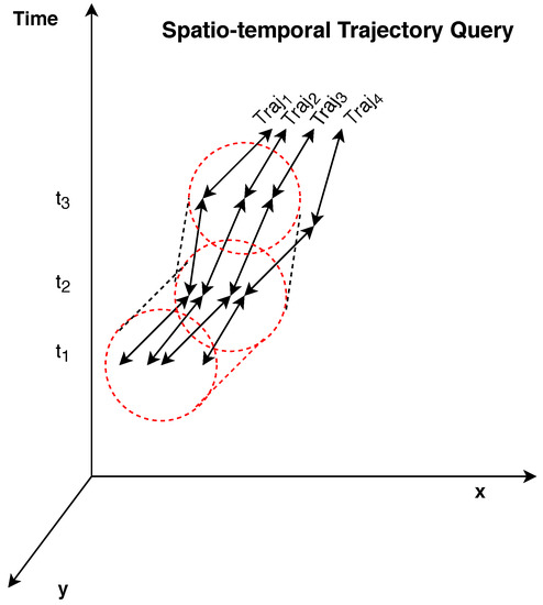
Figure 1. An Overview of Continuous Trajectory Point k Nearest Neighbor ($CTPkNN$) Query.

3.4. Problem Formulation

The problem of Robust Spatio-temporal Databases is addressed in an environment suitable for Big Spatial Data Management. The k-anonymization approach adopted in [30] for preventing mobile objects identity reveal, is related to k-NN algorithm as described in Section 3.2. Specifically, the k-anonymity set is formulated by the unique object identifier, denoted as $id$, of the k nearest neighbors, exploiting as a result the spatio-temporal data of a set of mobile objects.

Through the SMaRT system, a set of mobile users’ trajectory data is recorded per timestamp, that is, the mobile user trajectory $id$ and the values of longitude and latitude are recorded. From these location features, the four attributes $(x,y,\theta ,u)$ (as presented in Table 1) along with the values of Hough-X and Hough-Y of $(x,y)$ [9], $(U_x,a_x,U_y,a_y,b_x,w_x,b_y,w_y)$ (as presented in Table 2), are computed.

Table 1. An Overview of an Original Spatio-Temporal Database.

ID	Timestamp	Time to Next Point	x	y	Angle $\mathit{\theta }$	Velocity u
1	9 March 2013 10:00:01	0	21,082	56,436	1.23	0
1	9 March 2013 10:00:04	3	21,099	56,432	1.16	4.5
1	9 March 2013 10:00:11	7	21,221	56,484	1.51	14.6
1	9 March 2013 10:00:19	8	21,331	56,524	1.95	11.3
1	9 March 2013 10:00:21	2	21,402	56,495	0	29.5
2	9 March 2013 10:00:03	0	35,587	59,829	−2.76	0
2	9 March 2013 10:00:08	5	35,568	59,782	2.94	7.8
2	9 March 2013 10:00:16	8	35,580	59,723	−2.07	5.8
2	9 March 2013 10:00:25	9	35,530	59,668	−1.52	6.4
2	9 March 2013 10:00:34	9	35,476	59,671	−2.85	4.6

Table 2. An Overview of the Transformed Spatio-Temporal Database.

ID	Timestamp	${\mathit{U}}_{\mathit{x}}$	${\mathit{a}}_{\mathit{x}}$	${\mathit{U}}_{\mathit{y}}$	${\mathit{a}}_{\mathit{y}}$	${\mathit{b}}_{\mathit{x}}$	${\mathit{w}}_{\mathit{x}}$	${\mathit{b}}_{\mathit{y}}$	${\mathit{w}}_{\mathit{y}}$
1	9 March 2013 10:00:01	4.37	22,242,219.9	1.03	4,800,692.9	0.23	−5,093,637.76	0.97	−4,645,833.3
1	9 March 2013 10:00:04	13.4	22,242,156.2	5.83	4,800,651.2	0.075	−1,659,862.40	0.17	−82,3641.2
1	9 March 2013 10:00:11	10.58	22,242,287.4	3.79	4,800,713.7	0.0946	−2,103,289.59	0.26	−1,267,515.2
1	9 March 2013 10:00:19	27.3	22,242,427.4	11	4,800,762	0.04	−814,740.93	0.09	−436,432.91
1	9 March 2013 10:00:21	27.3	22,242,427.4	11	4,800,762	0.04	814,740.9	0.09	−436,432.91
2	9 March 2013 10:00:03	2.92	22,256,723.4	7.32	4,804,052.4	0.3425	−7,622,165.55	0.14	−-656,291.3
2	9 March 2013 10:00:08	1.15	22,256,709.8	5.75	4,803,996	0.87	−19,353,660.69	0.17	−835,477.56
2	9 March 2013 10:00:16	4.27	22,256,692.6	4.64	4,803,941.2	0.23	−5,216,411.92	0.22	−1,034,341.51
2	9 March 2013 10:00:25	4.6	22,256,639.5	0.23	4,803,925.9	0.22	−4,826,741.21	4.29	−20,588,283.27
2	9 March 2013 10:00:34	1.5	22,256,625.5	5.2	4,803,925.8	0.67	−14,837,750.3	0.19	−923,831.89

So, by employing the k-NN method for different pairs of features, this fact enables us to form the k-anonymity set of each mobile object per timestamp, as depicted in Table 3.

Table 3. k-Anonymity Sets for N Mobile Users in $L=5$ Timestamps.

ID	Time Moment	knns $\mathbf{id}$
1	1	$[i{d}_{111},i{d}_{112},\dots ,i{d}_{11k}]$
1	2	$[i{d}_{121},i{d}_{122},\dots ,i{d}_{12k}]$
1	3	$[i{d}_{131},i{d}_{132},\dots ,i{d}_{13k}]$
1	4	$[i{d}_{141},i{d}_{142},\dots ,i{d}_{14k}]$
1	5	$[i{d}_{151},i{d}_{152},\dots ,i{d}_{15k}]$
2	1	$[i{d}_{211},i{d}_{212},\dots ,i{d}_{21k}]$
2	2	$[i{d}_{221},i{d}_{222},\dots ,i{d}_{22k}]$
2	3	$[i{d}_{231},i{d}_{232},\dots ,i{d}_{23k}]$
2	4	$[i{d}_{241},i{d}_{242},\dots ,i{d}_{24k}]$
2	5	$[i{d}_{251},i{d}_{252},\dots ,i{d}_{25k}]$
…	…	…
…	…	…
N	1	$[i{d}_{N11},i{d}_{N12},\dots ,i{d}_{N1k}]$
N	2	$[i{d}_{N21},i{d}_{N22},\dots ,i{d}_{N2k}]$
N	3	$[i{d}_{N31},i{d}_{N32},\dots ,i{d}_{N3k}]$
N	4	$[i{d}_{N41},i{d}_{N42},\dots ,i{d}_{N4k}]$
N	5	$[i{d}_{N51},i{d}_{N52},\dots ,i{d}_{N5k}]$

For each mobile user i and per timestamp l, the k nearest neighbors $id$ it is computed and in the following is kept in a vector form $knn{s}_{il}=[i{d}_{il1}i{d}_{il2}\dots i{d}_{ilk}]$ for $l=1,2,\dots ,L$ as presented in Table 3. For each user, the number $k_s$ out of the k nearest neighbors, which remains the same from one timestamp to another, is computed in order to estimate the vulnerability ratio $\frac{1}{k_s}$. Hence, higher $k_s$ is associated with lower probability (i.e., lower vulnerability) a moving object’s identity being unveiled.

Definition 7.

k-anonymous database: A database is k-anonymous, i.e., its records are k-anonymous with respect to the selected features, if $k-1$ discrete records in the same specific timestamp τ, have at least the same nearest neighbors so that no record of k is distinguished from its $k-1$ neighboring records.

3.5. System Model

A spatio-temporal database is considered with N records, that is, N moving objects in the $xy$ plane. Each record $(x_i^j,y_i^j)$ represents the spatial coordinates of a mobile user j in timestamp $t_i^j$, or point i of its trajectory j [31]. From the location coordinates $(x,y)$, we can extract the corresponding velocity and angle direction features $(u,\theta )$ and the dual points $(U_x,a_x)$, $(U_y,a_y)$, $(b_x,w_x)$, $(b_y,w_y)$ by employing the dual methods described in [9]. Let us assume a trajectories database $T=\{T^1,\dots ,T^N\}$ of equal length L in which each trajectory is represented via a sequence of L triples.

For each point i in trajectory j, we define a two-dimensional feature vector $F_i^j$, which captures the selected features data. Hence, we can define and store the trajectory j as $T^j=\{F_1^j,F_2^j,F_3^j,\dots ,F_L^j\}$.

In the context of this work, the time performance of the k-anonymity set formulation either with the aid of an indexing method or for spatial k-NN queries on trajectory data employing Snapshot k-NN query on Trajectory Points, as depicted in Figure 2, is evaluated. Given a set of trajectories represented as a sequence of spatio-temporal points along with a query point, the $STPkNN$ algorithm finds its k nearest spatial points from a set of trajectory points in corresponding timestamps. The $STPkNN$ query is issued over a set of moving objects, executing the classical k-NN in a time period, and updates the k-anonymity set from timestamp to timestamp for all objects.

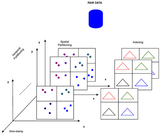
Figure 2. An Overview of Spatio-Temporal Data Partitioning and Indexing.

However, some objects may not move with the same velocity, leading to changes in the query result, i.e., in the k-anonymity set. As a result, in Privacy Preserving, it is important for the k-anonymity set to remain the same or vary slowly, as in this case, the vulnerability measure of moving objects will be affected. Note that, for a given STPkNN query q, the k-anonymity set, denoted as $\mathcal{A}$, should always satisfy the following conditions:

• The first condition $\left|\mathcal{A}\right|=k$ ensures that the anonymity set contains the $id$s of k objects.
• The second condition $\forall a\in (S-\mathcal{A}),dist(q,a)\ge maxdist(q,a)|a\in \mathcal{A}$ ensures that these k objects’ $id$ are the k nearest ones to q.

Assuming a mobile object when considering a k-NN query relevant to the selected features in a specific timestamp, then, the spatial k-anonymity ensures that an attacker, as the query issuer, cannot identify a mobile object with probability larger than $\frac{1}{k}$, where k is a user-defined anonymity parameter. Moreover, a spatio-temporal database is expected to handle a high number of moving objects location data, as well as, a large number of consecutive k-NN queries. Hence, an efficient consecutive $STPkNN$ processing algorithm is very important to be addressed. To this end, the $STPkNN$ query is investigated in the GeoSpark framework and experimental evaluations are conducted using a realistic dataset to demonstrate the time performance of the k-anonymity set computation under the $STPkNN$ query. Ultimately, the vulnerability behavior for different pairs of features is investigated.

3.6. GeoSpark System Overview

In this subsection, the necessary structures of GeoSpark-based approach is thoroughly presented. All parts were implemented using Apache Scala due to its compatibility with Apache Spark framework. The core components are the following implemented on GeoSpark Resilient Distributed Dataset (RDD) and the interaction with GeoSpark is utilized through Apache Zeppelin interface.

3.6.1. GeoSpark Architecture

GeoSpark [32] is an extension of the Apache Spark core and provides additional tools to manage geospatial data, e.g., geospatial datatypes, indexes and operations. The architecture of GeoSpark, as introduced in Figure 3, consists of the following three layers:

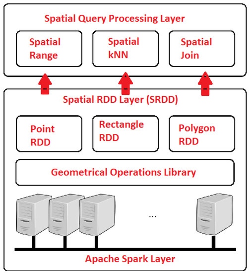
Figure 3. An Overview of GeoSpark Layers.

• The Apache Spark Layer consists of all the components present in Spark and performs data loading and querying.
• The Geospatial RDD Layer extends Spark and supports three types of RDD, i.e., Point, Rectangle and Polygon RDD. In addition, it contains a geometrical operations library for every RDD.
• The Geospatial Query Processing Layer is used to perform different types of geospatial queries.

GeoSpark provides Spatial RDD that allows efficient loading, transformation, partitioning, in-memory storing as well as indexing of complex spatial data for different input data sources such as CSV, WKT, GeoJSON, Shapefile, etc., which, through the GeoSpark Spatial SQL interface, are compatible with Spark. It also provides eight types of spatial objects, namely Point, Multi-Point, Polygon, Multi-Polygon, Line String, Multi-Line String, GeometryCollection, and Circle. Hence, spatial objects in a Spatial RDD can consist of different geometry types. Furthermore, it supports three types of spatial objects, which are Point, Rectangle and Polygon, for which the corresponding spatial RDDs can be defined. These structures can be used as input to several spatial queries, such as spatial k-NN, spatial range and spatial join.

In following, taking advantage of the GeoSpark architecture, the main parts of our approach will be presented.

3.6.2. Spatial RDD Structures Preparation

Initially, the trajectory data of all mobile users is stored in a csv file. Specifically, this data consists of trajectory (spatio-temporal) points for a number of mobile objects, i.e., bike riders. For each bike trajectory (spatio-temporal) point, we have in our disposal the bike rider $id$, the spatial coordinates $(x,y)$, the polar coordinates (direction, velocity) $(u,\theta )$, the Hough-$X/Y$ attributes as well as the timestamp, with the aim of computing the k nearest neighbors and selecting two features among them, at each time. Practically, all bike riders follow non-linear trajectories. However, in our case, the users’ trajectory is approximated by linear sub-trajectories, as, in our previous work [9], thus, the values of the attributes are not randomized such that groups of bikes have similar behavior. The user cannot control attribute values, but, they may ask to simulate a specific timestamp. In GeoSpark, firstly the corresponding $SRDD$ is recovered and in following the temporal partitioning is implemented. Information about road network that describe the situation of the region are not taken into consideration.

In Apache Zeppelin, the input data are loaded from the csv file as a Dataframe and then SQL queries can be executed on the created Dataframe in order to recover spatial data of moving objects in specific timestamps. Then, these data are stored and transformed to PointRDD. In this way, several PointRDDs are created which, from now, will be called as BikesRDD, as they concern bike riders trajectories (spatio-temporal points). GeoSpark’s operator permits us to transform a set of raw data into a PointRDD, and selecting the columns that correspond to the desired features at a specific timestamp, as depicted in Table 4.

Table 4. The Different Types of Point Resilient Distributed Dataset (RDDs) According to Selected Features.

PointRDDs
Features	Type of PointRDD
$(x,y)$	Spatial Points RDD
$(u,\theta )$	Polar Points
$(a_x,U_x)$	Hough-X of x PointRDD
$(a_y,U_y)$	Hough-X of y PointRDD
$(b_x,w_x)$	Hough-Y of x PointRDD
$(b_y,w_y)$	Hough-Y of y PointRDD

3.6.3. Spatio-Temporal Partitioning

The proposed approach considers a naive temporal partitioning from which a collection of timestamps is considered. These timestamps are related to the sampling period where the system recorded the spatio-temporal data with its usage. As a result, the size of the loaded data in BikesRDD may be different for different timestamps since some mobile objects may not have a spatio-temporal footprint for all recorded timestamps. Here, in our simulations, the sampling period is supposed to be similar for all bike riders trajectory data. From the trajectory (i.e., spatio-temporal) points of a number of bike riders objects at different timestamps, a collection of BikesRDD is constructed.

Following the previous aspects, GeoSpark can easily utilize spatial partitioning over the temporal partition of the data of these bikes. In each temporal partition, a bike rider may have not necessarily moved because random delays may be employed. Hence, in a specific time partition, the spatial data of all bikes may not necessarily participate.

BikesRDD constitutes a specialized GeoSpark PointRDD, which consists of individual bike riders’ records. The spatial partitioning on the BikesRDD concerns bike riders selected features, such as the location data. In several temporal partitions, the BikesRDD are simulated one by one.

More to the point, GeoSpark offers low overhead spatial partitioning approaches that take into consideration the spatial distribution of the data as well as repartitions a loaded Spatial RDD in an automatic way. In each Spatial RDD, several spatially proximal objects are grouped into the same partition and, as a result, the partitioning layer in GeoSpark partitions the workload in a spatial way and periodically repartitions this workload in order to keep balanced partitions. Also, it supports a variety of grid-type partitioning methods, such as equal-grids, R-tree, Quad-tree and $KDB$-tree, to name a few [33].

3.6.4. k-Anonymity Set in GeoSpark

Algorithm 1 presents the steps of a spatial k-NN in GeoSpark. It takes as input a non-indexed or indexed $SRDD$, a query center point as well as a parameter k, which indicates the number of nearest neighbors. The algorithm is separated in two phases, namely selection and sorting phase [33], and will be utilized in the simulations.

Algorithm 1 Spatial k-NN Query

1: input The number of k nearest neighbors 2: input A query center object A 3: input A Spatial RDD B 4: output A list of k spatial objects 5: Step 1: Selection phase 6: for all partition ∈ SRDD B do 7:  if an index exists then 8:   Return k-neighbors of A by querying the index of this partition 9:  else 10:   for all object ∈ this partition do 11:    Check all the distance between the object A and Spatial RDD B 12:   end for 13:  end if 14: end for 15: Maintain a priority queue that stores the top k nearest neighbors 16: Step 2: Sorting phase 17: Sort the spatial objects in the intermediate Spatial RDD based on their distances to A 18: Return top k objects in C

Our aim is to exploit the above mentioned structures and Algorithm 1 so as to formulate the k-anonymity set for a number of moving objects based on their trajectory (spatio-temporal) data. From the trajectory points of a number of mobile objects at different timestamps, a collection of spatial BikesRDD is constructed. The goal of this paper is to provide an efficient and scalable framework for robust continuous k-NN querying of spatial objects in GeoSpark. A Scala RDD API for creating the desired PointRDD from a csv file is introduced in following Algorithm 2.

Algorithm 2 Spatial PointRDD Creation

1: Define csv file location in pointRDDInputLocation 2: Define the attributes start Column equal to 0 in pointRDDOffset 3: Define pointRDDSplitter as FileDataSplitter.csv 4: Define rest attributes in carryOtherAttributes = true 5: Create PointRDD: PointRDD = new PointRDD(sc, pointRDDInputLocation, pointRDDOffset, pointRDDSplitter, carryOtherAttributes)

An iterative application of a typical spatial k-NN query, which was presented in Algorithm 1, is introduced with use of Scala RDD API of Geospark in following Algorithm 3.

Algorithm 3 Iterative Spatial k-NN Query

1: inputk, usingIndex, number of timestamps L 2: for timestamp $t=1$ to L do 3:  Create the Dataframe $df$ with the selected features in t 4:  Save $df$ as csv file f 5:  Create from csv a PointRDD 6:  if usingIndex = true then 7:   Build R-Tree index on PointRDD 8:  end if 9:  for all lines ∈ csv file f do 10:   Read the selected features $(f_1,f_2)$ 11:   Create querypoint 12:   val fact = new GeometryFactory() 13:   val querypoint = fact.createPoint(new Coordinate($f_1$,$f_2$)) 14:   Run Spatial k-NN Query to return k geometry points 15:   val queryResultList = KNNQuery.SpatialKnnQuery(PointRDD, querypoint, k, usingIndex) 16:  end for 17: end for

It is worth mentioning the fact that the output format of the spatial k-NN query (indexed or not) is a list of geometries as in Table 5, where the $id$ of the point geometry is related to the mobile object $id$. In addition, the list holds the top-k geometry objects. In the following, the above methodology and algorithms will be considered for the performance evaluation of the proposed k-anonymity method based on spatial k-NN.

Table 5. Trajectory Representation in a PointRDD.

Trajectory Points
Point ($-88.331492,32.324142$)
Point ($-88.175933,32.360763$)
Point ($-88.388954,32.357073$)
Point ($-88.221102,32.35078$)

4. Results

4.1. Environment and Dataset

A local machine was used for the experimental evaluation. The experiments were executed using 1 VM, which consisted of 4 CPU Cores, $3.8$ Gb RAM and 488 Gb Storage capacity each with Ubuntu $\mathrm{18.04.4}$ LTS, Apache Spark $\mathrm{2.1.0}$, GeoSpark $\mathrm{1.2.0}$ and Apache-Zeppelin $\mathrm{0.8.2}$. We conducted the experiments on one master node and assign $384.1$ MB memory to the Spark driver program that is executed on the master local machine. The experimental data extracted from the SMaRT Database GIS Tool (http://www.bikerides.gr/thesis2/). The experiments were based on trajectory datasets of bike riders in the area of Corfu, Greece, so the case study area is located in the non-urban area of Corfu.

4.2. Time Performance of k-Anonymity Set

A comprehensive experimental evaluation that studies the performance of GeoSpark under the studying problem, lies in the corresponding subsection. Specifically, the GeoSpark spatial k-NN query performance, which impacts the computation of the k-anonymity set of 80, 500 as well as 2000 mobile objects in 10 consecutive timestamps, as shown in Table 6, is measured. The spatial k-NN queries are tested by varying k values equal to 8 and 16 on Bike Riders Trajectory (spatio-temporal points) dataset. The performance measure of the system for the k-anonymity set computation is the total run time that the system needs to execute the jobs. We compare the following spatial data processing approaches:

Table 6. Simulation Parameters.

Parameters
Parameter	Range
Mobile Objects	80, 500, 2000
Timestamps	10
Time Step	uniform

• Without Partitioning–Without Indexing: GeoSpark approach without spatial index in non-partitioned PointRDD.
• Without Partitioning–With Indexing: GeoSpark approach with spatial index in non-partitioned PointRDD.
• With Partitioning–Without Indexing: GeoSpark approach with spatial index on each partition of PointRDD after data partitioned according grids using (i) KDB-Tree and (ii) R-Tree.

The above cases will be taken into consideration in order to evaluate the GeoSpark performance for the computation of the k-anonymity set for a number of mobile users. To form the desired k-anonymity set, we apply spatial k-NN queries using the embedded function known as ”KNNQuery.SpatialKnnQuery”. The spatial index R-tree is only supported for the spatial k-NN Queries.

We consider the following results assuming that the trajectories are represented as a collection of spatio-temporal points in two-dimensional space. The experiments were conducted in Apache Zeppelin, which is an open web-based notebook that enables interactive data analytics. In Figure 4, an SQL query is employed, which returns the trajectory data (spatio-temporal points) of 40 mobile objects. Specifically, a notebook, created in Zeppelin through which the methods described in previous section were executed under GeoSpark framework, is utilized.

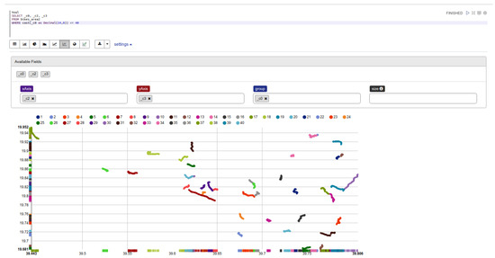
Figure 4. An Overview of 40 Trajectories through Zeppelin.

In this case, it should be noted that the experimentation depicts that, when mobile objects do not move at the same timestamps, then it is difficult for the k-anonymity set to be formed, as the desired set of mobile objects has very low cardinality. Also, we observed that from timestamp to timestamp, different objects participated in the formed dataset, meaning that the k nearest neighbors are time-varying. Such a scenario proves that the randomness in objects’ movements does not benefit or promote the formulation of a slow time-varying anonymity set, as we have proved in our previous work [30].

4.2.1. Impact of Data Size

In this subsection, the impact of data size in terms of the number of mobile objects N in Figure 5 and storage size in MB in Figure 6 with or without the aid of an R-Tree indexing on the computation time of the k-anonymity set are investigated. According to results in Table 7, Table 8 and Table 9, we observe that the use of indexing does not impact the total execution time of involved spatial k-NN queries. This happens due to the fact that GeoSpark caches the spatial RDD along with the corresponding indexes in each timestamp. Hence, for the upcoming mobile objects, it directly reads spatial PointRDD and index from the cache, in this way leading to time saving. It should be also noted that in each timestamp, all objects use the same (partitioned or not) PointRDD, which changes in the upcoming timestamps for all the objects.

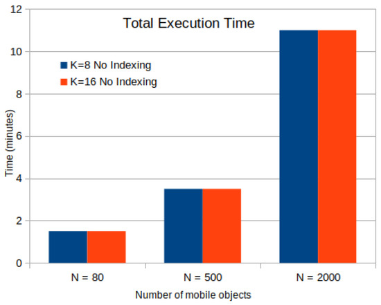
Figure 5. Time Cost for k-Anonymity Set Computation with or without Indexing for $N=80,500,2000$ Mobile Objects.

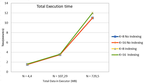
Figure 6. Time Cost for k-Anonymity Set Computation with or without Indexing for 3 Cases of Total Input Data in Executor.

Table 7. Time for 80 Mobile Objects without Indexing and with R-Tree Indexing.

Time Results in Minutes
k-NNs	No Indexing	Indexing	Number of Completed Jobs	Number of Queries
8	1.5	1.6	730	6400
16	1.5	1.6	730	6400

Table 8. Time for 500 Mobile Objects without Indexing and with R-Tree Indexing.

Time Results in Minutes
k-NNs	No Indexing	Indexing	Number of Completed Jobs	Number of Queries
8	3.5	3.6	4510	$25\times {10}^5$
16	3.5	3.6	4510	$25\times {10}^5$

Table 9. Time for 2000 Mobile Objects without Indexing and with R-Tree Indexing.

Time Results (Minutes)
k-NNs	No Indexing	Indexing	Number of Completed Jobs	Number of Queries
8	11	12	18,010	$4\times {10}^7$
16	11	12	18,010	$4\times {10}^7$

In terms of total execution time, as shown in Figure 5 including the time for index building on PointRDD, GeoSpark without index shows approximately similar search time performance as in the indexed version. Also, the execution time of a k-NN query in GeoSpark remains constant for different values of k in each case. That is mainly considered when the value of k is very small with respect to the input data and thus, most of the time is spent on input data processing. The time cost of loading data from csv to dataframe is 42 s whereas it is included in the total execution time.

Figure 6 illustrates the total execution time relative to the total input data size in executor in MB, which seems to increase in a non-linear way.

Ultimately, in Figure 7 let us focus only on higher number of mobile objects in order to understand the impact of data scalability in the time performance of the proposed approach for the k-anonymity set computation assuming 2-dimensional ($2D$) points RDD for 10 consecutive timestamps. Indeed, it seems to approach exponential increase which for actual Big Data will be more apparent.

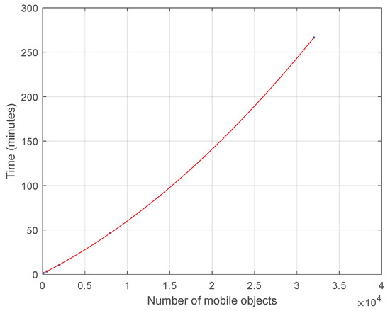
Figure 7. Time Cost for Mobile Objects $N=\{500,2000,8000,32.000\}$ without Indexing for $k=8$.

4.2.2. Impact of Spatial Partitioning

In this subsection, we experiment on the impact of the embedded spatial partitioning methods on the computation time of k-anonymity set, despite the fact that in GeoSpark the spatial partitioning method is usually used to optimize spatial join.

Initially, in Figure 8, the total number of records in PointRDDs for four partitioning methods in a specific timestamp is demonstrated. Obviously, the partition size of $KBD$-Tree partitioning is more balanced than that of Quad-Tree. Also, we observe that regarding R-Tree partitioning, an overflow in data partition (e.g., partition 2) occurs, which is much larger than other partitions because R-Tree does not consider the whole space [33].

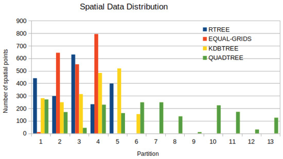
Figure 8. Spatial PointRDD Data Distribution for 4 Spatial Partition Techniques for 2000 Mobile Objects.

Note that, in the third dataset, with size $N=2000$, the data distribution varies from one timestamp to another and thus, it is not recorded in Table 10.

Table 10. Impact of Spatial Partitioning in Time Performance.

Time Results (Minutes) for Different Spatial Partitioning Methods
Mobile Objects	R-Tree	$KDB$-Tree	Completed Jobs
N = 80	1.4	1.5	766
N = 500	3.6	3.7	4546
N = 2000	12	12	18,046
Data Distribution for 2 Different Spatial Partitioning Methods
Mobile Objects	R-Tree	KDB-Tree
N = 80	40 40 0	30 25 25
N = 500	250 250 0	236 132 132

In Table 10, we focus only on the impact of R-Tree and $KDB$-Tree spatial partitioning on k-anonymity set time computation without PointRDD indexing, as GeoSpark does not support building local indexing on spatially partitioned data for spatial k-NN queries.

We choose to evaluate, for a specific k with value equal to 16, the impact of spatial data partitioning on the time needed to formulate the k-anonymity set for 10 consecutive timestamps, as aforementioned. As the results show, the time cost of the k-anonymity method did not benefit from data partitioning. In addition, the time for the k-anonymity set computation is a little bit lower when using R-Tree for datasets having smaller size. However, in case of a larger dataset, the difference between the two types of partitioning is normalized. This means that most of the processing time, in the same machine, is focused on k-NN query computation.

4.3. Vulnerability Evaluation

In this subsection, some additional experiments based on a real dataset with parameters presented in Table 11 and Figure 9, Figure 10 and Figure 11, are conducted. The k-anonymity set computation is utilized with the aid of R-Tree indexing. As GeoSpark works with spatial data in two-dimensional space, our focus is on three different cases for the k-anonymity set computation in order to evaluate the vulnerability under the formulated anonymity set in each space, which are:

Table 11. Parameters when using $N=500$ Trajectories, $L=100$ Timestamps.

Anonymity Set Size k	Anonymity Set Attributes
5, 10	$(x,0)$
5, 10	$(0,y)$
5, 10	$(x,y)$
5, 10	$(U_x,a_x)$
5, 10	$(U_y,a_y)$

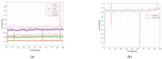
Figure 9. (a) Euclidean Space and (b) Polar Space for $N=500$ Trajectories, $L=100$ Timestamps.

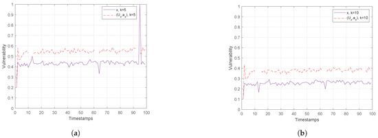
Figure 10. Hough-X Space of x for (a) $k=5$ and (b) $k=10$ for $N=500$ Trajectories, $L=100$ Timestamps.

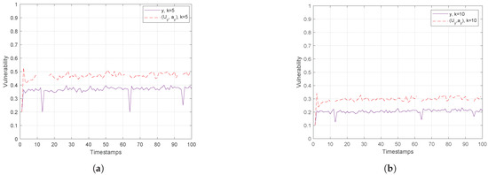
Figure 11. Hough-X Space of y for (a) $k=5$ and (b) $k=10$ for $N=500$ Trajectories, $L=100$ Timestamps.

• Euclidean coordinates $(x,y)$
• Polar coordinates $(u,\theta )$
• Hough-X coordinates of $(x,y)$ denoted as $(U_x,a_x)$ and $(U_y,a_y)$

The experimentation has been carried out on a dataset of size $N=500$ Trajectories (or moving objects).

Actually, Figure 9 on the left depicts that assuming only the x feature (or y one) for the anonymity set formulation, the vulnerability in both cases is about 2 times higher than in the case when both attributes $(x,y)$ are considered. Similarly, in Figure 9 on the right, the vulnerability is measured in polar space, where the performance is worse than in Euclidean one. This is attributed to the fact that polar coordinates are linearly dependent on spatial data $(x,y)$, revealing the curse of dimensionality. Also, this figure reveals that the anonymity set varies from timestamp to timestamp, meaning that for given objects angle direction and velocity, more than one out of k nearest neighbors change.

Finally, Figure 10 and Figure 11 show the vulnerability performance in Hough-X space, which is compared with the corresponding one in Euclidean space. Obviously, the results are better in Euclidean space as Hough-X space is linearly dependent on the former. Finally, focusing on the case where $k=10$ in Figure 12, the vulnerability varies slowly around $0.4$ and $0.3$ (red and orange dashed lines respectively) in Hough-X space, while in Euclidean space, it achieves values very close to $0.1$ (purple solid lines).

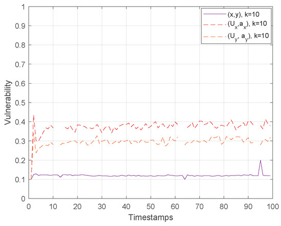
Figure 12. Vulnerability Performance Comparison in Euclidean and Hough-X Space.

5. Discussion

In this section, two main issues will be discussed. At first, the time performance of the researched issue and in following the robustness of the suggested anonymity method. Actually, the analysis in Section 4 gives some useful insights and presents some key aspects of the results obtained from the evaluation of the proposed k-anonymity method in GeoSpark.

5.1. Performance Issues

Here, we should claim that the adopted partitioning method is simple. Hence, to improve the performance of the suggested privacy preserving $CkNN$s, we could employ the approach proposed in [34] and extend Algorithm 1 by applying the smart partitioning technique. Especially, we could consider to compute $AkNN$ queries based on $kdANN$ or $kdANN+$ (where d stands for the dimensionality), instead of simple k-NN queries and study the effect of d on the performance of such queries and thus, in k-anonymity set computation performance, which is the main issue in the context of this research work. At this point, it should be noted that that approach exploits a space decomposition technique suitable for Big Data and processes the classification in a parallel and distributed manner considering multidimensional objects, as well. Through an extensive experimental evaluation it has been proved that the solution is efficient, robust and scalable in processing the k nearest neighbor queries.

Although the trajectory (spatio-temporal) data utilized in this article are 2-dimensional (2D), the methodology and techniques are general and applicable to higher dimensions. Hence, observing Figure 5 and Figure 6 in Section 4, the efficiency of the proposed approach, which now is investigated utilizing 2D trajectory (spatio-temporal) points datasets, is expected to scale up exponentially with respect to both data size, as shown in Figure 7, and dimensions, when $d>2$, in the same trend as in [34]. This results from the curse of dimensionality. As the number of dimensions increases, the number of distance computations as well as the number of searches. For further experimentation with the dimensionality parameter $d>2$ in the context of GeoSpark, functions for data preprocessing to prepare Points RDD structure need to be redefined. Let us recall that GeoSpark RDD operations and k-NN queries processing work with 2D points.

Finally, as the previous finding shows in [34], it is expected that the increment of computing nodes (VMs) will improve scalability and time performance in support of both snapshot and continuous spatial queries over moving objects, having a great effect when the data follows a uniform distribution due to better load balancing. Indeed, the increment of number of computing nodes decreases the amount of distance calculations and update steps on k-NN lists that each computing node undertakes. A similar behavior we expect to see in our case if the processing is distributed in multiple nodes in the GeoSpark environment.

5.2. Vulnerability

Vulnerability is considered a major issue which arises in spatio-temporal data management as well, and simply measures how vulnerable various mobile objects are to revealing their identity to potential adversaries, when moving from one position to another. Moreover, reducing vulnerability and enhancing resilience in the face of adversity are considered to be essential steps. To date, less attention has been given to vulnerability resulting from k-NN querying on non-linear trajectory data.

This study investigates the vulnerability of mobile objects with respect to k-NN queries based on their geolocation data attributes. The proposed anonymity technique, as well as previous findings, are confirmed in the GeoSpark environment and, as a result, vulnerability is estimated for different risk conditions (i.e., for different number of nearest neighbors, namely k and pair of features, as presented in Table 4 and Table 11).

Furthermore, it is observed that for low values of k, the vulnerability remained at the medium level, and the more the nearest neighbors are utilized to form the anonymity set, the lower the vulnerability becomes. In other words, the results of the present study indicate a low level of vulnerability for high number of nearest neighbors and uncorrelated features data.

At this point, it should be noted that the results in Section 4 highlight the superiority, that is lower vulnerability, of Euclidean space in terms of privacy preserving, which is the main issue in k-anonymity and, thus, in applying robust k-NN queries. However, let us recall that, as it has been already investigated in [9], dual representative features, e.g., Hough-X of x and/or y, are considered an appropriate choice to form the k-anonymity set from both privacy preserving and storage efficiency perspective. So, priority should be given to the use of low dimension independent features data; in that case, the utilization of dual space against the Euclidean one.

6. Conclusions and Future Work

In conclusion, this work aimed at testing the hardware and software performance in terms of the number of operations performed and the time needed to obtain satisfactory anonymity. The real world example concerning moving bicycle riders proved satisfactory results using different additional ancillary methods of space partitioning and indexing. Also, a GeoSpark-based approach for evaluating the vulnerability of spatial k-anonymity in large-scale spatio-temporal data is provided. Experiments show that GeoSpark constitutes an appropriate Spark-based system for the evaluation of robust k-NN queries. The GeoSpark spatial RDDs are exploited to store trajectory data of the mobile objects as PointRDD in order to acquire the anonymity sets of all query mobile objects issuing iterative spatial k-NN queries for all mobile objects in consecutive timestamps. It should be noted that the experiments were conducted in one Virtual Machine (VM) in local mode, with specific capabilities as described in the experimental evaluation.

As a future work, our aim is to apply the proposed anonymity method in a fully distributed environment with many VMs so as to verify the expected results from previous findings about the execution time; in this case, the input data will be partitioned and in following distributed to different VMs. In this way, several parallel tasks will be executed and thus, the execution time for the anonymity set computation is expected to be much lower than in the current single VM case when considering large-scale databases. The locality of the data and load balancing are important when applying efficient k-NN queries. GeoSpark also provides a grid-type partitioning based on $KDB$-tree that can ensure workload balancing.

In conclusion, it should be pointed out that the current experimentation gave us an insight about the design issues and possible constraints of the proposed approach so as to optimize its performance in terms of execution time cost and memory utilization for real-time scenarios, where the mobile objects identity security, when issuing a k-NN query, is of high importance.

References

- Jiang, F.; Leung, C.K. A Data Analytic Algorithm for Managing, Querying, and Processing Uncertain Big Data in Cloud Environments. Algorithms 2015, 8, 1175–1194. [Google Scholar] [CrossRef]
- Emani, C.K.; Cullot, N.; Nicolle, C. Understandable Big Data: A Survey. Comput. Sci. Rev. 2015, 17, 70–81. [Google Scholar] [CrossRef]
- Yang, C.; Yu, M.; Hu, F.; Jiang, Y.; Li, Y. Utilizing Cloud Computing to Address Big Geospatial Data Challenges. Comput. Environ. Urban Syst. 2017, 61, 120–128. [Google Scholar] [CrossRef]
- Shekhar, S.; Jiang, Z.; Ali, R.Y.; Eftelioglu, E.; Tang, X.; Gunturi, V.M.V.; Zhou, X. Spatiotemporal Data Mining: A Computational Perspective. ISPRS Int. J. Geo-Inf. 2015, 4, 2306–2338. [Google Scholar] [CrossRef]
- Güting, R.H.; Behr, T.; Xu, J. Efficient k-Nearest Neighbor Search on Moving Object Trajectories. VLDB J. 2010, 19, 687–714. [Google Scholar] [CrossRef]
- Huang, Y.; Chen, Z.; Lee, C. Continuous K-Nearest Neighbor Query over Moving Objects in Road Networks. In Proceedings of the Joint International Conferences on Advances in Data and Web Management (APWeb/WAIM), Suzhou, China, 2–4 April 2009; pp. 27–38. [Google Scholar]
- Fan, P.; Li, G.; Yuan, L. Continuous K-Nearest Neighbor Processing based on Speed and Direction of Moving Objects in a Road Network. Telecommun. Syst. 2014, 55, 403–419. [Google Scholar] [CrossRef][Green Version]
- Zheng, B.; Zheng, K.; Xiao, X.; Su, H.; Yin, H.; Zhou, X.; Li, G. Keyword-Aware Continuous kNN Query on Road Networks. In Proceedings of the 32nd IEEE International Conference on Data Engineering (ICDE), Helsinki, Finland, 16–20 May 2016; pp. 871–882. [Google Scholar]
- Dritsas, E.; Kanavos, A.; Trigka, M.; Sioutas, S.; Tsakalidis, A.K. Storage Efficient Trajectory Clustering and k-NN for Robust Privacy Preserving Spatio-Temporal Databases. Algorithms 2019, 12, 266. [Google Scholar] [CrossRef]
- Huang, Y.; Lee, C. Efficient Evaluation of Continuous Spatio-temporal Queries on Moving Objects with Uncertain Velocity. GeoInformatica 2010, 14, 163–200. [Google Scholar] [CrossRef]
- Fan, P.; Li, G.; Yuan, L.; Li, Y. Vague Continuous K-Nearest Neighbor Queries over Moving Objects with Uncertain Velocity in Road Networks. Inf. Syst. 2012, 37, 13–32. [Google Scholar] [CrossRef]
- Heendaliya, L.; Lin, D.; Hurson, A.R. Continuous Predictive Line Queries for On-the-Go Traffic Estimation. Trans. Large-Scale Data Knowl.-Cent. Syst. 2015, 18, 80–114. [Google Scholar]
- Wu, W.; Parampalli, U.; Liu, J.; Xian, M. Privacy Preserving K-Nearest Neighbor Classification over Encrypted Database in Outsourced Cloud Environments. World Wide Web 2019, 22, 101–123. [Google Scholar] [CrossRef]
- Yang, S.; Tang, S.; Zhang, X. Privacy-Preserving K-Nearest Neighbor Query with Authentication on Road Networks. J. Parallel Distrib. Comput. 2019, 134, 25–36. [Google Scholar] [CrossRef]
- Hagedorn, S.; Götze, P.; Sattler, K. The STARK Framework for Spatio-Temporal Data Analytics on Spark. In Proceedings of the 17th Conference on Database Systems for Business, Technology, and Web (BTW), Stuttgart, Germany, 6–10 March 2017; Volume P-265, pp. 123–142. [Google Scholar]
- Hagedorn, S.; Räth, T. Efficient Spatio-Temporal Event Processing with STARK. In Proceedings of the 20th International Conference on Extending Database Technology (EDBT), Venice, Italy, 21–24 March 2017; pp. 570–573. [Google Scholar]
- Zhang, Z.; Jin, C.; Mao, J.; Yang, X.; Zhou, A. TrajSpark: A Scalable and Efficient In-Memory Management System for Big Trajectory Data. In Proceedings of the 1st (APWeb-WAIM) International Joint Conference on Web and Big Data, Beijing, China, 7–9 July 2017; pp. 11–26. [Google Scholar]
- Alarabi, L. Summit: A Scalable System for Massive Trajectory Data Management. In Proceedings of the 26th ACM SIGSPATIAL International Conference on Advances in Geographic Information Systems (SIGSPATIAL), Seattle, WA, USA, 6–9 November 2018; pp. 612–613. [Google Scholar]
- Giannousis, K.; Bereta, K.; Karalis, N.; Koubarakis, M. Distributed Execution of Spatial SQL Queries. In Proceedings of the IEEE International Conference on Big Data, Seattle, WA, USA, 10–13 December 2018; pp. 528–533. [Google Scholar]
- Patrou, M.; Alam, M.M.; Memarzia, P.; Ray, S.; Bhavsar, V.C.; Kent, K.B.; Dueck, G.W. DISTIL: A Distributed In-Memory Data Processing System for Location-Based Services. In Proceedings of the 26th ACM SIGSPATIAL International Conference on Advances in Geographic Information Systems, Seattle, WA, USA, 4–6 November 2018; pp. 496–499. [Google Scholar]
- Yang, C.; Yu, X.; Liu, Y. Continuous KNN Join Processing for Real-Time Recommendation. In Proceedings of the IEEE International Conference on Data Mining (ICDM), Shenzhen, China, 14–17 December 2014; pp. 640–649. [Google Scholar]
- Huang, Y. Processing KNN Queries in Grid-Based Sensor Networks. Algorithms 2014, 7, 582–596. [Google Scholar] [CrossRef]
- Dong, T.; Lulu, Y.; Shang, Y.; Ye, Y.; Zhang, L. Direction-Aware Continuous Moving K-Nearest-Neighbor Query in Road Networks. ISPRS Int. J. Geo-Inf. 2019, 8, 379. [Google Scholar] [CrossRef]
- Wang, Y.; Xia, Y.; Hou, J.; Gao, S.; Nie, X.; Wang, Q. A Fast Privacy-Preserving Framework for Continuous Location-based Queries in Road Networks. J. Netw. Comput. Appl. 2015, 53, 57–73. [Google Scholar] [CrossRef]
- Song, D.; Park, K. A Privacy-Preserving Location-Based System for Continuous Spatial Queries. Mob. Inf. Syst. 2016, 2016, 6182769:1–6182769:9. [Google Scholar] [CrossRef]
- Zhang, S.; Mao, X.; Choo, K.R.; Peng, T.; Wang, G. A Trajectory Privacy-Preserving Scheme Based on Dual-K Mechanism for Continuous Location-Based Services. Inf. Sci. 2020, 527, 406–419. [Google Scholar] [CrossRef]
- Eldawy, A.; Alarabi, L.; Mokbel, M.F. Spatial Partitioning Techniques in Spatial Hadoop. Proc. VLDB Endow. 2015, 8, 1602–1605. [Google Scholar] [CrossRef]
- Yu, Z.; Liu, Y.; Yu, X.; Pu, K.Q. Scalable Distributed Processing of K Nearest Neighbor Queries over Moving Objects. IEEE Trans. Knowl. Data Eng. 2015, 27, 1383–1396. [Google Scholar] [CrossRef]
- García-García, F.; Corral, A.; Iribarne, L.; Vassilakopoulos, M. Improving Distance-Join Query processing with Voronoi-Diagram based partitioning in SpatialHadoop. Future Gener. Comput. Syst. 2019, 111, 723–740. [Google Scholar] [CrossRef]
- Dritsas, E.; Trigka, M.; Gerolymatos, P.; Sioutas, S. Trajectory Clustering and k-NN for Robust Privacy Preserving Spatiotemporal Databases. Algorithms 2018, 11, 207. [Google Scholar] [CrossRef]
- Yuan, G.; Sun, P.; Zhao, J.; Li, D.; Wang, C. A Review of Moving Object Trajectory Clustering Algorithms. Artif. Intell. Rev. 2017, 47, 123–144. [Google Scholar]
- Huang, Z.; Chen, Y.; Wan, L.; Peng, X. GeoSpark SQL: An Effective Framework Enabling Spatial Queries on Spark. ISPRS Int. J. Geo-Inf. 2017, 6, 285. [Google Scholar] [CrossRef]
- Yu, J.; Zhang, Z.; Sarwat, M. Spatial Data Management in Apache Spark: The GeoSpark Perspective and Beyond. GeoInformatica 2019, 23, 37–78. [Google Scholar] [CrossRef]
- Nodarakis, N.; Pitoura, E.; Sioutas, S.; Tsakalidis, A.K.; Tsoumakos, D.; Tzimas, G. kdANN+: A Rapid AkNN Classifier for Big Data. Trans. Large-Scale Data Knowl.-Cent. Syst. 2016, 24, 139–168. [Google Scholar]
© 2020 by the authors. Licensee MDPI, Basel, Switzerland. This article is an open access article distributed under the terms and conditions of the Creative Commons Attribution (CC BY) license (http://creativecommons.org/licenses/by/4.0/).