Abstract
Traditional time-series clustering methods usually perform poorly on high-dimensional data. However, image clustering using deep learning methods can complete image annotation and searches in large image databases well. Therefore, this study aimed to propose a deep clustering model named GW_DC to convert one-dimensional time-series into two-dimensional images and improve cluster performance for algorithm users. The proposed GW_DC consisted of three processing stages: the image conversion stage, image enhancement stage, and image clustering stage. In the image conversion stage, the time series were converted into four kinds of two-dimensional images by different algorithms, including grayscale images, recurrence plot images, Markov transition field images, and Gramian Angular Difference Field images; this last one was considered to be the best by comparison. In the image enhancement stage, the signal components of two-dimensional images were extracted and processed by wavelet transform to denoise and enhance texture features. Meanwhile, a deep clustering network, combining convolutional neural networks with K-Means, was designed for well-learning characteristics and clustering according to the aforementioned enhanced images. Finally, six UCR datasets were adopted to assess the performance of models. The results showed that the proposed GW_DC model provided better results.
1. Introduction
Time-series clustering [1,2], just like time-series classification [3] and time-series prediction [4,5], is one of the data mining methods of time-series. Time-series clustering is used to extract useful information from the data curve and divide the unmarked data into different clusters for maximizing the similarity of objects in the same cluster and the divergence of objects between different clusters [6]. It has been widely applied in many fields, for example, finance, biomedicine, environment, and so forth. Many kinds of studies have been conducted on time-series clustering. For example, Huang [7] proposed a new K-Means-type smooth subspace clustering algorithm for clustering time-series data. Guijo-Rubio [8] demonstrated that a least-squares polynomial segmentation procedure could be applied to each time-series to return different-length segments. Then, all the segments were projected into the same dimensional space, according to the coefficients of the model. Zhang [9] proposed a fuzzy time-series forecasting model based on multiple linear regression and time-series clustering for forecasting market prices.
Besides the clustering algorithm itself, distance measurement is another key factor affecting the clustering performance of time series. Many different distance measurement methods are adopted and compared for time-series data, including Hausdorff distance [10], Minkowski [11], hidden Markov model-based distance [12], Euclidean distance [13], and dynamic time warping (DTW) [14]; the last two are the most widely used [15].
Although many clustering algorithms and distance measurement methods have been applied together, these traditional clustering methods often have poor classification performance and usually do not perform well on high-dimensional data. However, image clustering, according to the value of image pixels, is a key technique for better accomplishing image annotation and searching in large image repositories. The aforementioned clustering can quickly extract obvious features from images and achieve clustering. Due to the rapid development of deep learning and its inherent characteristics, the deep neural network is used to transform data into good clustering representation.
The existing deep clustering models for images can be divided into three categories according to the network structure: based on automatic encoder (AE) methods, based on CDNN methods, and based on generation model methods. The former can be regarded as encoders and decoders, which are used for feature mapping and reconstruction, respectively, including deep clustering networks [16], deep embedding networks [17], deep subspace clustering networks [18], and deep manifold clustering [19]. The methods based on CDNN have three types of network architectures, including deep belief networks [20], fully convolutional networks, and convolutional neural networks (CNN). Deep nonparametric clustering [21], deep embedded clustering [22], and discriminatively boosted image clustering [23] are the classical unsupervised preprocessing network models among these kinds of methods. Besides the latter, based on variational autoencoder and generative adversarial networks [24], such as variational deep embedding [25] and deep adaptive image clustering [26], are proposed for clustering and sample generation. Therein, the clustering method based on CDNN can be used to extract more distinctive features and can cluster large-scale image datasets. The depth clustering algorithms mentioned above are often based on two-dimensional images. At present, most time series clustering algorithms are based on traditional methods and show low accuracy. Therefore, a model based on CDNN is proposed to convert time series into images and improve the clustering performance by the depth learning methods.
For improving the performance of time-series clustering, four image feature representation methods were demonstrated to convert one-dimensional time-series into two-dimensional images, and the deep clustering network (DC), leveraging autoencoder, and K-Means were designed for feature learning and clustering. Therefore, the deep clustering model, named the GW_DC, was proposed in this study. First, time-series were converted into four kinds of two-dimensional images: grayscale images, recurrence plot (RP) images, Markov transition field (MTF) images, and Gramian Angular Difference Field (GADF) images. Then, for better cluster performance, wavelet transform was applied to extract and process the different signal components of the two-dimensional image for removing noise and enhancing the texture features of the images. Finally, the features of the enhanced images were represented by the autoencoder of the GW_DC, and the clustering process was completed by the clustering layer in the network. To verify the performance of the proposed GW_DC model, six UCR datasets were applied, and the clustering results were employed to reverse verify the characterization effects of different two-dimensional images. The comparative analysis revealed that the clustering results of GADF images were the best, and the proposed GW_DC model showed a better clustering effect than other deep clustering models.
2. Methodology
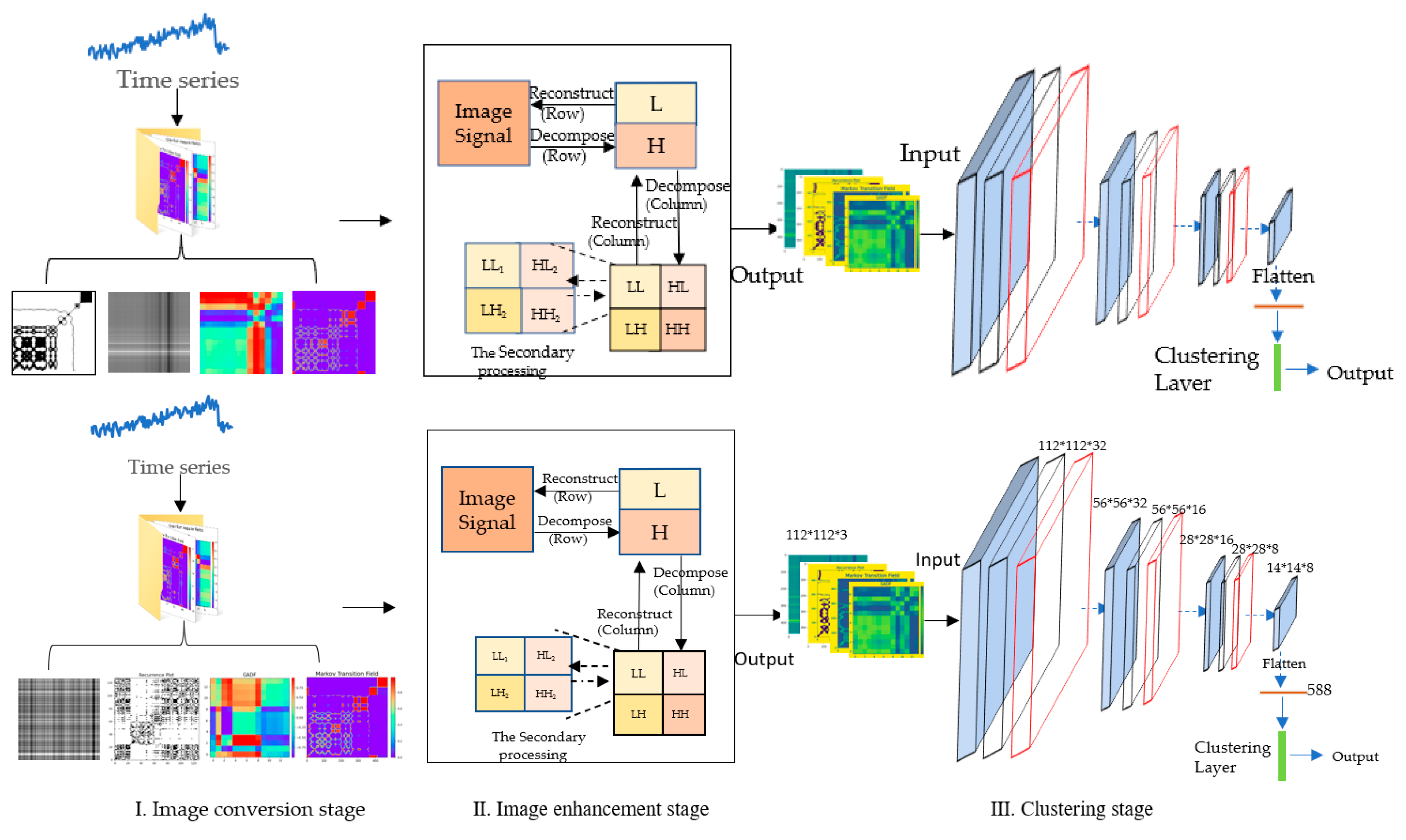
The proposed GW_DC model could convert the original time-series into two-dimensional images and then classify them into some groups. For comparison, time-series were converted into grayscale images, RP images, MTF images, and GADF images. Meanwhile, the deep clustering network was employed for classifying these enhanced two-dimensional images, and the convolution kernel factorization method was introduced into the DC network for reducing the number of parameters and improving the clustering performance. The frame of the proposed GW-DC model, depicted in Figure 1, consisted of three stages: the image conversion stage, image enhancement stage, and image clustering stage.
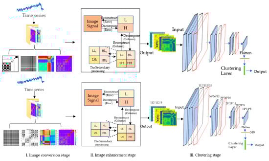
Figure 1.
The frame of the GW-DC model.
In the image conversion stage, the time-series was transformed into four kinds of two-dimensional images for expanding data volume and enhancing generalization ability, including grayscale images, RP images, MTF images, and GADF images. The low-dimensional features were mapped to a high-dimensional space for amplifying the feature attributes and improving the clustering effect. Through comparison, GADF with the best characterization effect was selected in this study.
In the image enhancement stage, the wavelet transform algorithm was used to enhance the texture features of the transformed two-dimensional images. The resolution of the images was regarded as the measurement standard of image decomposition, and the image signals were decomposed into high-frequency subband and low-frequency subband. The high-frequency subband was expanded, and the low-frequency subband was scaled for strengthening the change details of the time-series and enhancing the contrast ratio. Then, the processed signal components were reconstructed to obtain the enhanced images.
In the image clustering stage, a new deep clustering network DC was proposed to improve the clustering effect. In this stage, the DC network based on CNN was designed to learn and represent the features of two-dimensional images. Then, the obtained features were clustered by the K-Means algorithm, and the cross-entropy (CE) [27] was introduced as the loss function to optimize the DC network.
2.1. Image Conversion Stage
For well retaining the time correlation and frequency structure of the time-series, one-dimensional data were transformed into two-dimensional images. Time-series data were converted into four two-dimensional images, including grayscale images, RP images, MTF images, and GADF images. The clustering results according to different kinds of two-dimensional images were compared and analyzed to determine the best characterization effects of the aforementioned images. Four two-dimensional image representation methods were described in this section.
2.1.1. Conversion from Time-Series into Grayscale Image
The time-series of length could be expressed as . Then, for reducing the dimension of time-series, piecewise aggregation approximation (PAA) was adopted to compress time-series and a new smooth time-series curve was generated. The generated time-series could be expressed as , where is the length of time-series . The dimension of time-series was compressed into , with . The reduction factor is
where each row in the matrix contained every timestamp of the time-series, and each column was the transpose representation of the corresponding row for expanding the matrix data with redundancy features.
Then the data matrix was transformed into the gray value matrix (GVM), the corresponding gray value was obtained by using the maximum and minimum normalization method [28]. Six time-series datasets from the UCR website were applied to verify the performance of the model and visual display. The samples of four time-series datasets were converted into gray images. The visualization effect is shown in Figure 2.
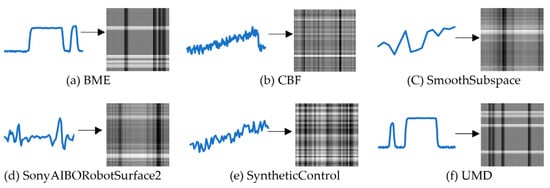
Figure 2.
The effect of converting six UCR datasets into the grayscale image.
The grayscale images intuitively present the general changes of different datasets. For example, the grayscale variation of the SonyAIBORobotSurface2 dataset is relatively flat, while the BME dataset shows a tendency to mutate.
2.1.2. Conversion from Time-Series into RP Images
RP was a time-time signal processing method that could be used to show the periodicity of trajectory in the phase space and reveal the internal structure of the time-series. It consisted of two-time axes, a black dot, and a white dot. The black dot indicated that recursion occurred in the state corresponding to the horizontal axis and vertical axis, and the white dot indicated that recursion did not occur. The key to constructing the RP image was to reconstruct the phase space, which needed to select the appropriate delay coefficient, embedding dimension, and threshold for reconstructing the time-domain information in the original phase space and promoting the signals to a higher dimension.
The transformation of the RP was divided into three steps, which were described as follows.
Step 1. For time-series , the sampling interval was determined to be . The appropriate embedding dimension was determined through relevant theoretical calculation, and the time-series was reconstructed. The reconstructed power system is
The length of time-series is
where is the length of time-series .
Step 2. The calculation of the distance between point and point in the reconstructed phase space is
where represents the L2 norm.
Step 3. The calculation of the recursive value is
where, is a square matrix with the size of , is equal to the vector numbers of , is the threshold, and represents the Heaviside function. The calculation of is
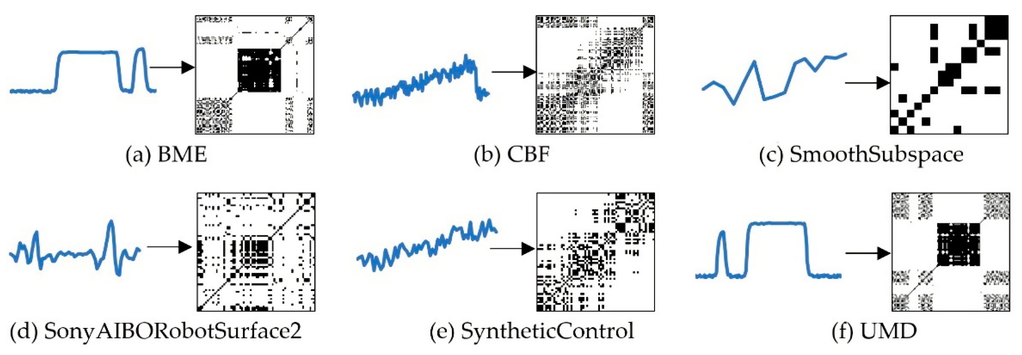
The effect of converting samples from different datasets into RP images is shown in Figure 3.
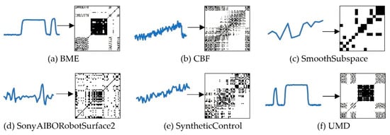
Figure 3.
The effect of converting time-series into Recurrence Plot.
The RP images clearly show the changes of different datasets through the arrangement of black and white blocks. For example, the SyntheticControl dataset generally presents a drift trend. The RP images of the UMD appear in large black areas and show a mutation mode, which is caused by the rapid change of data.
2.1.3. Conversion from Time-Series into MTF Images
The MTF method transformed one-dimensional time-series into two-dimensional images by constructing the discrete quantile of the Markov matrix and encoding the transition probability field. The MTF was obtained by adding the time position related to the first-order Markov chain. It provided an inverse operation to map the images back to the original signals, making the images easy to realize the visual representation.
The calculation process of the MTF could be divided into the following three steps.
Step 1. The data signals were discretized. First, the original time-series with length were divided into bins, and each data point belonged to a unique .
Step 2. The Markov transition matrix with the size of was constructed. was determined by the adjacent frequency of a point between two quantiles and , and its calculation formula is
Step 3. The time dependence was added to the transition probability matrix , and the Markov transition field with the size of was constructed. represents the transition probability from to , and the calculation of is
To better manage the graph and improve the operation efficiency, the principle of PAA was applied to this stage to reduce the size of the MTF matrix, and was gridded and averaged.
The effect of converting the time-series into MTF images is described in Figure 4.
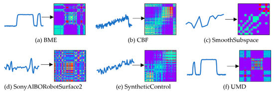
Figure 4.
The effect of converting the time-series into MTF images.
The MTF images intuitively show the change law through the variation of colors. And the trends in MTF images are similar to grayscale images and RP images.
2.1.4. Conversion from Time-Series to Gramian Angular Difference Field
The Gramian Angular Field (GAF) method was used to transform the scaled one-dimensional time-series into a polar coordinate system and construct the objective mapping between one-dimensional time-series and two-dimensional space. Then, the GAF method could be divided into two implementation methods according to the calculation angle between different time points, including Gramian Angular Summation Field (GASF) and GADF. A GAF image was a graphical representation of a Gramian matrix in which each element was the superposition of directions between different time intervals, and the polar coordinate system was used to retain the time correlation.
The conversion processes of GASF and GADF were similar, and the conversion process of GADF was as follows.
Step 1. One-dimensional time-series were scaled numerically. The time-series in the Cartesian coordinate system was scaled to interval and the calculation of time series scaling is
Step 2. The scaled sequence data were transformed from a Cartesian coordinate system to a polar coordinate system in which the value was regarded as the cosine of the included angle, the timestamp was treated as the radius, and the function was used for mapping. This method retained the time dependence through the coordinate, and the coordinate transformation equations is
where, is the time stamp, and is a constant factor to regularize the span of the polar coordinate system.
Step 3. The GADF matrix was obtained by the trigonometric function transformation of two angular differences. The calculation of the GADF matrix is
Similar to other image characterization methods mentioned earlier, the PAA method was used to retain the sequence trend and reduce the sequence size at this stage.
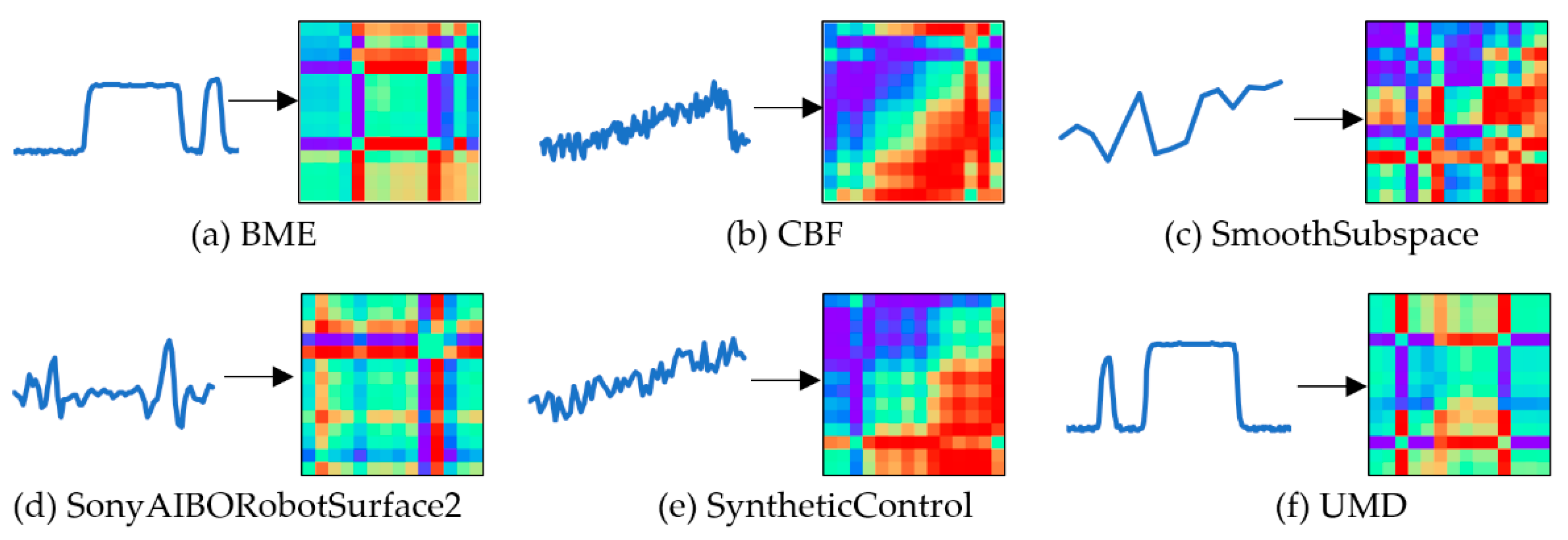
The effect of converting the time-series into GADF images is described in Figure 5.

Figure 5.
The effect of converting the time-series into GADF images.
The GADF images reveal the temporal correlation between data pairs and preserve the spatial variation law intuitively. And the variation in GADF images is roughly the same as that of the abovementioned three image representation methods.
2.2. Image Enhancement Stage
The multi-resolution decomposition of wavelet transform was used to perform multistage two-dimensional discrete wavelet transform on the images by low-pass and high-pass filters. Then, the image signals were decomposed into low-frequency and high-frequency components. In the images, most of the noise and some edge details belonged to the high-frequency subband, while the low-frequency subband was mainly characterized as the approximate signals of the images. The high-frequency and low-frequency subband were processed by different methods to enhance the images, including reducing noise, improving contrast, and strengthening details. Then, the reconstructed image was obtained by inverse discrete wavelet transform on the processed components.
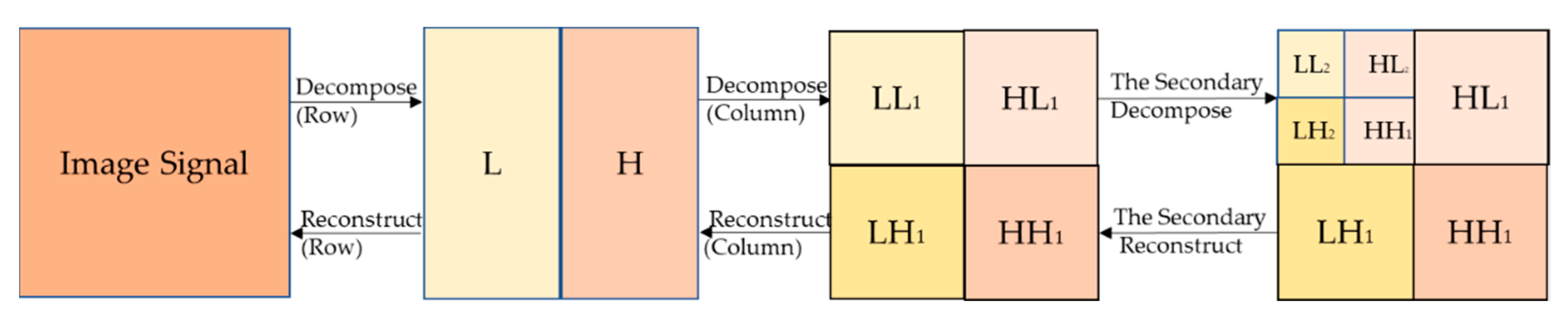
The two-dimensional image signals were filtered in horizontal and vertical directions for realizing the two-dimensional wavelet multi-resolution decomposition. First, the signals of the images were decomposed according to the line for obtaining the low-frequency component and high-frequency component in the horizontal direction. Then, the columns of the transformed data were decomposed to obtain the low-frequency components ) and high-frequency components in four directions. The reconstructed images could be obtained by inverse discrete wavelet transform in the opposite direction. The aforementioned process of image decomposition and reconstruction is described in Figure 6.
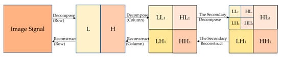
Figure 6.
The frame of the RPM-K-Means model.
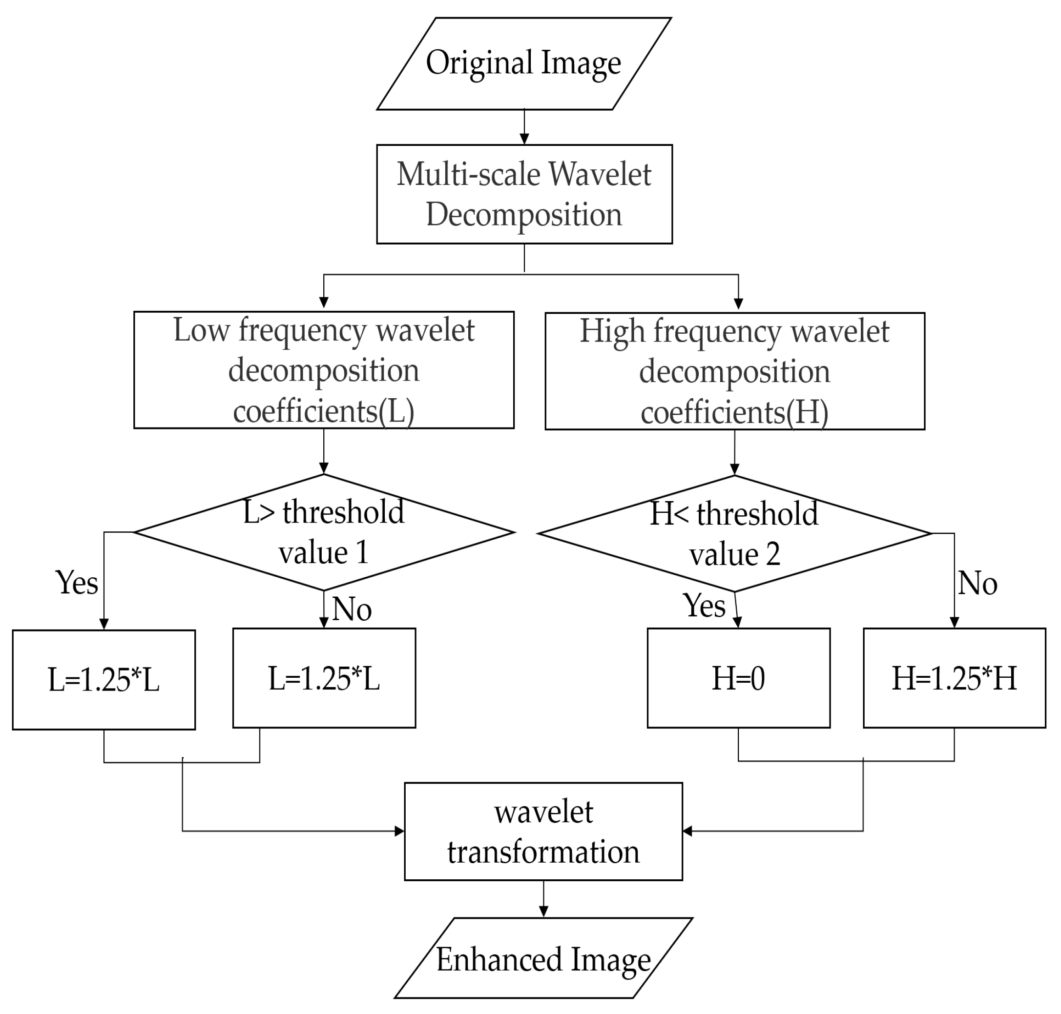
The subband was an approximate representation obtained using a low-pass wavelet filter. The subband was obtained using a low-pass wavelet filter and a high-pass wavelet filter, which showed the singularity of the image in the horizontal direction. The subband was obtained using the aforementioned two filters and represented the singular characteristics of the image in the vertical direction. The subband, obtained using a high-pass wavelet filter, indicated the diagonal edge characteristics of the images. Different measures were taken for the low-frequency and high-frequency components to improve the contrast of the images and strengthen the texture details in the images. If the low-frequency coefficient was greater than 250, it was multiplied by 0.75. If the high-frequency coefficient was less than 150, it was multiplied by 1.25. The aforementioned process is depicted in Figure 7.
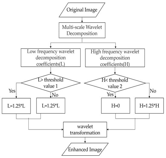
Figure 7.
The processes of the wavelet transform.
2.3. Image Clustering Stage
In this stage, an unsupervised deep clustering network DC was designed and applied. The target of the DC network was to define a parametric nonlinear mapping from the data space to the low-dimensional feature space, and complete clustering in the low-dimensional space. Following the idea of the DEC model and the inception network, a deep clustering network DC was designed. The DC included an improved autoencoder for feature learning and a clustering layer for clustering.
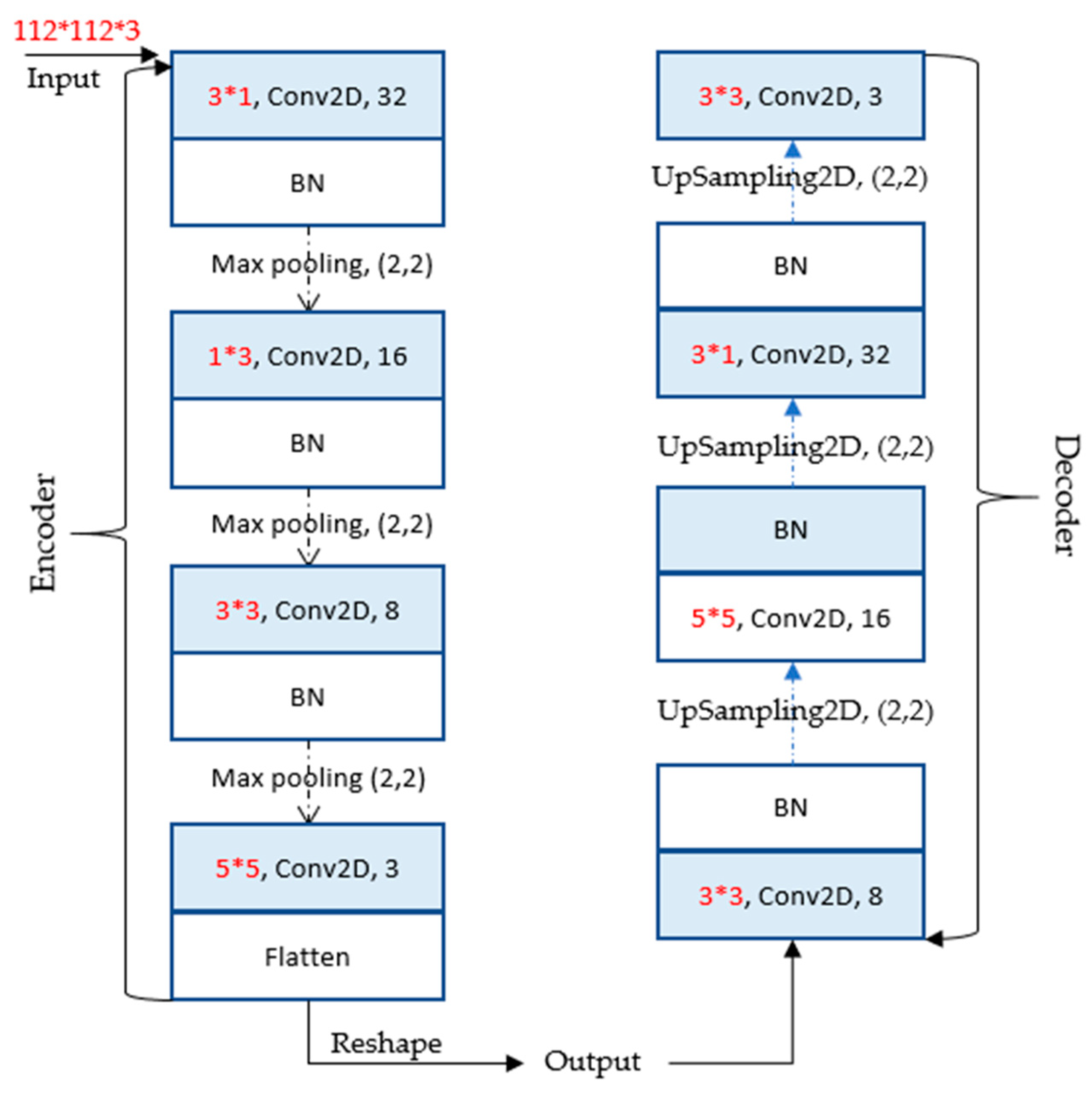
In the feature learning stage, the autoencoder-incorporated convolution kernel factorization method was trained to learn the mapping parameters from the data space to the feature space. The asymmetric convolution kernel factorization was first proposed by Szegedy [29] and its application effect in the CNN network was demonstrated. According to the convolution kernel factorization, the convolution kernel of 3 ∗ 3 was replaced by 1 ∗ 3 and 3 ∗ 1 for reducing the number of parameters, and the obtained receptive field was not reduced. Meanwhile, the symmetric structure of samples was obtained after enhancement, and the model could learn more valuable representations. The structural parameters of the improved autoencoder are shown in Figure 8.
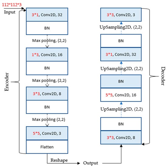
Figure 8.
The network of the autoencoder.
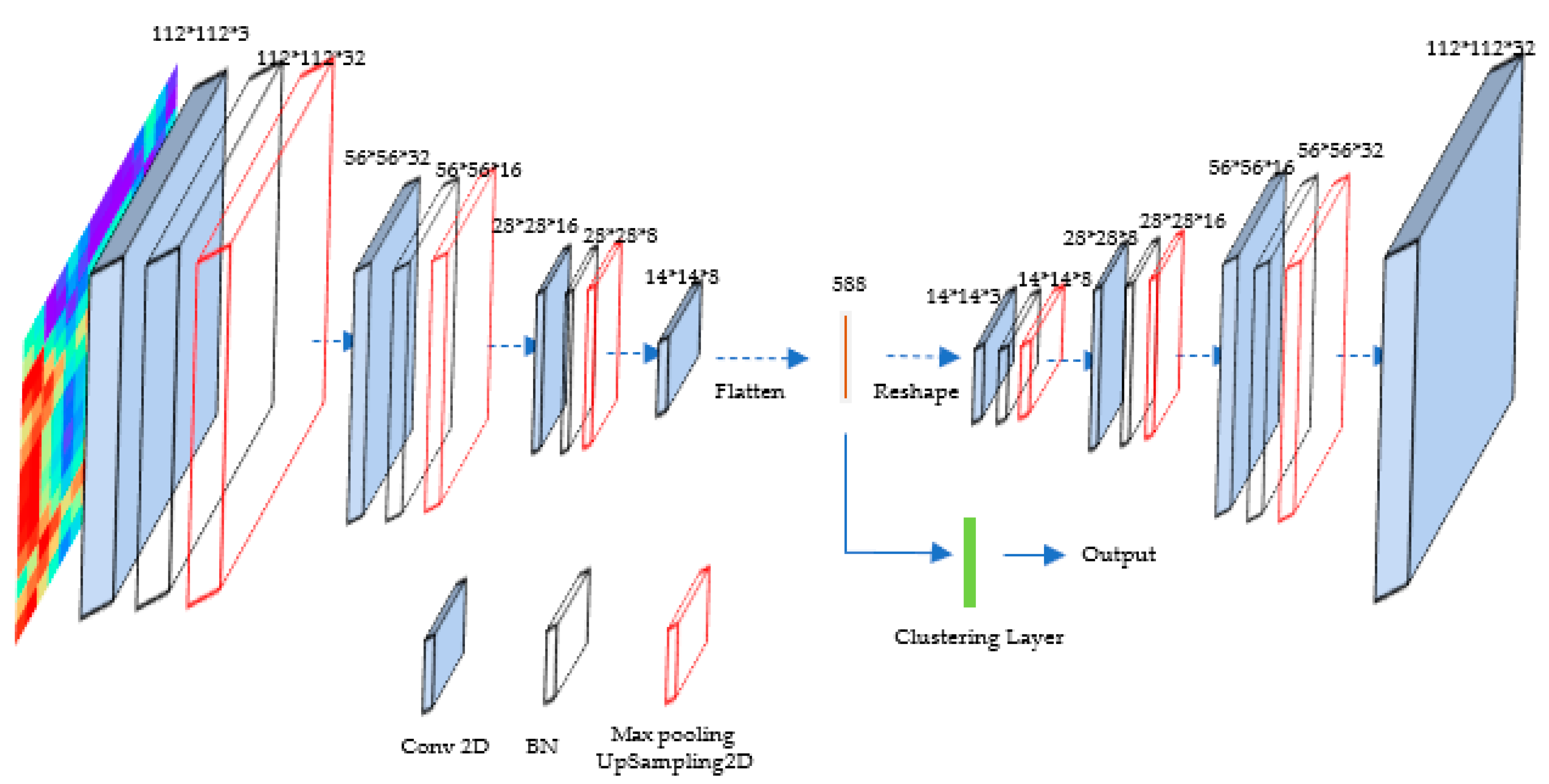
The improved autoencoder consisted of an encoder and a decoder. The encoder stored the parameters of the learned feature representation, and the decoder was employed to reconstruct the data. The encoder was composed of 10 layers, and the number of its channels was 3, 32, 32, 32, 16, 16, 16, 8, 8, and 8, respectively. The small 3 ∗ 1 receptive field was set in the first convolution layer, followed by the second convolution layer with a 1 ∗ 3 effective receptive field. Then, the convolution kernels of 3 ∗ 3 and 5 ∗ 5 were subsequently added to obtain comprehensive distinctive features. The first three convolution layers were followed by batch normalization (BN) and max pooling. The flattening operation for learned feature representation was performed at the end of the encoder. The decoder consisted of 10 layers, and the number of its channels was 3, 8, 8, 8, 16, 16, 16, 32, 32, and 32, respectively. The decoder network contained four convolution layers with weight, as shown in Figure 8. The first three convolution layers of the decoder were followed by BN and upsampling operation. Relu non-linearity was applied to every convolution layer. Then, the numerical probability of the predicted output was mapped to [0, 1]. The process of the DC is depicted in Figure 9.

Figure 9.
The structure of the proposed DC.
After pre-training, the decoder layers were discarded and the encoder was employed as the initial mapping between the data space and the feature space. The output of the encoder was used as the input of the clustering layer, and the feature data were clustered using the K-Means algorithm. Meanwhile, the CE was cited as the loss function to optimize the objective function. The loss function is
where, represents the real label, denotes the predicted probability that the current sample label is 1, and is the predicted probability that the current sample label is 0. is the total loss function of n samples and represents the difference between the ground truth and predicted values.
3. Experiment and Results
3.1. Datasets and Evaluation Index
To verify the performance of the proposed model, six time-series datasets shown in Table 1 were adopted from the UCR time-series website. The length of these datasets ranged from 150 to 15, and the classes of these datasets ranged from 2 to 6. The values of these datasets were normalized using Equation (11) for clustering analysis. The training and test sets of each dataset were provided directly by the UCR time-series website. The specific descriptions of the six datasets are shown in Table 1.

Table 1.
Description of datasets.
To evaluate the clustering effect of the proposed GW-DC model, normalized mutual information (NMI) [30] and unsupervised clustering accuracy (ACC) were employed to measure the clustering results. Hence, NMI was selected to measure the similarity in different data distributions, and its calculation formula is
where mutual information represents the variation of the clustering information , given the class information . represents the entropy, and . The greater the value of NMI, the greater the correlation between data and classes.
The mutual information of clustering is
where is the probability that the sample belongs to both class and class . represents the probability that the sample belongs to the class , and is similar to . The greater the value of mutual information, the greater the degree of correlation between the data and the category.
The calculation of ACC is
where, and represent the real label and the predicted label of sample respectively. denotes all possible one-to-one mappings between clusters and labels.
3.2. Conversion Result of Two-Dimensional Images
The time-series were converted into four kinds of two-dimensional images, including grayscale images, RP images, MTF images, and GADF images. The clustering results of the next stage were used to determine the best image feature representation method. The six public datasets were converted into four kinds of two-dimensional images, and wavelet transform was applied to enhance the obtained images. Then, the proposed DC network was used to cluster according to the enhanced images. The clustering index NMI (%) is shown in Table 2.
Table 2.
The clustering results according to four kinds of images.
The CBF and SonyAIBORobotSurface2 datasets had the best clustering results according to the RP images, only 4% and 2% higher than that for GADF images, respectively. The BME dataset had the best clustering effect according to the grayscale images and GADF images, and their results were 91.18%. The other datasets had the best clustering results according to GADF images. Comprehensively, the GADF representation method had a better representation effect, and this method was selected for image feature representation.
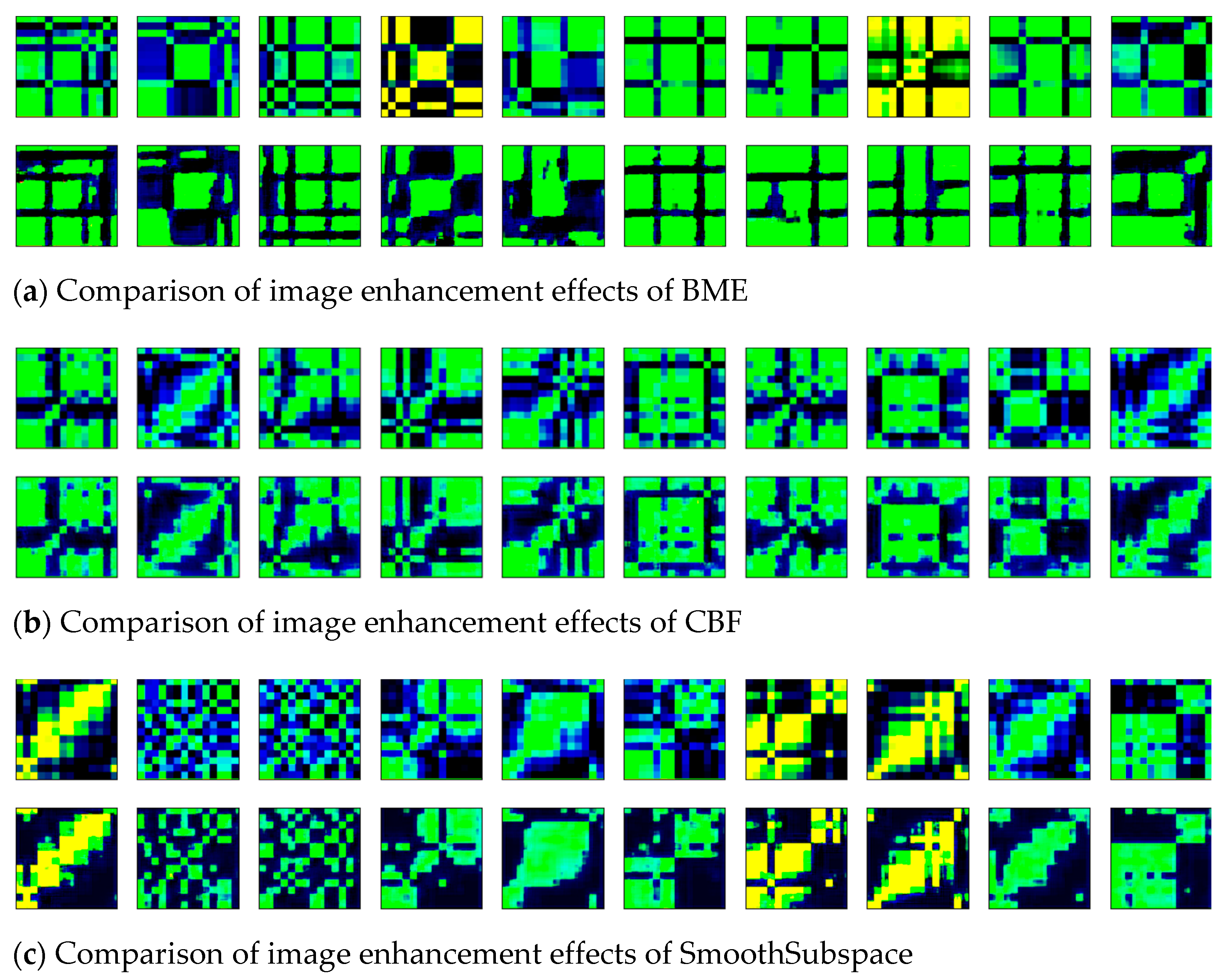
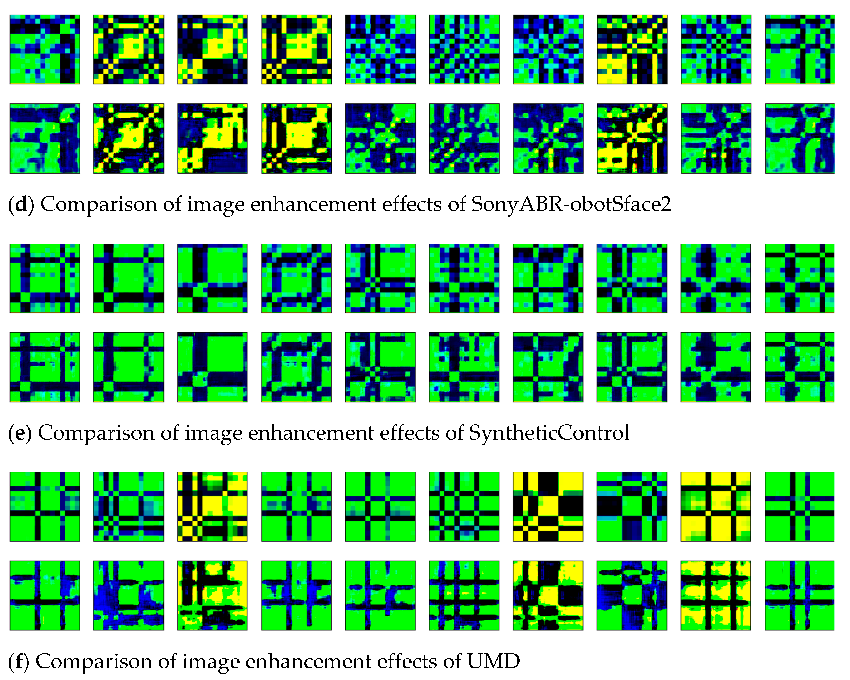
The time-series of six datasets were transformed into two-dimensional images by the GADF, and the obtained images were denoised and enhanced by the wavelet transform method. To visualize the effect of image enhancement, the original two-dimensional images (shown in Line 1) and the enhanced images (shown in Line 2) of six datasets were displayed, as shown in Figure 10a–f.
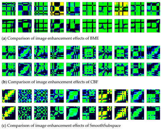
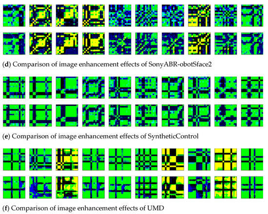
Figure 10.
The comparison of image enhancement effects of six datasets.
Ten images in each dataset were randomly selected for comparative display. In the enhanced images, the blurred noise points were reduced, and the contour edge was clearer than the original images. The texture features of the images were enhanced by the wavelet transform method.
3.3. Comparative Analysis of Clustering Results
To verify the robustness of the proposed model, the clustering results of the GW-DC were compared with those of five other clustering models, including Stacked Autoencoder (SAE) +K-Means, Autoencoder (AE) +K-Means, AE_Conv +K-Means, DEC, and DEC_FCN. AE_Conv +K-Means was the structure that replaced the fully connected layer (FCL) in AE with the convolutional layer. DEC_FCN referred to the structure that replaced the convolutional layer in DEC models with FCLS. The index NMI (%) and ACC (%) were employed to measure the clustering effect. The comparative results of different models are shown in Table 3.
Table 3.
Results of different deep clustering models.
Compared with the AE +K-Means model, the NMI and clustering accuracy of the AE_Conv +K-Means model on five datasets were improved, and the maximum difference in NMI and accuracy were 13.15% and 24.17%, respectively. Comparing the results of the DEC and the DEC_FCN, the DEC model with convolutional layers displayed a better clustering effect. Besides, the SonyAIBORobotSurface2 dataset had a higher clustering effect on the DEC model with NMI and accuracy of 30.17% and 79.08%, respectively. In the other five datasets, the NMI index of the GW-DC model was significantly higher than that of DEC, and the maximum difference reached 44.49%. Through comparative analysis of clustering indexes, the GW-DC model showed a better clustering effect than that of other deep clustering models.
4. Conclusions
To solve the problem of low clustering accuracy and difficulty in expanding to large datasets, we proposed to convert time-series datasets into two-dimensional images and designed a deep clustering network to improve the effect of unsupervised clustering. Through comparative analysis, the GADF images showed the best characterization effect among the four image representation methods. This method could map the low-dimensional data to the high-dimensional space for revealing the time correlation of the data. Therefore, the main contributions in this study were the integration of the GADF transformation method and wavelet transform as well as the design of the DC network for clustering according to enhanced two-dimensional images. The wavelet transform method, applied in the image enhancement stage, could enhance the texture features of two-dimensional images and enlarge the relevant attributes of the data (Figure 10). Then, in the clustering stage, the DC network based on CNN was designed and used to learn the characteristics of images, and the K-Means algorithm was applied for unsupervised clustering. The convolution kernel factorization method was introduced to reduce the amount of parameter calculation and improve clustering performance. The CE was cited as the loss function to optimize the objective function. Through experimental analysis, the proposed GW-DC model showed a better clustering effect than other models; the comparison result is described in Section 3.3, and the maximum difference in NMI reached 44.49%.
Author Contributions
Conceptualization, T.L., X.L. and Y.W.; data curation, Y.W.; formal analysis, T.L.; funding acquisition, T.L.; investigation, Y.W.; methodology, X.L. and Y.W.; project administration, T.L.; resources, Y.W.; supervision, T.L.; validation, X.L. and Y.W.; visualization, Y.W.; writing–original draft, T.L. and Y.W.; writing–review and editing, T.L. and Y.W. All authors have read and agreed to the published version of the manuscript.
Funding
This research is funded by the National Natural Science Foundation of China, grant number 51939001, and 61976033, the National Social Science Foundation of China, grant number 15CGL031, Young Foundation of Ministry of Education Humanities and Social Sciences, grant number 21YJC630066, the Liaoning Revitalization Talents Program, grant number XLYC1907084, the Science & Technology Innovation Funds of Dalian, grant number 2018J11CY022, the Fundamental Research Funds for the Central Universities, grant number 3132019353 and 3132021273.
Institutional Review Board Statement
Not applicable.
Informed Consent Statement
Not applicable.
Data Availability Statement
Not applicable.
Conflicts of Interest
The authors declare no conflict of interest.
References
- Li, H.L. Multivariate time series clustering based on common principal component analysis. Neurocomputing 2019, 349, 239–247. [Google Scholar] [CrossRef]
- Chira, C.; Sedano, J.; Camara, M.; Prieto, C.; Villar, J.R.; Corchado, E. A cluster merging method for time series microarray with production values. Int. J. Neural Syst. 2014, 24, 1450018. [Google Scholar] [CrossRef] [PubMed]
- Karim, F.; Majumdar, S.; Darabi, H.; Chen, S. LSTM fully convolutional networks for time series classification. IEEE Access 2018, 6, 1662–1669. [Google Scholar] [CrossRef]
- Gao, Y.P.; Chang, D.F.; Fang, T.; Fan, Y.Q. The Daily Container Volumes Prediction of Storage Yard in Port with Long Short-Term Memory Recurrent Neural Network. Available online: https://www.hindawi.com/journals/jat/2019/5764602/ (accessed on 15 November 2021).
- Li, H.T.; Bai, J.C.; Li, Y.W. A novel secondary decomposition learning paradigm with kernel extreme learning machine for multi-step forecasting of container throughput. Physica A 2019, 534, 122025. [Google Scholar] [CrossRef]
- Liao, T.W. Clustering of time series data—A survey. Pattern Recognit. 2005, 38, 1857–1874. [Google Scholar] [CrossRef]
- Huang, X.H.; Ye, Y.M.; Xiong, L.Y.; Lau, R.Y.K.; Jiang, N.; Wang, S.K. Time series k-means: A new k-means type smooth subspace clustering for time series data. Inf. Sci. 2016, 367, 1–13. [Google Scholar] [CrossRef]
- Guijo-Rubio, D.; Duran-Rosal, A.M.; Gutierrez, P.A.; Troncoso, A.; Hervas-Martinez, C. Time-Series Clustering Based on the Characterization of Segment Typologies. IEEE Trans. Cybern. 2020, 51, 2962584. [Google Scholar] [CrossRef]
- Zhang, Y.P.; Qu, H.; Wang, W.P.; Zhao, J.H. A Novel Fuzzy Time Series Forecasting Model Based on Multiple Linear Regression and Time Series Clustering. Available online: https://www.hindawi.com/journals/mpe/2020/9546792/ (accessed on 15 November 2021).
- Hung, W.L.; Yang, M.S. Similarity measures of intuitionistic fuzzy sets based on Hausdorff distance. Pattern Recognit. Lett. 2004, 25, 1603–1611. [Google Scholar] [CrossRef]
- Xu, H.; Zeng, W.H.; Zeng, X.X.; Yen, G.G. An evolutionary algorithm based on Minkowski distance for many-objective optimization. IEEE T. Cybern. 2019, 49, 3968–3979. [Google Scholar] [CrossRef]
- Ioannidou, Z.S.; Theodoropoulou, M.C.; Papandreou, N.C.; Willis, J.H.; Hamodrakas, S.J. CutProtFam-Pred: Detection and classification of putative structural cuticular proteins from sequence alone, based on profile hidden Markov models. Insect Biochem. Mol. Biol. 2014, 52, 51–59. [Google Scholar] [CrossRef] [Green Version]
- Liu, H.C.; Liu, L.; Li, P. Failure mode and effects analysis using intuitionistic fuzzy hybrid weighted Euclidean distance operator. Int. J. Syst. Sci. 2014, 45, 2012–2030. [Google Scholar] [CrossRef]
- Guan, X.D.; Huang, C.; Liu, G.H.; Meng, X.L.; Liu, Q.S. Mapping rice cropping systems in Vietnam using an NDVI-based time-series similarity measurement based on DTW distance. Remote Sens. 2016, 8, 19. [Google Scholar] [CrossRef] [Green Version]
- Wang, J.; Wu, J.; Ni, J.; Chen, J.; Xi, C. Relationship between Urban Road Traffic Characteristics and Road Grade Based on a Time Series Clustering Model: A Case Study in Nanjing, China. Chin. Geogr. Sci. 2018, 28, 1048–1060. [Google Scholar] [CrossRef] [Green Version]
- Yang, B.; Fu, X.; Sidiropoulos, N.D.; Hong, M.Y. Towards K-means-friendly Spaces: Simultaneous Deep Learning and Clustering. In Proceedings of the 34th International Conference on Machine Learning (ICML), Sydney, Australia, 6–11 August 2017. [Google Scholar]
- Huang, P.H.; Huang, Y.; Wang, W.; Wang, L. Deep Embedding Network for Clustering. In Proceedings of the 22nd International Conference on Pattern Recognition (ICPR), Stockholm, Sweden, 24–28 August 2014. [Google Scholar]
- Ji, P.; Zhang, T.; Li, H.D.; Salzmann, M.; Reid, I. Deep subspace clustering networks. In Proceedings of the 31st Annual Conference on Neural Information Processing Systems (NIPS), Long Beach, CA, USA, 4–9 December 2017. [Google Scholar]
- Chen, D.; Lv, J.C.; Yi, Z. Unsupervised multi-manifold clustering by learning deep representation. In Proceedings of the 31st AAAI Conference on Artificial Intelligence (AAAI), San Francisco, CA, USA, 4–9 February 2017. [Google Scholar]
- Lee, H.; Grosse, R.; Ranganath, R.; Ng, A.Y. Convolutional deep belief networks for scalable unsupervised learning of hierarchical representations. In Proceedings of the 26th Annual International Conference on Machine Learning, Montreal, ON, Canada, 14–18 June 2009. [Google Scholar]
- Chen, J. Deep Learning with Nonparametric Clustering. arXiv 2015, arXiv:1501.03084. Available online: https://arxiv.org/abs/1501.03084 (accessed on 15 November 2021).
- Xie, J.; Girshick, R.; Farhadi, A. Unsupervised Deep Embedding for Clustering Analysis. arXiv 2016, arXiv:1511.06335. Available online: https://arxiv.org/abs/1511.06335 (accessed on 15 November 2021).
- Li, F.F.; Qiao, H.; Zhang, B. Discriminatively boosted image clustering with fully convolutional auto-encoders. Pattern Recognit. 2018, 83, 161–173. [Google Scholar] [CrossRef] [Green Version]
- Goodfellow, I.J.; Pouget-Abadie, J.; Mirza, M.; Xu, B.; Warde-Farley, D.; Ozair, S.; Courville, A.; Bengio, Y. Generative adversarial nets. Adv. Neural Inf. Process. Syst. 2014, 27, 2672–2680. [Google Scholar]
- Jiang, Z.; Zheng, Y.; Tan, H.; Tang, B.; Zhou, H. Variational Deep Embedding: An Unsupervised and Generative Approach to Clustering. arXiv 2016, arXiv:1611.05148. Available online: https://arxiv.org/abs/1611.05148 (accessed on 15 November 2021).
- Chang, J.; Wang, L.; Meng, G.; Xiang, S.; Pan, C. Deep adaptive image clustering. In Proceedings of the 2017 IEEE International Conference on Computer Vision (ICCV), Venice, Italy, 22–29 October 2017. [Google Scholar]
- Liu, L.Z.; Qian, X.Y.; Lu, H.Y. Cross-sample entropy of foreign exchange time series. Physica A 2010, 389, 4785–4792. [Google Scholar] [CrossRef]
- Chen, W.; Shi, K. A deep learning framework for time series classification using Relative Position Matrix and Convolutional Neural Network. Neurocomputing 2019, 359, 384–394. [Google Scholar] [CrossRef]
- Szegedy, C.; Vanhoucke, V.; Loffe, S.; Shlens, J.; Wojna, Z. Rethinking the Inception Architecture for Computer Vision. In Proceedings of the 2016 IEEE Conference on Computer Vision and Pattern Recognition (CVPR), Las Vegas, NV, USA, 27–30 June 2016. [Google Scholar]
- Contreras-Reyes, J.E. Mutual information matrix based on asymmetric Shannon entropy for nonlinear interactions of time series. Nonlinear Dyn. 2021, 104, 3913–3924. [Google Scholar] [CrossRef]
- Tian, F.; Gao, B.; Cui, Q.; Chen, E.H.; Liu, T.Y. Learning Deep Representations for Graph Clustering. In Proceedings of the 28th AAAI Conference on Artificial Intelligence (AAAI), Quebec City, QC, Canada, 27–31 July 2014. [Google Scholar]
- Song, C.F.; Liu, F.; Huang, Y.Z.; Wang, L.; Tan, T.N. Auto-Encoder Based Data Clustering; Springer: Berlin/Heidelberg, Germany, 2013. [Google Scholar]


Publisher’s Note: MDPI stays neutral with regard to jurisdictional claims in published maps and institutional affiliations. |
© 2021 by the authors. Licensee MDPI, Basel, Switzerland. This article is an open access article distributed under the terms and conditions of the Creative Commons Attribution (CC BY) license (https://creativecommons.org/licenses/by/4.0/).