
Forecast of Medical Costs in Health Companies Using Models Based on Advanced Analytics

 , , ,
, , ,  and
and
Abstract
:1. Introduction
2. Related Work
3. Materials and Methods
3.1. Data Collection
3.2. Data Processing
- Dates are converted into DateTime Y%–M%–D% and thus dates are formatted;
- Empty fields of dates are denoted by 1900–01–01;
- Empty fields are mapped in 0 values;
- The “TotalComorbidities” field is created, allowing to identify the number of diagnoses or cohorts of a patient;
- Category values are encoded;
- Mappings to a dictionary of types of documents;
- Exceedingly small provision values of less than 1000 are disregarded;
- DateTime Y%–M%–D% dates are formatted;
- The “Number” and “InvoicedValue” fields are converted into int. format.
3.3. Model Implementation
3.3.1. LSTM Networks
model.add(LSTM(2))
model.add(Dropout(0.2))
model.add(Dense(1))
model.compile(optimizer=‘adam’, loss=‘mean_squared_error’)
model.fit(batch_size=1, verbose=0, epochs = 20, shuffle = False)
3.3.2. Clusters
4. Results
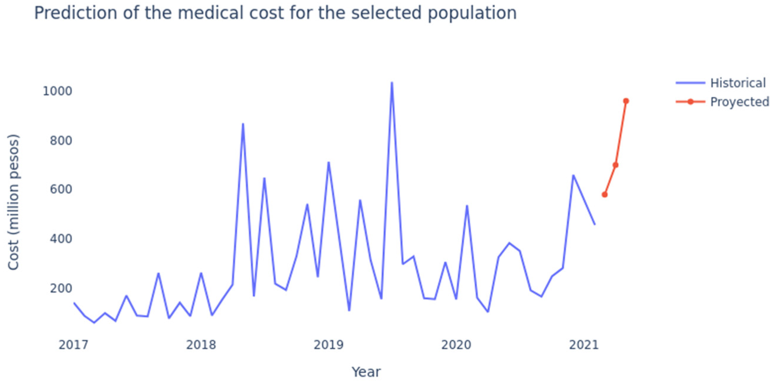
4.1. LSTM Networks
4.2. Clustering
4.2.1. Distribution by Age Cluster (in Years)
4.2.2. Distribution by Frequency of Use Cluster
4.2.3. Distribution by Cluster of Last Attention Time (Recency)
4.2.4. Distribution by Cluster of Weeks Contributed since Last Year
4.2.5. Distribution by Cluster of Continuous Contributed Weeks
5. Discussion
6. Conclusions
Author Contributions
Funding
Institutional Review Board Statement
Informed Consent Statement
Data Availability Statement
Conflicts of Interest
Appendix A

| Cluster | R2 | Adj. R2 |
|---|---|---|
| 0 | 0.91 | 0.87 |
| 1 | 0.95 | 0.91 |
| 2 | 0.92 | 0.82 |
| 3 | 0.98 | 0.92 |
| 4 | 0.97 | 0.96 |
References
- Yang, C.; Delcher, C.; Shenkman, E.; Ranka, S. Machine Learning Approaches for Predicting High Utilizers in Health Care. In Proceedings of the International Conference on Bioinformatics and Biomedical Engineering, Granada, Spain, 26–28 April 2017; Lecture Notes in Computer Science (Including Subseries Lecture Notes in Artificial Intelligence and Lecture Notes in Bioinformatics). Springer: Cham, Switzerland, 2017; Volume 10209 LNCS, pp. 382–395. [Google Scholar]
- Current Health Expenditure (CHE) as Percentage of Gross Domestic Product (GDP) (%). Available online: https://www.who.int/data/gho/data/indicators/indicator-details/GHO/current-health-expenditure-(che)-as-percentage-of-gross-domestic-product-(gdp)-(-) (accessed on 19 January 2022).
- Morid, M.A.; Sheng, O.R.L.; Kawamoto, K.; Ault, T.; Dorius, J.; Abdelrahman, S. Healthcare Cost Prediction: Leveraging Fine-Grain Temporal Patterns. J. Biomed. Inform. 2019, 91, 103113. [Google Scholar] [CrossRef] [PubMed]
- Sushmita, S.; Newman, S.; Marquardt, J.; Ram, P.; Prasad, V.; de Cock, M.; Teredesai, A. Population Cost Prediction on Public Healthcare Datasets. In Proceedings of the 5th International Conference on Digital Health 2015, Florence, Italy, 18–20 May 2015; ACM International Conference Proceeding Series. Association for Computing Machinery: New York, NY, USA, 2015; Volume 2015, pp. 87–94. [Google Scholar]
- Ministerio de Salud y Protección Social $31.8 Billones Para La Salud En 2020. Available online: https://www.minsalud.gov.co/Paginas/31-8-billones-para-la-salud-en-2020.aspx (accessed on 4 January 2022).
- El Presupuesto de La Nación de 2021 Destinará $75 Billones Para Deuda, 6.7% Del PIB. Available online: https://www.larepublica.co/economia/presupuesto-de-la-nacion-de-2021-destinara-75-billones-para-deuda-67-del-pib-3038167 (accessed on 5 January 2022).
- About Keralty—Keralty. Available online: https://www.keralty.com/en/web/guest/about-keralty (accessed on 3 May 2021).
- Giedion, U.; Díaz, B.Y.; Alfonso, E.A.; Savedoff, W.D. The Impact of Subsidized Health Insurance on Access, Utilization and Health Status in Colombia. Utilization and Health Status in Colombia (May 2007). iHEA 2007 6th World Congress: Explorations in Health Economics Paper. 2007, p. 199. Available online: https://www.researchgate.net/publication/228233420_The_Impact_of_Subsidized_Health_Insurance_on_Access_Utilization_and_Health_Status_in_Colombia (accessed on 4 February 2022).
- Plan Obligatorio de Salud. Available online: https://www.minsalud.gov.co/proteccionsocial/Paginas/pos.aspx (accessed on 8 January 2022).
- Paho—Health in the Americas—Colombia. Available online: https://www.paho.org/salud-en-las-americas-2017/?p=2342 (accessed on 3 May 2021).
- Hochreiter, S.; Schmidhuber, J. Long Short-Term Memory. Neural Comput. 1997, 9, 1735–1780. [Google Scholar] [CrossRef] [PubMed]
- Kaushik, S.; Choudhury, A.; Dasgupta, N.; Natarajan, S.; Pickett, L.A.; Dutt, V. Using LSTMs for Predicting Patient’s Expenditure on Medications. In Proceedings of the 2017 International Conference on Machine Learning and Data Science (MLDS 2017), Noida, India, 14–15 December 2017; pp. 120–127. [Google Scholar] [CrossRef]
- Graves, A. Generating Sequences with Recurrent Neural Networks. arXiv 2013, arXiv:1308.0850. [Google Scholar]
- Tu, L.; Lv, Y.; Zhang, Y.; Cao, X. Logistics Service Provider Selection Decision Making for Healthcare Industry Based on a Novel Weighted Density-Based Hierarchical Clustering. Adv. Eng. Inform. 2021, 48, 101301. [Google Scholar] [CrossRef]
- Zhang, Z.; Murtagh, F.; van Poucke, S.; Lin, S.; Lan, P. Hierarchical Cluster Analysis in Clinical Research with Heterogeneous Study Population: Highlighting Its Visualization with R. Ann. Transl. Med. 2017, 5, 75. [Google Scholar] [CrossRef] [PubMed] [Green Version]
- Abbi, R.; El-Darzi, E.; Vasilakis, C.; Millard, P. A Gaussian Mixture Model Approach to Grouping Patients According to Their Hospital Length of Stay. In Proceedings of the 2008 21st IEEE International Symposium on Computer-Based Medical Systems, Jyvaskyla, Finland, 17–19 June 2008; pp. 524–529. [Google Scholar] [CrossRef]
- Santos, A.M.; de Carvalho Filho, A.O.; Silva, A.C.; de Paiva, A.C.; Nunes, R.A.; Gattass, M. Automatic Detection of Small Lung Nodules in 3D CT Data Using Gaussian Mixture Models, Tsallis Entropy and SVM. Eng. Appl. Artif. Intell. 2014, 36, 27–39. [Google Scholar] [CrossRef]
- 2.3. Clustering—Scikit-Learn 1.0.2 Documentation. Available online: https://scikit-learn.org/stable/modules/clustering.html (accessed on 24 January 2022).
- Implementing a K-Means Clustering Algorithm from Scratch|by Zack Murray|the Startup|Medium. Available online: https://medium.com/swlh/implementing-a-k-means-clustering-algorithm-from-scratch-214a417b7fee (accessed on 8 January 2022).
- K-Means Clustering: Algorithm, Applications, Evaluation Methods, and Drawbacks|by Imad Dabbura|towards Data Science. Available online: https://towardsdatascience.com/k-means-clustering-algorithm-applications-evaluation-methods-and-drawbacks-aa03e644b48a (accessed on 8 January 2022).
- Fontalvo-Herrera, T.; Delahoz-Dominguez, E.; Fontalvo, O. Methodology of Classification, Forecast and Prediction of Healthcare Providers Accredited in High Quality in Colombia. Int. J. Product. Qual. Manag. 2021, 33, 1–20. [Google Scholar] [CrossRef]
- Kaushik, S.; Choudhury, A.; Sheron, P.K.; Dasgupta, N.; Natarajan, S.; Pickett, L.A.; Dutt, V. AI in Healthcare: Time-Series Forecasting Using Statistical, Neural, and Ensemble Architectures. Front. Big Data 2020, 3, 4. [Google Scholar] [CrossRef] [Green Version]
- Kabir, S.B.; Shuvo, S.S.; Ahmed, H.U. Use of Machine Learning for Long Term Planning and Cost Minimization in Healthcare Management. medRxiv 2021. [Google Scholar] [CrossRef]
- Scheuer, C.; Boot, E.; Carse, N.; Clardy, A.; Gallagher, J.; Heck, S.; Marron, S.; Martinez-Alvarez, L.; Masarykova, D.; Mcmillan, P.; et al. Predicting Utilization of Healthcare Services from Individual Disease Trajectories Using RNNs with Multi-Headed Attention. Proc. Mach. Learn. Res. 2020, 116, 93–111. [Google Scholar] [CrossRef]
- Elbattah, M.; Molloy, O. Data-Driven Patient Segmentation Using K-Means Clustering: The Case of Hip Fracture Care in Ireland. ACM Int. Conf. Proc. Ser. 2017, 1–8. [Google Scholar] [CrossRef]
- Nedyalkova, M.; Madurga, S.; Simeonov, V. Combinatorial K-Means Clustering as a Machine Learning Tool Applied to Diabetes Mellitus Type 2. Int. J. Environ. Res. Public Health 2021, 18, 1919. [Google Scholar] [CrossRef] [PubMed]
- Salud—SONDA. Available online: https://www.sonda.com/industrias/salud/ (accessed on 4 January 2022).
- Kotsiantis, S.B.; Kanellopoulos, D.; Pintelas, P.E. Data Preprocessing for Supervised Leaning. Int. J. Comput. Inf. Eng. 2007, 1, 4104–4109. [Google Scholar] [CrossRef]
- Keras: The Python Deep Learning API. Available online: https://keras.io/ (accessed on 1 February 2022).
- Keras|TensorFlow Core. Available online: https://www.tensorflow.org/guide/keras?hl=es-419 (accessed on 1 February 2022).
- Pedregosa FABIANPEDREGOSA, F.; Michel, V.; Grisel OLIVIERGRISEL, O.; Blondel, M.; Prettenhofer, P.; Weiss, R.; Vanderplas, J.; Cournapeau, D.; Pedregosa, F.; Varoquaux, G.; et al. Scikit-Learn: Machine Learning in Python. J. Mach. Learn. Res. 2011, 12, 2825–2830. [Google Scholar]
- Welcome to Python.org. Available online: https://www.python.org/ (accessed on 19 January 2022).
- Streamlit • The Fastest Way to Build and Share Data Apps. Available online: https://streamlit.io/ (accessed on 8 January 2022).
- Google Introducción a AI Platform|AI Platform|Google Cloud. Available online: https://cloud.google.com/ai-platform/docs/technical-overview?hl=es-419 (accessed on 4 January 2022).
- Shiranthika, C.; Shyalika, C.; Premakumara, N.; Samani, H.; Yang, C.-Y.; Chiu, H.-L. Human Activity Recognition Using CNN & LSTM. Available online: https://www.researchgate.net/publication/348658435_Human_Activity_Recognition_Using_CNN_LSTM (accessed on 17 January 2022).
- Illustration of an LSTM Memory Cell.|Download Scientific Diagram. Available online: https://www.researchgate.net/figure/Illustration-of-an-LSTM-memory-cell-7_fig1_348658435 (accessed on 19 January 2022).
- Choosing the Right Hyperparameters for a Simple LSTM Using Keras|by Karsten Eckhardt|towards Data Science. Available online: https://towardsdatascience.com/choosing-the-right-hyperparameters-for-a-simple-lstm-using-keras-f8e9ed76f046 (accessed on 19 January 2022).
- Kingma, D.P.; Ba, J.L. Adam: A Method for Stochastic Optimization. In Proceedings of the 3rd International Conference on Learning Representations, ICLR 2015—Conference Track Proceedings, San Diego, CA, USA, 7–9 May 2014. [Google Scholar]
- Metrics. Available online: https://keras.io/api/metrics/ (accessed on 15 January 2022).
- Nielsen, A. Practical Time Series Analysis: Prediction with Statistics and Machine Learning; O’Reilly Media: Sebastopol, CA, USA, 2019; p. 480. [Google Scholar]
- K-Means Clustering from Scratch in Python|by Pavan Kalyan Urandur|Machine Learning Algorithms from Scratch|Medium. Available online: https://medium.com/machine-learning-algorithms-from-scratch/k-means-clustering-from-scratch-in-python-1675d38eee42 (accessed on 1 March 2022).
- Umargono, E.; Suseno, J.E.; Vincensius Gunawan, S.K. K-Means Clustering Optimization Using the Elbow Method and Early Centroid Determination Based on Mean and Median Formula. In Proceedings of the 2nd International Seminar on Science and Technology (ISSTEC 2019), Yogyakarta, Indonesia, 25 November 2019. [Google Scholar] [CrossRef]
- Hastie, T.; Tibshirani, R.; Friedman, J.H.; Friedman, J.H. The Elements of Statistical Learning-Data Mining, Inference, and Prediction, 2nd ed.; Springer Series in Statistics; Springer: New York, NY, USA, 2009; p. 282. [Google Scholar]
- Willmott, C.J.; Matsuura, K. Advantages of the Mean Absolute Error (MAE) over the Root Mean Square Error (RMSE) in Assessing Average Model Performance. Clim. Res. 2005, 30, 79–82. [Google Scholar] [CrossRef]
- Forecast KPI: RMSE, MAE, MAPE & Bias|towards Data Science. Available online: https://towardsdatascience.com/forecast-kpi-rmse-mae-mape-bias-cdc5703d242d (accessed on 4 March 2022).
- Why Not MSE or RMSE A Good Enough Metrics for Regression? All about R2 and Adjusted R2|by Neha Kushwaha|Analytics Vidhya|Medium. Available online: https://medium.com/analytics-vidhya/why-not-mse-or-rmse-a-good-metrics-for-regression-all-about-r%C2%B2-and-adjusted-r%C2%B2-4f370ebbbe27 (accessed on 2 March 2022).
- How Do You Check the Quality of Your Regression Model in Python?|by Tirthajyoti Sarkar|towards Data Science. Available online: https://towardsdatascience.com/how-do-you-check-the-quality-of-your-regression-model-in-python-fa61759ff685 (accessed on 8 January 2022).
- What Does RMSE Really Mean?|by James Moody|towards Data Science. Available online: https://towardsdatascience.com/what-does-rmse-really-mean-806b65f2e48e (accessed on 8 January 2022).
- Muniasamy, A.; Tabassam, S.; Hussain, M.A.; Sultana, H.; Muniasamy, V.; Bhatnagar, R. Deep Learning for Predictive Analytics in Healthcare. In Proceedings of the International Conference on Advanced Machine Learning Technologies and Applications, Jaipur, India, 13–15 February 2020; Springer: Cham, Switzerland, 2020; Volume 921, pp. 32–42. [Google Scholar]


| Paper | Method | Cost Variables | No-Cost Variables |
|---|---|---|---|
| Kaushik (2017) [12] | Arima, LSTM | Medication cost | Demographic variables of patients (age, gender, region, year of birth) and clinical variables of patients (type of admission, diagnoses, and procedure codes) |
| Shruti (2020) [22] | Arima, LMP, LSTM | Medication cost | Predict the average weekly expenditure of patients on certain pain medications, selecting two medications that are among the ten most prescribed pain medications in the US |
| Kabir (2021) [23] | RL, RNN, LSTM | Bed cost | Number of beds, occupation, and patients |
| Scheuer (2020) [24] | Lasso, LightGBM, LSTM | Cost of visits by family doctor | Number of patients, number of visits, average visits per patient, procedure codes, and diagnoses |
| Id | Column | Entries | Description |
|---|---|---|---|
| 0 | ProvisionDate | 3,202,610 | Service provision date |
| 1 | Identification | 3,202,610 | Affiliate identification |
| 2 | ProvisionCode | 3,202,610 | Provision identification |
| 3 | Number of services | 3,202,610 | Number of invoiced services |
| 4 | InvoicedValue | 3,202,610 | Invoice value |
| 5 | Principal_Group_id | 3,202,610 | Principal grouping, e.g., surgery |
| 6 | Group_1_id | 3,202,610 | e.g., hospital surgery |
| 7 | Group_2_id | 3,202,610 | e.g., abdominal/neck/neurosurgery |
| 8 | Group_3_id | 3,202,610 | e.g., bariatric appendicectomy |
| 9 | Gender | 0—84,011 1—1,965,111 2—1,153,488 | Gender 0—no data 1—men 2—women |
| 10 | BirthDate | 3.202,610 | Date of birth of the affiliate |
| 11 | DeathDate | 3,202,610 | Date of death of the affiliate |
| 12 | MaritalStatus | 3,202,610 | Marital status (married/single/divorced) |
| 13 | Stratum | Socioeconomic stratum | |
| 0—1,168,949 | 0—no data | ||
| 1—22,069 | 1—low–low | ||
| 2—19,375 | 2—low | ||
| 3—1,937,099 | 3—medium–low | ||
| 4—26,785 | 4 —medium | ||
| 5—7088 | 5—medium–high | ||
| 6—21,275 | 6–high | ||
| 14 | Sisben | 3,202,610 | Marks if a beneficiary of social programs |
| 15 | WeeksContributedLastYear | 3,202,610 | Weeks contributed to the last year |
| 16 | ContinuousContributedWeeks | 3,202,610 | Weeks contributed since first affiliation |
| 17 | Regime | 3,202,610 | Contributive or subsidized |
| 18 | City | 3,202,610 | City where the service was provided |
| 19 | Rural | 3,202,610 | People living in the countryside. not in cities |
| 20 | CKD | No—3,060,478 Yes—142,132 | If patient has a chronic kidney disease |
| 21 | COPD | No—3,058,721 Yes—143,889 | If patient has COPD |
| 22 | AHT | No—2,318,889 Yes—883,721 | If patient has arterial hypertension |
| 23 | Diabetes | No—2,841,842 Yes—360,768 | If patient has diabetes |
| 24 | Cancer | No—3,047,414 Yes—155,196 | If patient has cancer |
| 25 | HIV | No—3,180,665 Yes—21,945 | If patient has HIV |
| 26 | Tuberculosis | No—3,201,777 Yes—833 | If patient has tuberculosis |
| 27 | Asma | No—3,139,088 Yes—63,522 | If patient has asthma |
| 28 | Obesity | No—2,404,289 Yes—798,321 | If patient has obesity |
| 29 | Transplant | No—3,190,156 Yes—12,454 | If patient has transplant |
| 30 | SeniorAdultProfile_id | 3,202,610 | Marks if a person is a senior adult |
| 31 | FrailInterpretation_id | 3,202,610 | Score to measure frailty diagnosis |
| 32 | AllocatedProvider_id | 3,202,610 | Provider allocated for vaccination |
| 33 | TotalComorbidities | Number of cohorts of a person | |
| 0—1,842,012 | 0—no cohorts | ||
| 1—588,168 | 1—with one cohort | ||
| 2—439,766 | 2—with two cohorts | ||
| 3—237,582 | 3—with three cohorts | ||
| 4—75,496 | 4—with four cohorts | ||
| 5—17,284 | 5—with five cohorts | ||
| 6—2183 | 6—with six cohorts | ||
| 7—119 | 7—with seven cohorts | ||
| 34 | Age | 3,202,610 | Age |
| Variable | Without Comorbidity | With One Morbidity |
|---|---|---|
| Gender | −0.007411 | −0.001028 |
| Principal_Group_id | −0.002513 | 0.056446 |
| Stratum | 0.017053 | 0.042861 |
| City | 0.072799 | 0.034980 |
| SeniorAdultProfile_id | 0.003306 | 0.002666 |
| FrailInterpretation_id | 0.000963 | −0.000554 |
| AllocatedProvider_id | 0.081264 | 0.072986 |
| Age_Provision | −0.049595 | 0.043494 |
| WeeksContributedLastYear | 0.003423 | 0.022014 |
| ContinuousContributedWeek | 0.002380 | 0.038922 |
| Number of services | 0.400405 | 0.443571 |
| Variable | CKD | COPD | AHT | Diabetes | Cancer | HIV | Tuber | Asma | Obesity | Transplant |
|---|---|---|---|---|---|---|---|---|---|---|
| Gender | 0.017622 | 0.000404 | 0.004497 | 0.004986 | −0.009991 | −0.002089 | 0.270194 | 0.046490 | −0.023649 | 0.028032 |
| Principal_Group_id | 0.079713 | 0.212875 | 0.082054 | 0.095878 | −0.009113 | −0.416173 | 0.257335 | 0.161863 | 0.068553 | −0.450470 |
| Stratum | 0.028784 | 0.049269 | 0.043887 | 0.052435 | −0.022120 | −0.037370 | −0.112660 | 0.068190 | 0.043283 | −0.029483 |
| City | 0.007663 | −0.018505 | 0.027033 | 0.020959 | 0.003355 | 0.212705 | 0.224876 | −0.027337 | 0.036065 | 0.065647 |
| SeniorAdultProfile_id | 0.025530 | 0.029828 | 0.000947 | −0.005390 | 0.044711 | 0.017209 | 0.080920 | 0.006746 | −0.008730 | 0.061342 |
| FrailInterpretation_id | −0.018983 | 0.017184 | −0.002330 | −0.018542 | 0.030893 | 0.030642 | 0.063878 | −0.001963 | −0.013096 | 0.028646 |
| AllocatedProvider_id | 0.006603 | 0.084994 | 0.070379 | 0.083724 | 0.053718 | 0.108541 | 0.272037 | 0.107602 | 0.070681 | 0.055575 |
| Age_Provision | 0.046911 | 0.054943 | 0.079575 | 0.086535 | −0.034936 | −0.006842 | −0.261186 | 0.120718 | 0.024812 | −0.040887 |
| WeeksContributedLastYear | 0.019178 | 0.016896 | 0.020329 | 0.020762 | −0.004686 | 0.000072 | 0.202423 | 0.060753 | 0.018878 | 0.039546 |
| ContinuousContributedWeeks | 0.031204 | 0.039401 | 0.041397 | 0.051791 | −0.018609 | −0.045660 | −0.072248 | 0.088931 | 0.038706 | −0.046542 |
| Number of services | 0.469864 | 0.541773 | 0.456648 | 0.480466 | 0.425494 | 0.251777 | 0.706559 | 0.485456 | 0.439157 | 0.304911 |
| Cluster | Description |
|---|---|
| 0 | HighAge, COPD-AHT |
| 1 | YoungAdult, HEALTHY |
| 2 | Adult, AHT-OBESITY |
| 3 | SeniorAdult, AHT |
| 4 | Adult, OBESITY |
| 5 | SeniorAdult, AHT-DIABETES-OBESITY |
| 6 | Inactive |
| 7 | SeniorAdult OBESITY-AHT |
| 8 | SeniorAdult, HEALTHY |
| 9 | SeniorAdult, CANCER-AHT |
| 10 | HighAge, CKD-AHT |
| 11 | Young, HEALTHY, LittleUse |
| 12 | Adult, CANCER |
| 13 | HighAge, COPD-AHT-OBESITY |
| 14 | Young, HEALTHY, RecentUse |
| K (Clusters) | Silhouette Score |
|---|---|
| 4 | 0.41823 |
| 5 | 0.43770 |
| 6 | 0.30693 |
| 7 | 0.32616 |
| 8 | 0.333503 |
| 9 | 0.34014 |
| 10 | 0.31921 |
| 11 | 0.32706 |
| 12 | 0.33285 |
| 13 | 0.344021 |
| 14 | 0.30254 |
| 15 | 0.34314 |
| Method | Parameters |
|---|---|
| LSTM | 16, batch_input_shape= (1, X_train. shape[1], X_train.shape[2]), stateful=True) |
| Clustering | n_cluster = 15, scale_method = ‘minmax’, max_iter = 1000 |
| No. of Layers | No. of Memory Cells | RMSE |
|---|---|---|
| 1 standard LST | 4 | 104,06 |
| 6 | 93,12 | |
| 8 | 93,78 | |
| 10 | 92,12 | |
| 12 | 94,28 | |
| 14 | 95,99 | |
| 16 | 89,03 |
| Cluster | Description | Number | RMSE (4) | RMSE (16) |
|---|---|---|---|---|
| 0 | HighAge, COPD-AHT | 43.403 | 58,69 | 61,71 |
| 1 | YoungAdult, HEALTHY | 380.158 | 601,59 | 623,36 |
| 2 | Adult, AHT-OBESITY | 122.125 | 83,70 | 105,02 |
| 3 | SeniorAdult, AHT | 123.463 | 34,14 | 27,02 |
| 4 | Adult, OBESITY | 205.765 | 97,57 | 206,74 |
| 5 | SeniorAdult, AHT-DIABETES-OBESITY | 71.647 | 129,95 | 211,48 |
| 6 | Inactive | 154.907 | 274,06 | 418,10 |
| 7 | SeniorAdult OBESITY-AHT | 64.867 | 31,27 | 107,55 |
| 8 | SeniorAdult, HEALTHY | 71.372 | 89,20 | 98,81 |
| 9 | SeniorAdult, CANCER-AHT | 36.429 | 29,17 | 52,67 |
| 10 | HighAge, CKD-AHT | 51.153 | 85,02 | 114,07 |
| 11 | Young, HEALTHY, LittleUse | 411.973 | 463,20 | 445,10 |
| 12 | Adult, CANCER | 37.006 | 51,94 | 69,43 |
| 13 | HighAge, COPD-AHT-OBESITY | 33.504 | 15,15 | 25,98 |
| 14 | Young, HEALTHY, RecentUse | 11.3965 | 122,09 | 167,99 |
| Model | RMSE | MAPE | R2 | Adj. R2 |
|---|---|---|---|---|
| LSTM networks | 89,03 | 36,25% | 0.89 | 0.835 |
| Cluster | Description | RMSE | MAPE | R2 | Adj. R2 |
|---|---|---|---|---|---|
| 0 | HighAge, COPD-AHT | 58,69 | 28,25% | 0.881 | 0.821 |
| 1 | YoungAdult, HEALTHY | 601,59 | 25,42% | 0.925 | 0.888 |
| 2 | Adult, AHT-OBESITY | 83,70 | 15,80% | 0.940 | 0.910 |
| 3 | SeniorAdult, AHT | 34,14 | 4,93% | 0.996 | 0.993 |
| 4 | Adult, OBESITY | 97,57 | 17,42% | 0.940 | 0.910 |
| 5 | SeniorAdult, AHT-DIABETES-OBESITY | 129,95 | 41,43% | 0.818 | 0.727 |
| 6 | Inactive | 274,06 | 2405,8% | 0.031 | −0.453 |
| 7 | SeniorAdult OBESITY-AHT | 31,27 | 12,16% | 0.941 | 0.912 |
| 8 | SeniorAdult, HEALTHY | 89,20 | 60,38% | 0.753 | 0.629 |
| 9 | SeniorAdult, CANCER-AHT | 29,17 | 9,67% | 0.994 | 0.991 |
| 10 | HighAge, CKD-AHT | 85,02 | 17,93% | 0.878 | 0.818 |
| 11 | Young, HEALTHY, LittleUse | 463,20 | 341,29% | 0.206 | −0.191 |
| 12 | Adult, CANCER | 51,94 | 17,28% | 0.959 | 0.939 |
| 13 | HighAge, COPD-AHT-OBESITY | 15,15 | 9,42% | 0.971 | 0.957 |
| 14 | Young, HEALTHY, RecentUse | 122,09 | 21,37% | 0.956 | 0.934 |
Publisher’s Note: MDPI stays neutral with regard to jurisdictional claims in published maps and institutional affiliations. |
© 2022 by the authors. Licensee MDPI, Basel, Switzerland. This article is an open access article distributed under the terms and conditions of the Creative Commons Attribution (CC BY) license (https://creativecommons.org/licenses/by/4.0/).
Share and Cite
Sandoval Serrano, D.R.; Rincón, J.C.; Mejía-Restrepo, J.; Núñez-Valdez, E.R.; García-Díaz, V. Forecast of Medical Costs in Health Companies Using Models Based on Advanced Analytics. Algorithms 2022, 15, 106. https://doi.org/10.3390/a15040106
Sandoval Serrano DR, Rincón JC, Mejía-Restrepo J, Núñez-Valdez ER, García-Díaz V. Forecast of Medical Costs in Health Companies Using Models Based on Advanced Analytics. Algorithms. 2022; 15(4):106. https://doi.org/10.3390/a15040106
Chicago/Turabian StyleSandoval Serrano, Daniel Ricardo, Juan Carlos Rincón, Julián Mejía-Restrepo, Edward Rolando Núñez-Valdez, and Vicente García-Díaz. 2022. "Forecast of Medical Costs in Health Companies Using Models Based on Advanced Analytics" Algorithms 15, no. 4: 106. https://doi.org/10.3390/a15040106