Evolutionary Optimization of Spiking Neural P Systems for Remaining Useful Life Prediction

Abstract

Remaining useful life (RUL) prediction is a key enabler for predictive maintenance. In fact, the possibility of accurately and reliably predicting the RUL of a system, based on a record of its monitoring data, can allow users to schedule maintenance interventions before faults occur. In the recent literature, several data-driven methods for RUL prediction have been proposed. However, most of them are based on traditional (connectivist) neural networks, such as convolutional neural networks, and alternative mechanisms have barely been explored. Here, we tackle the RUL prediction problem for the first time by using a membrane computing paradigm, namely that of Spiking Neural P (in short, SN P) systems. First, we show how SN P systems can be adapted to handle the RUL prediction problem. Then, we propose the use of a neuro-evolutionary algorithm to optimize the structure and parameters of the SN P systems. Our results on two datasets, namely the CMAPSS and new CMAPSS benchmarks from NASA, are fairly comparable with those obtained by much more complex deep networks, showing a reasonable compromise between performance and number of trainable parameters, which in turn correlates with memory consumption and computing time.

1. Introduction

Bio-inspired computing, that is the study of computing paradigms inspired from biological systems, is a well-established field within AI that over the years has proposed several efficient computing models and algorithms [1]. Membrane computing is a branch of bio-inspired computing that was initiated by Păun in 1998 [2]. The goal of membrane computing is to perform computations by emulating nature at the cellular level.

In the area of membrane computing, researchers have focused on developing new computational models that have parallel and distributed computation capability. The resulting membrane systems are called P systems. Moreover, P systems can be coupled with the biologically plausible firing mechanism observed in neurons, which enables processing and exchanging information through spikes. In this sense, Spiking Neural P (in short, SN P) systems [3,4] were proposed by incorporating the idea of spiking neurons (and spike trains) into P systems. One major difference with respect to other neural-like parallel computing systems [5] is that SN P systems use time as a source of information in the computation, similarly to what happens in brains.

Of note, it has been proved that SN P systems can simulate a Turing machine with a fairly small number of neurons [6,7,8]. However, their application to real-world tasks is still limited, because it requires a remarkable expertise for humans to design such systems. Although few methods have been proposed for mitigating this problem [9,10], the lack of automatic design methodologies is still a bottleneck in the development of the field.

Driven by this motivation, and following up on our previous work [11], here we employ a well-known neuro-evolutionary algorithm, namely the Neuro-Evolution of Augmenting Topologies (NEAT) [12], to automatically design SN P systems for a predictive maintenance (PdM) task. More specifically, we customize the vanilla NEAT algorithm to adjust the parameters of a specific type of SN P systems by increasing the number of parameters encoded in the genotype (i.e., the candidate solutions handled by NEAT) and adapting them to the parameters of the neurons in the SN P systems.

One important advantage of our proposal is that it requires little human knowledge on the design of SN P systemscompared to other approaches from the literature; for instance, the automatic design methods introduced in [9,10] need to fix either the topology or the parameters of the rules used in each neuron (see Section 2). On the other hand, our approach allows us to optimize all the parameters simultaneously except for the number of rules. With this further automation, the need for experts capable of designing such systems is reduced; in turn, this may enhance the applicability of SN P systems.

To verify our approach applied to PdM, we evolve SN P systems as predictors for the remaining useful life (RUL) of industrial components. PdM is a growing trend in research and industry that has the potential to provide benefits in terms of costs and performance by optimizing maintenance. As a matter of fact, RUL prediction is one of the essential elements for efficient and robust PdM. Given the historical data of condition monitoring signals for a target component until its end-of-life, RUL prediction can be considered as solving a regression problem by leveraging the relation between the degradation patterns in the historical data and their RUL.

Various machine learning (ML)-based methods based on traditional backpropagation-neural networks (BPNNs) have been introduced for RUL prediction. One of the earliest approaches, discussed in [13], uses a multi-layer perceptron (MLP) and a convolutional neural network (CNN) for performing RUL prediction in the case of aircraft engines. In [14], instead of extracting convolutional features, recurrent neural networks (RNNs) such as long short-term memory (LSTM) have been used to directly recognize temporal patterns in the data used for prediction. Recently, Ref. [15] applied an attention mechanism to improve the RUL prediction accuracy. Another recent work [16] applied evolutionary computation to optimize the architecture of a multi-head CNN-LSTM model tailored to the RUL prediction task, which was previously handcrafted in [17]. More recently, a combination of an auto-encoder (AE) with a DL architecture has been proposed to improve the RUL prediction accuracy [18], whereas Extreme Learning Machines (ELMs) have been proposed in [19].

While a few previous works proposing SN P systems for pattern recognition do exist, they all use handcrafted systems for classification tasks, such as English letter recognition [1] or fingerprint recognition [20]. SN P systems have been used also for fault diagnosis [21,22], but in most cases, these existing approaches require extensive domain knowledge for the design of the used SN P systems. Our work, instead, allows automatically designing SN P systems by using a neuro-evolutionary technique. Another novelty is that in our case, we apply SN P systems to a regression task, differently from the previous literature focused on classification tasks. To summarize, the main (to the best of our knowledge, novel) contributions of this work can be identified in the following elements:

• We use a modified version of the NEAT algorithm to successfully evolve SN P systems applied to RUL prediction.
• We obtain better performance than an MLP on the CMAPSS dataset, reducing also the number of parameters.
• We obtain better-than-random performance on the new CMAPSS dataset while significantly reducing the number of parameters w.r.t. the state-of-the-art.

The rest of the paper is organized as follows. The next section briefly presents the background concepts. Section 3 introduces the proposed method to optimize SN P systems based on evolutionary computation. Then, Section 4 and Section 5 present the experimental setup and the numerical results, respectively. Finally, Section 6 concludes this work.

2. Background

In the following, we provide the background concepts and related work on SN P systems, NEAT, and RUL prediction.

2.1. Spiking Neural P Systems

Before presenting our method, we describe how an SN P system works. In biological neurons, a neuron transmits an electric pulse, which is known as a spike, via its synapses. A spike train is a sequence of such spikes. In our study, we assume that (1) all the spikes of a spiking neuron are identical, and (2) the spiking neurons carry information by means of the number and the timing of the spikes rather than the size and the shape of each spike.

As we anticipated in the introduction, the computational model used in this study is a membrane system called a P system, in which each membrane comprises a number of generic “objects” and a set of rules. Its computation is based upon the progression of objects in a membrane structure. At the beginning, the model is initialized with a specific number of objects in each membrane. Following the set of rules presented in the membrane, the state of the system is updated in each timestep. The result of the system is then the number of objects in each membrane, after completing all the timesteps.

In particular, SN P systems are a class of neural-like P systems that contain neurons structured in a neural net. The behavior of SN P systems is based on the state of its neurons and their interactions based on spikes.

By using the same notions of regular languages used in [3], a standard SN P system of degree $m\ge 1$ is formally defined as follows:

$$\mathsf{\Pi }=(O,{\sigma }_1,\dots ,{\sigma }_m,syn,I_{in},I_{out})$$

(1)

where:

• $O=a$ is a singleton alphabet, where a represents a spike.
• ${\sigma }_1,\dots ,{\sigma }_m$ denote neurons. Each neuron consists has the form: ${\sigma }_i=(n_i,R_i)$, $1\le i\le m$, in which $n_i$ is the number of spikes initially present in ${\sigma }_i$ and $R_i=\{r_1,\dots ,r_N\}$ is a finite set of rules in the neuron, respectively. Each rule $r_i$ can take one of these two forms:

  $$\begin{array}{cc}\hfill E/a^c& \to a^p;d,\forall c,p,d:p<c;\hfill \end{array}$$

  (2)

  $$\begin{array}{cc}\hfill E/a^f& \to \lambda ,\forall f.\hfill \end{array}$$

  (3)
• $syn$ is the set of synapses, where each synapse is included in $\{1,\dots ,m\}\times \{1,\dots ,m\}$. More specifically, $syn$ is an $m\times m$ matrix in which each $(i,j)$ element contains the neuron indexes of the synapse connecting neurons i and j, and its corresponding weight, which is an integer. In other words, the synapses have the form of $(i,j,z_{i,j})$ where $1\le i,j\le m$, $i\ne j$ denote the indexes of the two connected neurons, and $z_{i,j}$ denotes the weight on that connection.
• $I_{in}$ is the set of input neurons, i.e., a mutually exclusive subset of $\{{\sigma }_1,\dots ,{\sigma }_m\}$.
• $I_{out}$ is the set of output neurons, i.e., a mutually exclusive subset of $\{{\sigma }_1,\dots ,{\sigma }_m\}$.

The computation of the system at each step consists of updating the number of spikes following the set of rules in each neuron. The first type of rule, shown in Equation (2), is called a spiking rule (or firing rule). In this rule, E is a regular language over O; c denotes the number of spikes consumed to generate $p<c$ spikes, when the spiking rule is applicable; d denotes the “refractory” period, which in turn indicates an enforced waiting interval between two consecutive spikes; c is the application threshold of the spiking rule. The rule can be applied to a neuron only if the number of spikes in the neuron g is greater than or equal to the number of spikes to be consumed c (i.e., the spiking rule is applicable for the neurons that satisfy $g\ge c$). In summary, a neuron ${\sigma }_i$ at a certain timestep is updated with respect to the spiking rule in the following way: if the number of spikes g contained in ${\sigma }_i$ is greater than c, then the neuron consumes c spikes to fire. After immediately emitting p spikes, $g-c$ spikes remain in the neuron for the following d timesteps. The second type of rule, shown in Equation (3), is referred to as the forgetting rule. In this rule, f denotes the number of spikes required to apply the forgetting rule, and $\lambda$ indicates an empty string. Namely, a neuron ${\sigma }_i$ at a certain timestep is updated with respect to the forgetting rule in the following way: if ${\sigma }_i$ contains exactlyf spikes and the spiking rule is not applicable for the neuron, then it consumes f spikes without producing any spikes. We should note that a neuron can contain several instances of the rules shown in Equations (2) and (3). If more than one rules is applicable to a neuron at any timestep, we chose one randomly, with the same probability.

Applications of SN P Systems

SN P systems have been applied to several tasks in a variety of fields. The initial applications of SN P systems were about language generators [4,23]. In fact, since the SN P systems work by computing trains of spikes, these can be easily seen as symbols over an alphabet of events.

SN P systems have also been applied to NP problems. In [23,24,25], the authors applied SN P systems to the SAT problem. In [26], the authors used an Optimization Spiking Neural P System (OSNPS) to solve the knapsack problem. Finally, in [27], the authors combined SN P systems with a genetic algorithm to tackle the Traveling Salesman Problem (TSP). Another application of SN P systems is in the field of logic gates, where they can be employed for simulating logic gates [28,29,30,31].

More recently, a new variant called Fuzzy Reasoning Spiking Neural P Systems (FRSNPSs), that is an extension of SN P systems that supports fuzzy reasoning, has been used for fault diagnosis [21,22,32]. Finally, SN P systems have been applied to pattern recognition tasks [20,33,34]. However, to our knowledge, they have never been employed neither in multivariate analysis nor in the PdM domain.

2.2. NEAT

Neuro-Evolution of Augmenting Topologies (NEAT) is a well-known neuro- evolutionary algorithm originally proposed by Stanley and Miikkulainen in [12] for optimizing the weights and topologies of feed-forward and recurrent neural networks. A distinctive feature of NEAT is that it works by complexification, i.e., it starts with minimal topologies that, through the course of evolution, may become more complex, if the task at hand requires it. The NEAT algorithm encodes a neural network by using two lists: one containing the neurons and one containing the synapses. This, together with a method for tracking the lineage of each gene, allows for an efficient niching that leads to a more stable evolution (i.e., crossover is less likely to be destructive).

In our previous [11], which represents the basis for the present paper, we introduced a modification of NEAT to support SN P systems. However, differently from the present work, in our previous paper, we tested the evolved SN P systems only on simple control tasks taken from the OpenAI Gym benchmark, while here, we extend for the first time the applicability of this method to an industrially relevant problem: that is, the RUL prediction problem.

2.3. RUL Prediction

The flowchart of a data-driven RUL prediction task, that is the focus of the present work, is illustrated in Figure 1. The object of the RUL prediction is an industrial machine or its components. The sensor measurements (usually, in the form of multivariate time series) indicate the state of some physical properties which are monitored by sensors installed on the machine. Then, these time-series data are fed into a black box model, which is a system that derives as output an RUL prediction.

Such a black box model is trained based on historical data, which consist of previous sensor measurements and actual RUL values collected by run-to-failure operations. During training, the time-series data are fed in input to the model, and the actual RUL values are used as labels for calculating loss, which is defined as the difference between the predicted RUL and the actual RUL. In this context, determining an appropriate black box model is a key issue to improve the RUL prediction.

3. Proposed Method

As we noted in [11], in order to efficiently evolve SN P systems by means of the NEAT algorithm, a few assumptions are needed. In particular, since NEAT does not directly allow the evolution of a varying number of parameters for each neuron and synapse, we fix the number of rules that each neuron can contain, so that the number of parameters for each neurons remains constant. Moreover, we use weighted connections, which allow for more expressive SN P systems. Following these assumptions, each genotype (which encodes an instance of SN P systems) contains, for each neuron, the following parameters:

• c: number of spikes needed by the firing rule;
• p: number of spikes produced by the firing rule;
• d: refractory period of the firing rule;
• f: number of spikes required by the forgetting rule.

In order to create a valid phenotype (i.e., an SN P system) starting from such a genotype, we employ two simple rules to make sure that the obtained system does not violate the constraints of SN P systems, namely:

• Constraint 1—Firing: This constraint states that the number of spikes produced in output must be less than or equal to the number of spikes that triggered the rule, i.e., $p\le c$. If this condition is violated, we set $p=c$.
• Constraint 2—Forgetting: Since we use only two rules, i.e., a firing and a forgetting rule, we must be sure that the forgetting rule requires less spikes than the firing rule; otherwise, it may be never applied. For this reason, we add the constraint: $f<c$. If this constraint is violated, we set $f=c-1$.

3.1. Input Features

The RUL prediction problem typically deals with time series that, without loss of generality, we can assume as sequences of real values. Given that SN P systems only handle integers, we employ a discretization technique, namely the Symbolic Fourier Approximation (SFA) [35], to convert floating-point numbers to integers. SFA was originally proposed for improving the similarity search in time-series data that typically lie in high-dimensional spaces. In this method, a time series on high dimension is mapped into a lower dimensional space by means of the Fourier approximation, and it is then discretized to symbols that are, in turn, represented as integers. As such, the process of SFA consists of two parts: the Discrete Fourier Transform (DFT) approximation and the Multiple Coefficient Binning (MCB) discretization. This process has three parameters:

• n: number of real values in the input time series (i.e., the size of the input vector);
• w: size of the integer vector resulting from the SFA (i.e., number of selected Fourier coefficients);
• s: number of values to discretize each Fourier coefficient to (i.e., number of symbols).

In the SFA process, an input time series of length n is decomposed into a sum of orthogonal basis functions that have the form of sinusoidal waves by using the DFT. Then, each wave is associated to the corresponding Fourier coefficient. The sequence of the first w coefficients are selected as an outcome of the DFT approximation.

As shown in Figure 2, each selected coefficient is then discretized to a symbol independently, based on discretization intervals. To define these intervals, a technique called MCB is used, which enables minimizing the loss of information induced by discretization. Specifically, we apply the DFT approximation to all the time series of length n in the dataset and arrange all the i-th coefficients into a group. Then, a histogram is built for each group. For each histogram, the interval of the bins are determined by equi-depth binning, which enforces an equal frequency for all the bins by adjusting the interval of the bins; the frequency of each bin should be $N/s$ where N denotes the total number of given time series of length n. This process, determining the fixed discretization intervals, is considered as a pre-processing phase. After we get a simple lookup by pre-processing, a time series of length n can be transformed into a vector of s symbols ($s<n$). Then, each output symbol by the SFA is mapped into an integer, which finally gives the input representation that can be used for our SN P system.

3.2. Fitness Evaluation

To evaluate the fitness of a candidate solution (i.e., in the instance of SN P systems), we give as input the whole training set, and we store its outputs. Then, we compute the root mean square error (RMSE) between the ground truth and the output of the SN P system. This value represents the fitness of that solution.

4. Experimental Setup

We describe now the details of our experimental setup, namely the datasets used in the experimentation, the compared algorithms, and the computational environment.

4.1. Datasets

In the area of PdM, a well-established benchmark called the Commercial Modular Aero-Propulsion System Simulation (CMAPSS) [36] dataset has been considered for many years as the de facto standard benchmark for RUL prediction. Since the dataset became publicly available on the NASA’s data repository in 2008, it has been widely used to develop and evaluate a multitude of RUL prediction models. In the CMAPSS dataset, the data consist of the run-to-failure degradation trajectories of aircraft engines, which however are solely based on MATLAB simulations, without considering real flight conditions.

In 2021, the NASA released the new CMAPSS (N-CMAPSS) [37] dataset. One major difference with respect to the previous dataset is that each time series consists of millions of samples, reflecting data acquired under real flight conditions. Thus, the dataset is significantly larger and it is more realistic. In the following, we briefly present the details of the two datasets.

4.1.1. CMAPSS

This dataset contains the simulation of various NASA turbofan engine degradation. The trajectories from 21 different sensors are generated under four different simulation settings.

As outlined in

Table 1. CMAPSS dataset overview.

	FD001	FD002	FD003	FD004
Number of engines in training set	100	260	100	249
Number of engines in test set	100	259	100	248
Max/min cycles in training set	362/128	378/128	525/145	543/128
Max/min cycles in test set	303/31	367/21	475/38	486/19
Operating conditions	1	6	1	6
Fault modes	1	1	2	2

, the dataset consists of four sub-datasets: FD001, FD002, FD003 and FD004, according to the operating states and fault mode. Each sub-dataset is split into a training set and a test set. The training set of each sub-dataset is made up of run-to-failure histories of different engines. In contrast, the simulation of each test engine is terminated before its failure, so that the RUL of each engine in the test set is required to be predicted for reporting the final results. Among the four sub-datasets, we run our experiments on the FD001. Instead of using the remaining three sub-datasets, we evaluate our method on the N-CMAPSS dataset described below.

One additional note is that the data of each engine consist of 21 multivariate time series, but seven time series that do not show changes over time are discarded. Thus, we use only 14 time series as inputs. All the sensor readings and the RUL prediction are updated at the same frequency; the time unit for both the RUL prediction and the sensor measurements is referred to as a cycle.

4.1.2. N-CMAPSS

This new dataset contains two sub-datasets, namely DS01 and DS02 [37]. The two sub-datasets have been defined in such a way that DS01 should be tested with model-based approaches and DS02 should be tested with data-driven approaches. Hence, here, we only use the sub-dataset DS02 that consists of the run-to-failure degradation trajectories of nine turbofan engines with different initial conditions. Compared to the previous CMAPSS dataset, in this case, the CMAPSS dynamic model was again used to generate synthetic trajectories, but a fidelity gap between simulation and reality was mitigated by reflecting real flight conditions recorded on board a commercial jet. Furthermore, the relation between the degradation and its operation history is considered to extend the degradation modeling [37].

Table 2. Overview of each unit in the DS02 sub-dataset of N-CMAPSS w.r.t. the number of samples $m_i$ (in millions), the end-of-life time $t_{EOL}$, and the failure modes.

Training Set (${\mathit{D}}_{\mathit{train}}$)				Test Set (${\mathit{D}}_{\mathit{test}}$)
Unit	${\mathit{m}}_{\mathit{i}}$ (M)	${\mathit{t}}_{\mathit{EOL}}$	Failure Mode	Unit	${\mathit{m}}_{\mathit{i}}$ (M)	${\mathit{t}}_{\mathbf{EOL}}$	Failure Mode
$u_2$	0.85	75	HPT	$u_{11}$	0.66	59	HPT + LPT
$u_5$	1.03	89	HPT	$u_{14}$	0.16	76	HPT + LPT
$u_{10}$	0.95	82	HPT	$u_{15}$	0.43	67	HPT + LPT
$u_{16}$	0.77	63	HPT + LPT
$u_{18}$	0.89	71	HPT + LPT
$u_{20}$	0.77	66	HPT + LPT

describes the DS02 sub-dataset. A unit in the table indicates each engine. Among the nine units, we use six units ($u_2$, $u_5$, $u_{10}$, $u_{16}$, $u_{18}$ and $u_{20}$) for the training set $D_{train}$, and the remaining three units ($u_{11}$, $u_{14}$ and $u_{15}$) for the test set $D_{test}$. In particular, the $u_{14}$ and $u_{15}$ relate to shorter and lower altitude flights compared to those of the training units, so that the evaluation results on the $D_{test}$ can implicitly reflect the generalization capability of the RUL prediction model.

In the given dataset, the total number of samples (i.e., timestamps) is $5.26$ M in $D_{train}$ and $1.25$ M in $D_{test}$, with a sampling rate of 1 Hz. Considering the large number of samples, we assume a lower sampling rate of $0.01$ Hz by taking one sample every 100. The end-of-life time $t_{EOL}$ points out the counted flight cycles at the end of the engine’s lifespan, i.e., $t_{EOL}$ is the same as the initial value of the labeled RUL. There are two distinctive failure modes in the dataset: the abnormal high-pressure turbine (HPT) and the low-pressure turbine (LPT). The combination of the two failure modes for a unit means that the unit is subject to a more complex failure mode than a single-failure mode. The dataset provides 20 condition monitoring signals that are related to the useful life of the flight engine. The multivariate time series from the 20 signals is used as an input for our SN P system.

4.2. Compared Algorithms

As we discussed in Section 1, the previous works have mostly used traditional neural networks as data-driven methods for RUL prediction. The performance of these methods is typically estimated by the RMSE of a trained network on test data that have not been observed during the training phase. To evaluate our work with comparative analysis, we specify the details of the compared methods taken from the literature.

As for CMAPSS, we consider two feed-forward networks proposed in [13], i.e., a MLP and a CNN, and one LSTM proposed in [14]. The architecture of the MLP comprises one hidden layer of 50 neurons. For the CNN, the model consists of two pairs of convolutional layers and pooling layers, which are followed by an MLP. The first convolutional layer has eight filters of size 12, while the second convolutional layer is made up of 14 filters of size 4. Each pooling layer performs average pooling with size 1 × 2 to halve the feature length. At the end of the last pooling layer, the feature map is flattened and passed to a fully connected layer of 50 neurons, which is followed by an output neuron. Both the MLP and the CNN use sigmoids as activation functions. The LSTM has four hidden layers: two stacked LSTM layers and two fully connected layers. The number of hidden units in each LSTM is 32, and the following two fully connected layers contain eight neurons in each layer.

To demonstrate the performance of the proposed method compared to a machine learning method other than neural network-based models, we also consider for the comparisons an approach based on support vector machine (SVM), which is presented in [38]. The main drawback of this method is that it requires feature creation and a degradation model. For those two steps, in [38], the authors used an SVM classifier and a Weibull distribution, respectively.

In the case of N-CMAPSS, we consider two feed-forward networks, again an MLP and a CNN, as proposed in [39]. Based on our preliminary experiments, large recurrent networks such as LSTM are not an efficient RUL prediction tool on this large dataset, since their computational cost and training time are too large to handle it. The MLP used for the N-CMAPSS dataset is much more complex than the one used for the CMAPSS dataset. The considered MLP consists in fact of four hidden layers: the first three have 200 neurons each, while the remaining one has 50 neurons. The architecture of the CNN is made up of three convolutional layers followed by a fully connected layer. Each of the first two convolutional layers has 10 filters of size 10, while the last convolutional layer has merely one filter of size 10. The extracted convolutional features proceed to a fully connected layer that consists of 50 neurons. For both the MLP and the CNN, ReLU is used as an activation function for all the nodes in the networks. As far as we know, no methods other than neural network-based models have been proposed for N-CMAPSS yet; therefore, in this case, we consider for the comparisons only the aforementioned MLP and CNN.

The details of the compared algorithms for the two different datasets are summarized in

Table 3. Compared RUL prediction methods for the CMAPSS dataset.

Method	Description
MLP [13]	1 hidden layer
CNN [13]	2 convolutional layers, 2 pooling layers, and 1 fully connected layer
LSTM [14]	2 LSTM layers and 2 fully connected layer
SVM [38]	SVM classifier and Weibull distribution

and

Table 4. Compared RUL prediction methods for the N-CMAPSS dataset.

Method	Description
MLP [39]	4 hidden layers
CNN [39]	3 convolutional layers and 1 fully connected layer

, respectively. Regarding the training setup for the specified networks, we mostly followed the setup used in the papers introducing them, although we had to partially change some settings to ensure the convergence of the training loss across epochs. More specifically, for the training of the networks in Table 3, we set a mini-batch size to 512 and use the $RMSprop$ optimizer with a learning rate of $0.001$. The maximum number of epochs is set to 30, and early stopping is considered with a patience of 10 on $10\%$ of a given set of training samples. On the other hand, we use $AMSgrad$ optimizer to train the networks in Table 4. All the other settings are the same as before, except for the batch size of the CNN, which in this case is set to 256.

4.3. Computational Setup and Data Preparation

The proposed approach as well as the other compared methods used in our work are implemented in Python. To implement the custom NEAT algorithm, we used the neat-python package (https://github.com/CodeReclaimers/neat-python (accessed on 10 November 2021)) [40]. In addition, TensorFlow 2.4 was used to implement the BPNNs. All the experiments for those networks have been conducted on an NVIDIA TITAN Xp GPU, while we used an Intel XEON E5 CPU for the experiments with our proposed method.

Since we employ the neural networks, each time series is normalized to $[-1,1]$ by a min–max normalization. The CNNs described in Section 4.2 require time-windowed data as an input to apply 1D convolution in the temporal direction. Therefore, all the given time series are sliced by a time window of length 30 with stride 1 for the CNN proposed in [13] and stride 10 for the CNN proposed in [39]. Then, the input size of each CNN is $30\times 14$ and $30\times 20$, respectively.

In our method, the time-windowed data are transformed by the SFA introduced in Section 3.1 so that we can reduce the dimension of the data and generate an integer vector which is used as an input for the SN P systems. In other words, a single integer vector should be attained from the SFA of the multivariate time series. To do so, we apply the SFA to each time series independently; then, we concatenate the output representations obtained from the SFA on all the time series to generate a single vector. In detail, the input length n is the same as the window size 30. The number of coefficients w is set to 3 for CMAPSS and 1 for N-CMAPSS, and the number of bins is set to 26. Thus, the dimension of each input of our SN P systems is 42 for the former and 20 for the latter. We selected these numbers based on our preliminary experiments, in which we concluded that the SFA is advantageous for our SN P systems compared to a simple quantization.

4.4. NEAT Configurations

Table 5. Parameters used for the NEAT algorithm.

Parameter	Value	Parameter	Value
Population size	30	Generations	300
Initialization weight	∼$\mathcal{N}(0,1)$	Weight range	[−1, 1]
Mutation power	∼$\mathcal{N}(0,3)$	Mutation rate	0.2
Replacement rate	0.1	Add connection rate	0.5
Remove connection rate	0.5	Add node rate	0.5
Remove node rate	0.5	Toggle “enable” rate	0.1
Max stagnation period	20	Hidden neurons	10

shows the parameters used to evolve SN P systems with NEAT. For the experiments on both the CMAPSS and the N-CMAPSS datasets, we followed the parameter setting used in our previous work [11].

Furthermore, in order to explore various search spaces, we consider six different configurations with different combinations of the mean, std. dev., and maximum value for each parameter evolved by means of NEAT. As we introduced in Section 3, we evolve in total four parameters for each neuron. For evolving each parameter with NEAT, we need then to specify the mean and std. dev. of a normal distribution (used for the parameter initialization) and the maximum value for its range. We assume that these values are the same for all neurons. We refer to each i-th NEAT configuration as SNPS (i), for which the corresponding values are specified in

Table 6. Mean, std. dev., and max. value for each evolved parameter in the tested NEAT configurations.

	c			p			d			f
	Mean	Std. Dev.	Max	Mean	Std. Dev.	Max	Mean	Std. Dev.	Max	Mean	Std. Dev.	Max
SNPS (1)	100	100	500	100	100	500	10	10	100	1	2	200
SNPS (2)	100	1	200	100	100	200	1	1	10	1	2	200
SNPS (3)	100	1	200	100	1	200	1	1	10	1	2	200
SNPS (4)	5	2	500	5	2	500	1	1	10	1	2	200
SNPS (5)	5	2	500	5	2	500	1	1	10	1	1	5
SNPS (6)	5	2	10	5	2	10	1	1	10	5	2	10

.

5. Numerical Results

The aim of our experiments is to evaluate the SN P systems found with the proposed method described in Section 3 by comparing their results with those obtained by the methods described in Section 4.2. We evaluate our method in terms of prediction accuracy and computational simplicity. For the former, the comparison is mainly based on two metrics: the RMSE and the s-score [36] on the test set. For the latter, we use as proxy the number of trainable parameters and the execution time for the test.

When we define the error between the predicted and target RUL as $d_i={RUL}_i^{predicted}-{RUL}_i^{target}$, the RMSE on the test set is given by:

$$RMSE=\sqrt{\frac{1}{N}\sum _{i=1}^N{d}_i^2}$$

(4)

where N is the total number of test samples fed into the model during the test. The s-score metric was proposed to differentiate between optimistic and pessimistic predictions by using an asymmetric function, and it is computed as follows:

$$s-\mathrm{score}=\sum _{i=1}^{N}S{F}_i,SF=\left\{\begin{array}{c}{e}^{-\frac{d_i}{13}}-1,d_i<0\hfill \\ e^{\frac{d_i}{10}}-1,d_i\ge 0\hfill \end{array}\right.$$

(5)

i.e., it assigns a larger value to optimistic RUL predictions w.r.t. pessimistic RUL ones. This reflects the risk of predicting an RUL value higher than the real one. It should be noted that we use the s-score solely for evaluating the methods on the test set; on the other hand, we perform the evolutionary optimization on the RMSE, since it provides more information from an optimization point of view w.r.t. the s-score. In fact, based on our previous work [16], networks optimized using the RMSE as fitness function provide better results in terms of both metrics compared to networks optimized based on the s-score.

To obtain the number of trainable parameters in the SN P systems, we need to take into account all the connections between input and hidden neurons and between hidden and output neurons, as well as the four parameters for each neuron. Thus, the number of parameters in the SN P systems is $l_i{l}_h+l_h{l}_o+4l_h+4l_o$, where $l_i$, $l_h$, and $l_o$ denote the number of input, hidden, and output neurons, respectively. It should be noted that this is the worst-case count; in fact, a structure produced by NEAT may not be fully connected. In addition to the above count, we measure the execution time of each method on the test set; it is the elapsed time to compute the predicted RUL for N test samples. This measurement helps compare the computational simplicity of each method intuitively.

Considering the stochasticity of the evolutionary search conducted by NEAT, to improve the reliability of the results, we execute 10 independent runs, each one with a different random seed. At the end of each run, we calculate the RMSE on the test set obtained by the best solution found in that run (note that during the evolutionary process, each solution is instead evaluated on the training set). We consider the mean of these 10 RMSE values as the final performance of the obtained SN P systems.

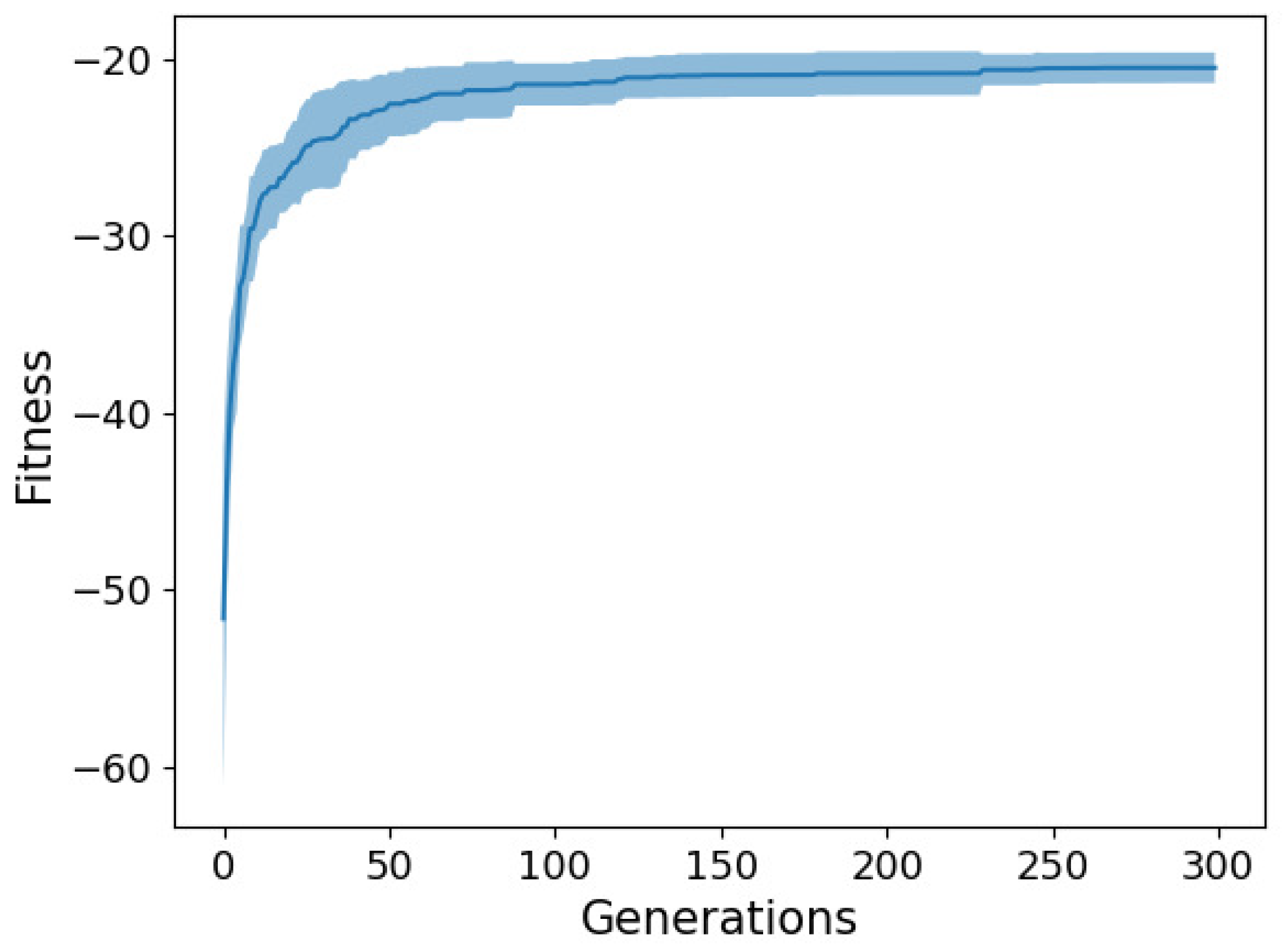
For illustration purposes, Figure 3 and Figure 4 show the fitness trend (i.e., the training RMSE trend), in terms of average (solid line) ± std. dev. (shaded area) across 10 independent runs, for the best solutions found across generations with two selected NEAT configurations on the two datasets, respectively. From the trends, we can conclude that the algorithm quickly converges in about one-third of the budget and then achieves minor improvements in the remaining part of the evolutionary process. Furthermore, we can observe that the method is quite robust across runs, since the std. dev. of the fitness trend is fairly small.

Concerning CMAPSS, the comparative results on the FD001 of all the considered methods are presented in

Table 7. Summary of the comparative analysis based on the test results on CMAPSS (FD001). The symbol “-” indicates not available data. For our SNPS methods, we report the RMSE in terms of mean ± std. dev. across 10 independent runs. For the remaining methods, we report the results from the original papers (std. dev. not provided). The boldface indicates the best value per column.

Methods	Test RMSE	s-Score × (${10}^3$)	Trainable Parameters	Test Execution Time (ms)
MLP [13]	37.36 ± 0.00	6.45	801	93
CNN [13]	18.45 ± 0.00	1.29	6815	151
LSTM [14]	16.14 ± 0.00	0.34	14,681	968
SVM [38]	29.82 ± 0.00	-	-	-
SNPS (1)	29.27 ± 3.76	3.28	263	25
SNPS (2)	31.55 ± 3.61	8.83	365	27
SNPS (3)	29.28 ± 2.99	4.36	60	7
SNPS (4)	20.90 ± 1.52	0.81	334	28
SNPS (5)	20.32 ± 1.54	0.54	232	25
SNPS (6)	20.79 ± 1.58	1.57	285	26

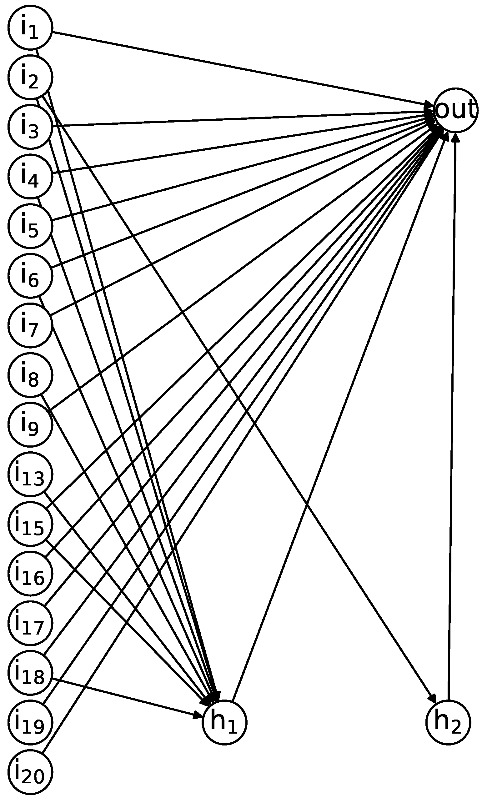
. SNPS (1) to (6) indicate the best SN P systems obtained with each of the six NEAT configurations reported in Table 6. In terms of the test RMSE, all the six results are much better than the MLP, since we can achieve lower RMSE values with a smaller number of trainable parameters. In addition, we observe that the test RMSE of the SVM-based model taken from [38] is placed between the result of the MLP and our best results. Furthermore, the test results of SNPS (4) and (6) are fairly comparable with those obtained by the CNN and the LSTM in terms of test RMSE, but our proposed method achieves these results by using a considerably smaller number of trainable parameters (1–2 orders of magnitude lower). In particular, we should note that the solution that gives the best RMSE, SNPS (5), contains only 232 parameters, while the most complex method in the table, the LSTM, has 14,681 parameters. The architecture of this SNPS is depicted in Figure 5. It should be noted that this system was simplified by removing the nodes and edges that did not have an impact on the output.

Considering the s-score, the values obtained by our proposed method are better than the s-score of the MLP. Compared to the CNN, SNPS (5) gives a better s-score, although its RMSE is slightly worse. This indicates that the proposed method not only speeds up the RUL predictions with comparable accuracy, but also it can be robust to the risk of optimistic RUL predictions.

The importance of reducing the number of parameters can be highlighted by comparing the test execution time. For all the time measurements, we use the same GPU, and the time related to the initialization of the DL library is neglected. Although the test time is not linearly proportional to the number of trainable parameters, there is a positive correlation; our best SNPS in terms of test RMSE that has 232 parameters, i.e., SNPS (5), spends merely 25 ms to compute RUL predictions of the test samples, while a very simple one hidden layer MLP containing 801 parameters takes almost four times as much. Moreover, SNPS (3), which has only 60 parameters, spends only 7 ms to execute the test. In contrast, the CNN and LSTM, which contain a significantly larger number of parameters compared to our models, require a much longer time to complete the test. Thus, the small amount of parameters in our SN P systems represents the main advantage of the proposed method, since it is clear that reducing the number of parameters can reduce the time needed to predict the RUL.

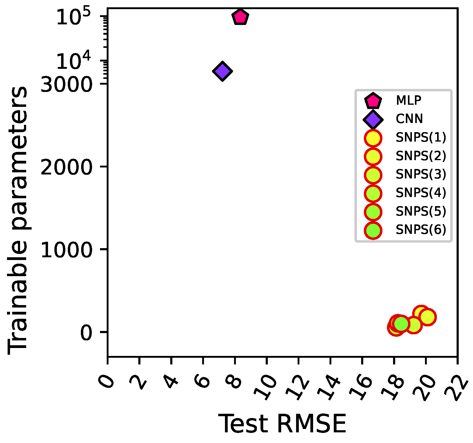
Figure 6 visualizes the trade-offs of the different methods (excluding SVM, for which the number of parameters is not available from [38]) in terms of test RMSE vs. number of parameters. We can observe that the proposed method Pareto dominates the MLP. Among the compared algorithms, the proposed method is clearly the best one in terms of number of trainable parameters. Moreover, compared to the LSTM, the best SNPS architecture we found has an approximately $95\%$ shorter test execution time, with around $95\%$ less parameters, while its test RMSE is only about $15\%$ larger.

Table 8. Summary of the comparative analysis based on the test results on N-CMAPSS (DS02). The symbol “-” indicates not available data. For our SNPS methods, we report the RMSE in terms of mean ± std. dev. across 10 independent runs. For the remaining methods, we report the results from the original papers (std. dev. not provided). The boldface indicates the best value per column.

Methods	Test RMSE	s-Score × (${10}^3$)	Trainable Parameters	Test Execution Time (ms)
MLP [39]	8.34 ± 0.00	20.41	94,701	1223
CNN [39]	7.22 ± 0.00	1.14	5722	1178
SNPS (1)	19.72 ± 0.44	8.39	218	19
SNPS (2)	20.11 ± 0.62	6.53	180	17
SNPS (3)	19.23 ± 0.57	7.92	83	12
SNPS (4)	18.14 ± 0.52	6.39	56	11
SNPS (5)	18.25 ± 0.59	7.69	105	15
SNPS (6)	18.45 ± 0.57	6.48	98	14
$R_{rnd}$	26.85 ± 0.00	276.76	-	-
$R_{\mu }$	18.97 ± 0.00	63.98	-	-

presents the comparative results on the N-CMAPSS dataset of the two deep neural networks taken from [39] and the solutions obtained by our proposed method. It should be noted that compared to the shallow MLP used on the CMAPSS dataset, the number of parameters of the MLP used here is more than two orders of magnitude larger ($\mathrm{94,701}$ vs. 801). On the other hand, the CNN has a comparable number of parameters. We can see that the two deep networks can reach a very low RMSE. However, the CNN shows a better prediction accuracy with a lower number of parameters, although the computation for training this DL architecture is still considerably large [19]. Differently from the results on CMAPSS, the s-score performance of the proposed method is better than that of MLP, but it cannot reach the performance of the CNN. As illustrated in Figure 7, our SN P systems do not outperform the CNN in terms of RMSE, but they have a clear advantage in terms of number of trainable parameters. Especially the best solution in terms of test RMSE, SNPS (4) illustrated in Figure 8, has 56 parameters, and this remarkably simple structure enables predicting RUL very quickly. In fact, the execution time on the test set reported in Table 8 clearly demonstrates this advantage. On this notably larger dataset, the proposed method only takes less than 20 ms to predict the RUL, while the other methods take more than 1 s.

Another advantage of our method relates to memory consumption (which correlates to the number of parameters). Considering that in all the experiments we used the standard 32-bit floating point precision (so that each parameter takes 4 bytes), we can see that the method with the largest number of parameters, the MLP, consumes roughly 370 KB, while our SN P systems take much less than 1 KB. This difference may be crucial for some industrial environments characterized by stringent memory constraints, e.g., due to the use of embedded systems.

Finally, as a further reference, we include in Table 8 two additional RMSE values, namely $R_{rnd}$ and $R_{\mu }$. The test RMSE value of $R_{rnd}$ indicates the performance that may be obtained by randomly choosing an RUL value from the test labels and considering it as an RUL prediction. Therefore, the random performance can be calculated by the RMSE between the test labels and the randomly chosen values. In the case of $R_{\mu }$, we take instead all the RUL values from the test labels and compute their mean. Then, the mean performance is computed by the RMSE between the test labels and their mean. We can see that our results are better than the result of $R_{rnd}$, but only three NEAT configurations perform slightly better than $R_{\mu }$. One additional note is that the test RMSE values of the BPNNs reported in Table 8 are different from those reported in [39], which are based on an early version of DS02 that has a lower noise level on the sensor readings and a sampling rate of $0.1$ Hz.

6. Conclusions

Spiking Neural P (in short, SN P) systems are a bio-inspired computing tool that incorporates the idea of spiking neurons into membrane systems called P systems. These systems have been used for a variety of applications, but so far, they have been handcrafted by human experts for each application. In this paper, we employed a custom neuro-evolutionary algorithm, based on NEAT, to automatically design SN P systems for a given task, with little or no domain knowledge. The proposed method was applied to an RUL prediction task for predictive maintenance, where so far, traditional neural networks have been mainly used. Then, we compared our method to methods from the literature, e.g., based on MLPs and CNNs. The comparative evaluation was based not only on the CMAPSS dataset, which is the de facto standard benchmark in the area of RUL prediction, but also on the N-CMAPSS dataset, which is one of the most up-to-date benchmarks in this area. In the experiments on CMAPSS, we observed that our approach was able to produce SN P systems that are competitive in terms of prediction error but with a much smaller number of trainable parameters. Moreover, in the experiments on the N-CMAPSS dataset, although our approach was not able to outperform the deep neural networks when considering the RMSE, it produced once again much smaller structures (in terms of number of parameters). Overall, our approach provides a reasonable trade-off between performance and number of trainable parameters, so that the proposed SN P systems with optimized structure and parameters can be used as an efficient RUL prediction tool in industrial applications that require finding a compromise between the prediction accuracy and the number of parameters, which in turns correlates with memory consumption (which is a crucial aspect e.g., in embedded systems) and computing time.

References

1. Song, T.; Pan, L.; Wu, T.; Zheng, P.; Wong, M.L.D.; Rodriguez-Paton, A. Spiking Neural P Systems With Learning Functions. IEEE Trans. NanoBiosci. 2019, 18, 176–190. [Google Scholar] [CrossRef] [PubMed]
2. Paun, G. Computing with Membranes. J. Comput. Syst. Sci. 2000, 61, 108–143. [Google Scholar] [CrossRef] [Green Version]
3. Ionescu, M.; Păun, G.; Yokomori, T. Spiking neural P systems. Fundam. Inform. 2006, 71, 279–308. [Google Scholar]
4. Păun, G.; Pérez-Jiménez, M.J.; Rozenberg, G. Spike trains in spiking neural P systems. Int. J. Found. Comput. Sci. 2006, 17, 975–1002. [Google Scholar] [CrossRef] [Green Version]
5. Martín-Vide, C.; Pazos, J.; Păun, G.; Rodríguez-Patón, A. A New Class of Symbolic Abstract Neural Nets: Tissue P Systems. In International Computing and Combinatorics Conference (COCOON); Ibarra, O.H., Zhang, L., Eds.; Springer: Berlin/Heidelberg, Germany, 2002; pp. 290–299. [Google Scholar]
6. Pan, L.; Zeng, X. A note on small universal spiking neural P systems. In Proceedings of the International Workshop on Membrane Computing (WMC), Curtea de Arges, Romania, 24–27 August 2009; Springer: Berlin/Heidelberg, Germany, 2009; pp. 436–447. [Google Scholar]
7. Wang, J.; Hoogeboom, H.J.; Pan, L.; Păun, G.; Pérez-Jiménez, M.J. Spiking neural P systems with weights. Neural Comput. 2010, 22, 2615–2646. [Google Scholar] [CrossRef] [PubMed]
8. Wang, X.; Song, T.; Gong, F.; Zheng, P. On the computational power of spiking neural P systems with self-organization. Sci. Rep. 2016, 6, 27624. [Google Scholar] [CrossRef]
9. Dong, J.; Stachowicz, M.; Zhang, G.; Cavaliere, M.; Rong, H.; Paul, P. Automatic Design of Spiking Neural P Systems Based on Genetic Algorithms. Int. J. Unconv. Comput. 2021, 16, 201–216. [Google Scholar]
10. Casauay, L.J.P.; Cabarle, F.G.C.; Macababayao, I.C.H.; Adorna, H.N.; Zeng, X.; Martínez-Del-Amor, M.Á.; Cruz, R.T.D.L. A Framework for Evolving Spiking Neural P Systems. Int. J. Unconv. Comput. 2021, 16, 271–298. [Google Scholar]
11. Custode, L.L.; Mo, H.; Iacca, G. Neuroevolution of Spiking Neural P Systems. In Applications of Evolutionary Computation; 2022; to appear. [Google Scholar]
12. Stanley, K.O.; Miikkulainen, R. Evolving neural networks through augmenting topologies. Evol. Comput. 2002, 10, 99–127. [Google Scholar] [CrossRef]
13. Sateesh Babu, G.; Zhao, P.; Li, X.L. Deep Convolutional Neural Network Based Regression Approach for Estimation of Remaining Useful Life. In Database Systems for Advanced Applications; Lecture Notes in Computer Science; Navathe, S.B., Wu, W., Shekhar, S., Du, X., Wang, X.S., Xiong, H., Eds.; Springer: Berlin/Heidelberg, Germany, 2016; Volume 9642, pp. 214–228. [Google Scholar] [CrossRef]
14. Zheng, S.; Ristovski, K.; Farahat, A.; Gupta, C. Long Short-Term Memory Network for Remaining Useful Life estimation. In Proceedings of the 2017 IEEE International Conference on Prognostics and Health Management (ICPHM), Dallas, TX, USA, 19–21 June 2017; pp. 88–95. [Google Scholar]
15. Chen, Z.; Wu, M.; Zhao, R.; Guretno, F.; Yan, R.; Li, X. Machine Remaining Useful Life Prediction via an Attention-Based Deep Learning Approach. IEEE Trans. Ind. Electron. 2021, 68, 2521–2531. [Google Scholar] [CrossRef]
16. Mo, H.; Custode, L.L.; Iacca, G. Evolutionary neural architecture search for remaining useful life prediction. Appl. Soft Comput. 2021, 108, 107474. [Google Scholar] [CrossRef]
17. Mo, H.; Lucca, F.; Malacarne, J.; Iacca, G. Multi-Head CNN-LSTM with Prediction Error Analysis for Remaining Useful Life Prediction. In Proceedings of the 2020 27th Conference of Open Innovations Association (FRUCT), Trento, Italy, 7–9 September 2020; pp. 164–171. [Google Scholar]
18. Ye, Z.; Yu, J. Health condition monitoring of machines based on long short-term memory convolutional autoencoder. Appl. Soft Comput. 2021, 107, 107379. [Google Scholar] [CrossRef]
19. Mo, H.; Iacca, G. Multi-Objective Optimization of Extreme Learning Machine for Remaining Useful Life Prediction. In Applications of Evolutionary Computation; 2022; to appear. [Google Scholar]
20. Ma, T.; Hao, S.; Wang, X.; Alfonso Rodriguez-Paton, A.; Wang, S.; Song, T. Double Layers Self-Organized Spiking Neural P Systems With Anti-Spikes for Fingerprint Recognition. IEEE Access 2019, 7, 177562–177570. [Google Scholar] [CrossRef]
21. Peng, H.; Wang, J.; Pérez-Jiménez, M.J.; Wang, H.; Shao, J.; Wang, T. Fuzzy reasoning spiking neural P system for fault diagnosis. Inf. Sci. 2013, 235, 106–116. [Google Scholar] [CrossRef]
22. Wang, T.; Zhang, G.; Zhao, J.; He, Z.; Wang, J.; Perez-Jimenez, M.J. Fault Diagnosis of Electric Power Systems Based on Fuzzy Reasoning Spiking Neural P Systems. IEEE Trans. Power Syst. 2015, 30, 1182–1194. [Google Scholar] [CrossRef]
23. Chen, H.; Ishdorj, T.-O.; Paun, G.; Pérez Jiménez, M.d.J. Spiking neural P systems with extended rules. In Proceedings of the 4th Brainstorming Week on Membrane Computing (BWMC), Sevilla, Spain, 30 January–3 February 2006; Fénix Editora: ETS de Ingeniería Informática. Volume I, pp. 241–265. [Google Scholar]
24. Ishdorj, T.-O.; Leporati, A. Uniform solutions to SAT and 3-SAT by spiking neural P systems with pre-computed resources. Nat. Comput. 2008, 7, 519–534. [Google Scholar] [CrossRef]
25. Leporati, A.; Gutiérrez-Naranjo, M.A. Solving Subset Sum by spiking neural P systems with pre-computed resources. Fundam. Inform. 2008, 87, 61–77. [Google Scholar]
26. Zhang, G.; Rong, H.; Neri, F.; Pérez-Jiménez, M.J. An optimization spiking neural P system for approximately solving combinatorial optimization problems. Int. J. Neural Syst. 2014, 24, 1440006. [Google Scholar] [CrossRef]
27. Qi, F.; Liu, M. Optimization spiking neural P system for solving TSP. In Proceedings of the International Conference on Machine Learning and Intelligent Communications (MLICOM), Shenzhen, China, 26–27 September 2017; Springer: Berlin/Heidelberg, Germany, 2017; pp. 668–676. [Google Scholar]
28. Ionescu, M.; Sburlan, D. Some applications of spiking neural P systems. Comput. Inform. 2008, 27, 515–528. [Google Scholar]
29. Hamabe, R.; Fujiwara, A. Asynchronous SN P systems for logical and arithmetic operations. In Proceedings of the International Conference on Foundations of Computer Science (FCS), Las Vegas, NV, USA, 16–19 July 2012; The Steering Committee of the World Congress in Computer Science. p. 1. [Google Scholar]
30. Song, T.; Zheng, P.; Wong, M.D.; Wang, X. Design of logic gates using spiking neural P systems with homogeneous neurons and astrocytes-like control. Inf. Sci. 2016, 372, 380–391. [Google Scholar] [CrossRef]
31. Peng, X.W.; Fan, X.P.; Liu, J.X. Performing balanced ternary logic and arithmetic operations with spiking neural P systems with anti-spikes. Adv. Mater. Res. 2012, 505, 378–385. [Google Scholar] [CrossRef]
32. Tu, M.; Wang, J.; Peng, H.; Shi, P. Application of Adaptive Fuzzy Spiking Neural P Systems in Fault Diagnosis of Power Systems. Chin. J. Electron. 2014, 23, 87–92. [Google Scholar]
33. Díaz-Pernil, D.; Peña-Cantillana, F.; Gutiérrez-Naranjo, M.A. A parallel algorithm for skeletonizing images by using spiking neural P systems. Neurocomputing 2013, 115, 81–91. [Google Scholar] [CrossRef]
34. Song, T.; Pang, S.; Hao, S.; Rodríguez-Patón, A.; Zheng, P. A parallel image skeletonizing method using spiking neural P systems with weights. Neural Process. Lett. 2019, 50, 1485–1502. [Google Scholar] [CrossRef]
35. Schäfer, P.; Högqvist, M. SFA: A symbolic Fourier approximation and index for similarity search in high dimensional datasets. In Proceedings of the 15th International Conference on Extending Database Technology—EDBT’12, Berlin, Germany, 27–30 March 2012; ACM Press: New York, NY, USA, 2012; p. 516. [Google Scholar]
36. Saxena, A.; Goebel, K.; Simon, D.; Eklund, N. Damage propagation modeling for aircraft engine run-to-failure simulation. In Proceedings of the 2008 International Conference on Prognostics and Health Management, Denver, CO, USA, 6–9 October 2008; IEEE: Piscataway, NJ, USA, 2008; pp. 1–9. [Google Scholar]
37. Arias Chao, M.; Kulkarni, C.; Goebel, K.; Fink, O. Aircraft Engine Run-to-Failure Dataset under Real Flight Conditions for Prognostics and Diagnostics. Data 2021, 6, 5. [Google Scholar] [CrossRef]
38. Louen, C.; Ding, S.X.; Kandler, C. A new framework for remaining useful life estimation using Support Vector Machine classifier. In Proceedings of the 2013 Conference on Control and Fault-Tolerant Systems (SysTol), Nice, France, 9–11 October 2013; IEEE: Piscataway, NJ, USA, 2013; pp. 228–233. [Google Scholar]
39. Arias Chao, M.; Kulkarni, C.; Goebel, K.; Fink, O. Fusing physics-based and deep learning models for prognostics. Reliab. Eng. Syst. Saf. 2022, 217, 107961. [Google Scholar] [CrossRef]
40. McIntyre, A.; Kallada, M.; Miguel, C.G.; da Silva, C.F. Neat-Python. Available online: https://github.com/CodeReclaimers/neat-python (accessed on 10 November 2021).
Figure 1. Flow chart of a data-driven RUL prediction task.
Algorithms 15 00098 g001
Figure 2. Illustration of the Symbolic Fourier Approximation process. X i denotes a selected Fourier coefficient, and o i represents each output symbol from the SFA.
Algorithms 15 00098 g002
Figure 3. Fitness across generations (mean ± std. dev. across 10 independent runs) for SNPS (5) on CMAPSS (FD001).
Algorithms 15 00098 g003
Figure 4. Fitness across generations (mean ± std. dev. across 10 independent runs) for SNPS (4) on N-CMAPSS (DS02).
Algorithms 15 00098 g004
Figure 5. Best SN P system evolved for the RUL prediction task on CMAPSS (FD001).
Algorithms 15 00098 g005
Figure 6. Trade-off between test RMSE and number of trainable parameters for the methods considered in the experimentation on CMAPSS (FD001).
Algorithms 15 00098 g006
Figure 7. Trade-off between test RMSE and number of trainable parameters for the methods considered in the experimentation on N-CMAPSS (DS02).
Algorithms 15 00098 g007
Figure 8. Best SN P system evolved for the RUL prediction task on N-CMAPSS (DS02).
Algorithms 15 00098 g008