A Variable Step Size Normalized Least-Mean-Square Algorithm Based on Data Reuse

Abstract

The principal issue in acoustic echo cancellation (AEC) is to estimate the impulse response between the loudspeaker and microphone of a hands-free communication device. This application can be addressed as a system identification problem, which can be solved by using an adaptive filter. The most common one for AEC is the normalized least-mean-square (NLMS) algorithm. It is known that the overall performance of this algorithm is controlled by the value of its normalized step size parameter. In order to obtain a proper compromise between the main performance criteria (e.g., convergence rate/tracking versus accuracy/robustness), this specific term of the NLMS algorithm can be further controlled and designed as a variable parameter. This represents the main motivation behind the development of variable step size algorithms. In this paper, we propose a variable step size NLMS (VSS-NLMS) algorithm that exploits the data reuse mechanism, which aims to improve the convergence rate/tracking of the algorithm by reusing the same set of data (i.e., the input and reference signals) several times. Nevertheless, we involved an equivalent version of the data reuse NLMS, which provides the convergence modes of the algorithm. Based on this approach, a sequence of normalized step sizes can be a priori scheduled, which is advantageous in terms of the computational complexity. The simulation results in the context of AEC supported the good performance features of the proposed VSS-NLMS algorithm.

1. Introduction

The normalized least-mean-square (NLMS) algorithm is the workhorse in many practical applications of adaptive filtering [1,2,3]. The main reasons behind its popularity consist of its simple and efficient implementation, together with fairly reasonable performance, in terms of the convergence rate, tracking, and accuracy of the solution. Nevertheless, there is always a need to improve the performance features of the NLMS algorithm, especially in challenging scenarios, e.g., when using highly correlated input signals and/or dealing with long-length adaptive filters. In this framework, a very important application is acoustic echo cancellation (AEC) [4,5,6], where the input signal is mainly speech (i.e., a nonstationary and highly correlated sequence), while the impulse response of the acoustic echo path is usually of the order of hundreds or even thousands of coefficients.

There are several strategies to improve the performance of the NLMS algorithm in AEC scenarios. Among them, proportionate NLMS algorithms exploit the sparseness nature of the echo paths to increase the convergence rate and tracking of the adaptive filter [7,8,9,10,11,12,13]. Besides, variable step size NLMS (VSS-NLMS) algorithms are designed to achieve a proper compromise between the convergence rate and misadjustment (i.e., accuracy of the estimate) [14,15,16,17,18]. Moreover, the data reuse approach consists of performing more than one filter update for the same set of data (i.e., the input and reference signals), thus targeting a higher convergence rate [19,20,21,22,23,24,25].

In this short communication, we focused on the data reuse NLMS algorithm from a different perspective, showing how it can be exploited in order to develop an improved NLMS version with variable step sizes. As compared to other previous works related to the data reuse approach, the proposed VSS-NLMS algorithm uses a sequence of scheduled step size parameters. These values are a priori computed by exploiting the convergence modes of the data reuse NLMS algorithm. On the contrary, in [24], the variable step size (VSS) from [14] was used in conjunction with the data reuse NLMS algorithm from [21], thus resulting in a new version that was similar to an affine projection algorithm with VSS parameter. Furthermore, in [25], the data reuse approach was applied to an optimized least-mean-square algorithm, which behaves similar to a VSS version. In these previous works, the VSS parameter was evaluated within each iteration of the algorithm, which is fundamentally different as compared to the current proposed approach, where the step size parameters were a priori computed and scheduled within the algorithm.

Our main application framework was AEC [4], where the main goal was to estimate the impulse response between the loudspeaker and microphone of a hands-free communication device. Basically, we dealt with a system identification problem, which can be solved by using an adaptive filter. Currently, hands-free communication devices are involved in many popular applications, such as mobile telephony and teleconferencing systems. Due to their specific features, they can be used in a wide range of environments with different acoustic characteristics. In this context, an important issue that has to be addressed when dealing with such devices is the acoustic coupling between the loudspeaker and microphone. In other words, besides the voice of the near-end speaker and the background noise, the microphone of the hands-free equipment captures another signal (coming from its own loudspeaker), known as the acoustic echo. Depending on the environments’ characteristics, this phenomenon can be very disturbing for the far-end speaker, which hears a replica of her/his own voice. From this point of view, there is a need to enhance the quality of the microphone signal by canceling the unwanted acoustic echo. The most reliable solution to this problem is the use of an adaptive filter that generates at its output a replica of the echo, which is further subtracted from the microphone signal [4,5,6]. Consequently, the adaptive filter has to model an unknown system, i.e., the acoustic echo path between the loudspeaker and microphone.

Even if the problem formulation is straightforward, the specific features of AEC represent a challenge for any adaptive algorithm. First, the acoustic echo paths have excessive lengths in time (up to hundreds of milliseconds), due to the slow speed of sound in the air, together with multiple reflections caused by the environment; therefore, long-length adaptive filters are required (hundreds or even thousands of coefficients), influencing the convergence rate of the algorithm. Second, the acoustic echo paths are time-variant systems (depending on the temperature, pressure, humidity, and movement of objects or bodies), requiring good tracking capabilities for the echo canceler. Third, the input of the adaptive filter (i.e., the far-end signal) is mainly speech, which is a nonstationary and highly correlated signal that can influence the overall performance of the adaptive algorithm.

Since the conventional NLMS algorithm uses a constant step size parameter to control its performances, a compromise should be made when choosing this value. It is known that a large value implies a fast convergence rate and tracking, while a small value leads to low misadjustment and good robustness features. Since in AEC, there is a need for all these performance criteria, the step size should be controlled; therefore, a VSS version represents a more reliable choice. In addition, for real-world AEC applications, it is highly desirable to use nonparametric algorithms, in the sense that no information about the acoustic environment is required. Nevertheless, we should note that the applications of the VSS-NLMS algorithms are not limited only to the framework of AEC. Different other application areas can be explored in the field of communication systems, such as the carrier phase recovery, e.g., see [26,27] and the references therein.

Following this Introduction, in Section 2, we present the data reuse NLMS algorithm, but using a computationally efficient method to exploit the data reuse process, thus keeping almost the same complexity as the conventional version. Then, in Section 3, we develop a VSS-NLMS algorithm based on the data reuse approach. Simulation results in the context of AEC are provided in Section 4 in order to support the performance of the proposed VSS-NLMS algorithm. Finally, several conclusions are summarized in Section 5. The acronyms used in this paper are provided in

Table A1. List of acronyms.

Acronym	Definition
AEC	acoustic echo cancellation
AR	autoregressive
AR(1)	first-order autoregressive process
ENR	echo-to-noise ratio
NLMS	normalized least-mean-square
NPVSS-NLMS	nonparametric variable step size normalized least-mean-square
VSS	variable step size
VSS-NLMS	variable step size normalized least-mean-square

in Appendix A, while the notation and symbols are summarized in

Table A2. Notation, symbols, and parameters.

Notation	Definition
${}^T$	transpose of a vector or a matrix
$∥·∥$	${\ell }_2$ (Euclidean) norm
$E\left[·\right]$	mathematical expectation
$\log (·)$	natural logarithm
${\log }_{10}(·)$	decimal logarithm
$\lceil ·\rceil$	ceiling function
n	discrete-time index
L	length of the filter
$\lambda =1-1/\left(KL\right)$	weighting parameter, with $K\ge 1$
$\gamma =1-1/\left(QL\right)$	weighting parameter, with $Q=3K$
$\xi$	specific threshold, with $\xi =1.5$
$\alpha$	normalized step size parameter of the NLMS algorithm
	(lower bound of the VSS-NLMS algorithm)
$\mu \left(n\right)$	variable step size parameter of the VSS-NLMS algorithm
$\tilde{\mu }\left(n\right)$	variable step size parameter of the NPVSS-NLMS algorithm
$\mathbf{h}$	impulse response of the unknown system (echo path)
$\widehat{\mathbf{h}}\left(n\right)$	impulse response of the adaptive filter
${\widehat{\mathbf{h}}}_k\left(n\right)$	impulse response of the adaptive filter in the kth data reuse iteration
$k_{\max }$	maximum number of data reuse iterations
${\alpha }_{\max }$	maximum value of the normalized step size
q	specific step of the data reuse iteration, with $q=1,2,\dots ,k_{\max }$
l	specific parameter of the VSS-NLMS algorithm, with $0<l\le 1$
$x\left(n\right)$	input signal (far-end signal)
$\mathbf{x}\left(n\right)$	vector containing the most recent L time samples of the input signal
$d\left(n\right)$	reference or desired signal (microphone signal)
$y\left(n\right)$	output signal of the unknown system (echo signal)
$e\left(n\right)$	a priori error signal
$e_1\left(n\right)$	a posteriori error signal
$e_k\left(n\right)$	kth-order a posteriori error signal
$v\left(n\right)$	additive noise signal (background noise)
${\sigma }_v^2$	variance of the noise signal
${\sigma }_y^2$	variance of the output (echo) signal
${\widehat{\sigma }}_e^2\left(n\right)$	power estimate of the error signal
${\widehat{\sigma }}_v^2\left(n\right)$	power estimate of the noise signal

from the same section.

2. Data Reuse NLMS Algorithm

The conventional NLMS algorithm [1,3] is defined by two main equations, which provide the error signal and the filter update, respectively, as follows:

$$\begin{array}{cc}\hfill e\left(n\right)& =d\left(n\right)-{\mathbf{x}}^T\left(n\right)\widehat{\mathbf{h}}(n-1),\hfill \end{array}$$

(1)

$$\begin{array}{cc}\hfill \widehat{\mathbf{h}}\left(n\right)& =\widehat{\mathbf{h}}(n-1)+\frac{\alpha \mathbf{x}\left(n\right)e\left(n\right)}{{\mathbf{x}}^T\left(n\right)\mathbf{x}\left(n\right)},\hfill \end{array}$$

(2)

where $e\left(n\right)$ is the a priori error signal at the discrete-time index n, $d\left(n\right)$ is the desired (or reference) signal, $\mathbf{x}\left(n\right)={\left[\begin{array}{cccc}x\left(n\right)& x(n-1)& \cdots & x(n-L+1)\end{array}\right]}^T$ is a vector containing the most recent L time samples of the zero-mean input signal $x\left(n\right)$, the superscript ${}^T$ denotes the transpose operator, $\widehat{\mathbf{h}}\left(n\right)={\left[\begin{array}{cccc}{\widehat{h}}_0\left(n\right)& {\widehat{h}}_1\left(n\right)& \cdots & {\widehat{h}}_{L-1}\left(n\right)\end{array}\right]}^T$ is the adaptive filter (of length L) at the discrete-time index n, which is an estimate of the unknown impulse response, and $\alpha$ is the normalized step size parameter of the NLMS algorithm. Theoretically, the range for this parameter is $0<\alpha <2$, but practically, the recommended choice is $0<\alpha \le 1$ [2]. For the sake of simplicity, we omitted in the developments the regularization parameter $\delta >0$ [28], which is usually added to the denominator in (2).

Based on the adaptive filter coefficients at the discrete-time index n, we may also define the a posteriori error signal as:

$$\begin{array}{cc}\hfill e_1\left(n\right)& =d\left(n\right)-{\mathbf{x}}^T\left(n\right)\widehat{\mathbf{h}}\left(n\right).\hfill \end{array}$$

(3)

Using (1) and (2) in (3), we can further develop the previous expression of the a posteriori error, which results in:

$$\begin{array}{cc}\hfill e_1\left(n\right)& =\left(1-\alpha \right)e\left(n\right).\hfill \end{array}$$

(4)

It can be noticed that the a posteriori error is canceled for $\alpha =1$ (assuming that $e\left(n\right)\ne 0$).

Now, let us consider that we perform multiple iterations for the NLMS algorithm using the same input data $\mathbf{x}\left(n\right)$ and reference signal $d\left(n\right)$, i.e., performing the data reuse process [19,20,21,22,23,24,25]. Hence, in the first step (using (1), (2), and (4)), we have:

$$\begin{array}{cc}\hfill {\widehat{\mathbf{h}}}_1\left(n\right)& =\widehat{\mathbf{h}}\left(n\right)+\frac{\alpha \mathbf{x}\left(n\right)e_1\left(n\right)}{{\mathbf{x}}^T\left(n\right)\mathbf{x}\left(n\right)}\hfill \\ \hfill & =\widehat{\mathbf{h}}(n-1)+\frac{[1-{(1-\alpha )}^2]\mathbf{x}\left(n\right)e\left(n\right)}{{\mathbf{x}}^T\left(n\right)\mathbf{x}\left(n\right)}.\hfill \end{array}$$

(5)

Then, by repeating the process, we obtain:

$$\begin{array}{cc}\hfill e_2\left(n\right)& =d\left(n\right)-{\mathbf{x}}^T\left(n\right){\widehat{\mathbf{h}}}_1\left(n\right)\hfill \\ & ={\left(1-\alpha \right)}^{2}e\left(n\right),\hfill \end{array}$$

(6)

$$\begin{array}{cc}\hfill {\widehat{\mathbf{h}}}_2\left(n\right)& ={\widehat{\mathbf{h}}}_1\left(n\right)+\frac{\alpha \mathbf{x}\left(n\right)e_2\left(n\right)}{{\mathbf{x}}^T\left(n\right)\mathbf{x}\left(n\right)}\hfill \\ & =\widehat{\mathbf{h}}(n-1)+\frac{[1-{(1-\alpha )}^3]\mathbf{x}\left(n\right)e\left(n\right)}{{\mathbf{x}}^T\left(n\right)\mathbf{x}\left(n\right)},\hfill \end{array}$$

(7)

and so on.

Using mathematical induction, it results that the kth-order a posteriori error is:

$$\begin{array}{c}\hfill e_k\left(n\right)={\left(1-\alpha \right)}^{k}e\left(n\right)\end{array}$$

(8)

and the kth-order update is given by:

$$\begin{array}{c}\hfill {\widehat{\mathbf{h}}}_k\left(n\right)=\widehat{\mathbf{h}}(n-1)+\frac{[1-{(1-\alpha )}^{k+1}]\mathbf{x}\left(n\right)e\left(n\right)}{{\mathbf{x}}^T\left(n\right)\mathbf{x}\left(n\right)},\end{array}$$

(9)

which is similar to the original update (2), but using the normalized step size:

$$\begin{array}{c}\hfill {\alpha }_k=1-{(1-\alpha )}^{k+1}.\end{array}$$

(10)

In other words, performing multiple iterations for the same set of data is equivalent to increasing the value of the normalized step size, thus leading to a faster convergence mode [1,2,3].

A few remarks can be outlined based on the previous results, as follows:

(1) If $\alpha =1$, then $e_k\left(n\right)=0$ and ${\alpha }_k=1$ for any value of k. This supports the well-known fact that the value of the normalized step size $\alpha =1$ provides the fastest convergence mode;

(2) For any $0<\alpha <1$, $e_k{\left(n\right)|}_{k\to \infty }=0$;

(3) For any $0<\alpha <1$, ${\alpha }_k{|}_{k\to \infty }=1$. This is shown in Figure 1, where the parameter ${\alpha }_k$ is plotted for different values of $\alpha$. These curves can be interpreted as the data reuse convergence modes of the NLMS algorithm, for a certain value of $\alpha$.

In addition, based on (10), we can easily evaluate the number of data reuse iterations, $k_{\max }$, required to attain a certain (maximum) value of the normalized step size, ${\alpha }_{\max }$, starting from a given value of $\alpha$. Thus, we can write:

$$\begin{array}{c}\hfill 1-{(1-\alpha )}^{k_{\max }+1}={\alpha }_{\max },\end{array}$$

(11)

which results in:

$$\begin{array}{c}\hfill k_{\max }=⌈\frac{\log (1-{\alpha }_{\max })}{\log (1-\alpha )}⌉-1,\end{array}$$

(12)

where $\lceil ·\rceil$ denotes the ceiling function and $\log (·)$ stands for the natural logarithm.

3. Variable Step Size NLMS Algorithm

Based on the previous considerations, we can design a simple VSS-NLMS algorithm, by implementing the previous approach in a “reverse” manner, using scheduled normalized step sizes. Thus, given the lower and the upper bounds for the normalized step size parameter, i.e., $\alpha$ and ${\alpha }_{\max }$, respectively, the update equation that defines the proposed VSS-NLMS algorithm is:

$$\begin{array}{cc}\hfill \widehat{\mathbf{h}}\left(n\right)& =\widehat{\mathbf{h}}(n-1)+\frac{\mu \left(n\right)\mathbf{x}\left(n\right)e\left(n\right)}{{\mathbf{x}}^T\left(n\right)\mathbf{x}\left(n\right)},\hfill \end{array}$$

(13)

where the variable step size parameter $\mu \left(n\right)$ is evaluated as follows (using (10) and (12)):

• Step 1: $\mu \left(n\right)={\alpha }_{k_{\max }-q+1}$, for $q=1,2,\dots ,k_{\max }$ and $n=(q-1)\lceil lL\rceil +1,\dots ,q\lceil lL\rceil$ (with $0<l\le 1$);
• Step 2: $\mu \left(n\right)=\alpha$, for $n>k_{\max }\lceil lL\rceil$;
• Step 3: if ${\sigma }_e^2\left(n\right)>\xi {\sigma }_v^2$ (with $1<\xi <2$) for $n>k_{\max }\lceil lL\rceil$, then go to Step 1;

where ${\sigma }_e^2\left(n\right)$ denotes the variance of the a priori error signal, ${\sigma }_v^2$ is the power of the system noise (i.e., the external noise that usually corrupts the reference signal), and $k_{\max }$ results based on (12), according to the values of $\alpha$ and ${\alpha }_{\max }$.

In other words, in Step 1, the algorithm uses the normalized step sizes in the following order: ${\alpha }_{k_{\max }}$, ${\alpha }_{k_{\max }-1}$, ${\alpha }_{k_{\max }-2}$, …, ${\alpha }_1$. Each value is used for $\lceil lL\rceil$ iterations, with $0<l\le 1$. For tracking purposes, in order to not stall the algorithm in Step 2 (i.e., when the lower bound of the normalized step size parameter $\alpha$ is used), the condition from Step 3 is introduced. The power estimates required in Step 3 can be recursively evaluated as:

$$\begin{array}{cc}\hfill {\widehat{\sigma }}_e^2\left(n\right)& =\lambda {\widehat{\sigma }}_e^2(n-1)+(1-\lambda )e^2\left(n\right),\hfill \end{array}$$

(14)

$$\begin{array}{cc}\hfill {\widehat{\sigma }}_v^2\left(n\right)& =\gamma {\widehat{\sigma }}_v^2(n-1)+(1-\gamma )e^2\left(n\right),\hfill \end{array}$$

(15)

where $\lambda =1-1/\left(KL\right)$ and $\gamma =1-1/\left(QL\right)$, with $K>1$ and $Q>K$ [29]. The power estimate of the system noise can be roughly estimated from the error signal by using a larger smoothing parameter $\gamma$. By checking the condition from Step 3, we can identify the change of the system (in a system identification scenario) and reset the step size of the algorithm. Of course, more complex/performant detectors can be used in Step 3 [15], but this is beyond the scope of this paper.

The main parameters to be set are $k_{\max }$ and l. The first parameter, $k_{\max }$, is related to the maximum value of the normalized step size, ${\alpha }_{\max }$, as shown in (12). For example, if we consider ${\alpha }_{\max }=0.99$ (which is high enough and very close to the fastest convergence mode) and the lower bound $\alpha \ll 1$ (so that $\log (1-\alpha )\approx -\alpha$), according to (12) we obtain:

$$\begin{array}{c}\hfill k_{\max }\approx ⌈\frac{\log \left(0.01\right)}{-\alpha }⌉-1\approx ⌈\frac{5}{\alpha }⌉.\end{array}$$

(16)

The second parameter, l (with $0<l\le 1$), determines how many iterations (i.e., $\lceil lL\rceil$) the algorithm will use a certain value of the step size (see Step 1). As we can notice from Step 2, the algorithm will reach the lower bound of the normalized step size $\alpha$ after $k_{\max }\lceil lL\rceil$ iterations; from this point of view, it is not recommended to set a very low value of $\alpha$ (e.g., $\alpha <0.01$), which leads to a high value of $k_{\max }$, according to (16). Since the convergence rate of the NLMS-based algorithms depends on the character of the input signal [1,2,3] (in terms of the condition number of the correlation matrix), the value of l should be chosen accordingly. For example, for white Gaussian inputs, we can choose a smaller value of l, e.g., $l<0.3$. For more correlated inputs (such as autoregressive processes), the value of l should be increased, e.g., $0.3\le l<0.5$. Furthermore, for more challenging signals such as speech (i.e., highly correlated and nonstationary), the value of l could be even higher, e.g., $0.5\le l\le 1$.

The computational complexity of the proposed VSS-NLMS algorithm is similar to the complexity of the conventional NLMS benchmark, since the values of the step size parameters of the VSS-NLMS algorithm are a priori computed and scheduled based on (10) and (12); thus, these values can be used directly in Steps 1 and 2 of the algorithm, as describe before. The only extra computational amount is required in Step 3 of the VSS-NLMS algorithm, which is mainly related to the power estimates from (14) and (15). Nevertheless, this step requires only 5 multiplications, 2 additions, and 1 comparison, which represents a negligible computational effort as compared to the overall complexity of the conventional NLMS algorithm that is proportional to $\mathcal{O}\left(L\right)$, especially for very large values of L as in the context of AEC.

In addition, the proposed VSS-NLMS does not require additional parameters from the environment, so it can be considered a nonparametric algorithm [14]. Of course, it would be very useful to find more practical ways to set (or adjust) the parameter l within the algorithm, based on the convergence status of the adaptive filter, but this will be the subject for future works.

4. Simulation Results

Simulations were performed in the context of AEC, in a single-talk scenario [4,5,6]. In this case, the microphone (reference/desired) signal results in:

$$\begin{array}{cc}\hfill \mathbf{d}\left(n\right)& ={\mathbf{h}}^T\mathbf{x}\left(n\right)+v\left(n\right)\hfill \\ \hfill & =y\left(n\right)+v\left(n\right),\hfill \end{array}$$

(17)

where $\mathbf{h}$ contains the coefficients of the acoustic impulse response (of length L), $\mathbf{x}\left(n\right)$ contains the last L time samples of the far-end signal (i.e., the input signal), $v\left(n\right)$ is the background noise, and $y\left(n\right)={\mathbf{h}}^T\mathbf{x}\left(n\right)$ represents the echo signal. In this framework, the main goal is to identify the acoustic echo path, $\mathbf{h}$, with an adaptive filter, $\widehat{\mathbf{h}}\left(n\right)$.

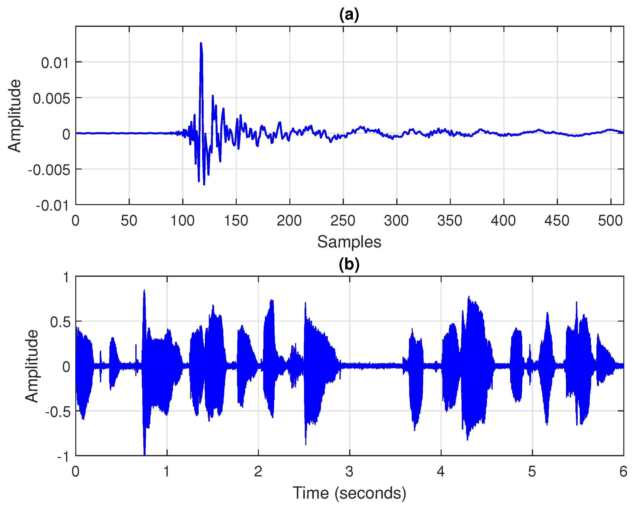
In our experiments, it was considered that $v\left(n\right)$ is a white Gaussian noise, so that the echo-to-noise ratio (ENR) was 20 dB. The ENR is defined as ${\sigma }_y^2/{\sigma }_v^2$, where ${\sigma }_y^2$ denotes the variance of the echo signal. The acoustic echo path $\mathbf{h}$ was obtained from a measured acoustic impulse response using $L=512$ coefficients (depicted in Figure 2a and available at www.comm.pub.ro/plant, accessed on 24 February 2022), and the same length was used for the adaptive filter, using a sampling rate of 8 kHz. Three types of input signals were considered: (i) a white Gaussian noise, (ii) a first-order autoregressive process, referred to as AR(1), which was obtained by filtering a white Gaussian noise through a first-order autoregressive model with a pole at $0.8$, and (iii) a recorded speech sequence (depicted in Figure 2b); for a longer simulation time (as needed in some experiments), this voice signal can be simply repeated several times. The experimental framework is summarized in

Table A3. Experimental framework.

Filter Length	Echo-to-Noise Ratio	Input Signal
$L=512$	$\mathrm{ENR}=20$ dB	white Gaussian noise
		AR(1) process
		speech

in Appendix A. In the middle of some simulations, an echo path change scenario was simulated by shifting the acoustic impulse response to the right by 12 samples, in order to assess the tracking capabilities of the algorithms. The performance measure used in all the experiments was the normalized misalignment (in dB), which is evaluated as:

$$\begin{array}{c}\hfill \mathrm{NM}\left(n\right)=20{\log }_{10}\frac{∥\mathbf{h}-\widehat{\mathbf{h}}\left(n\right)∥}{∥\mathbf{h}∥},\end{array}$$

(18)

where $∥·∥$ denotes the Euclidean norm.

The parameters of the proposed VSS-NLMS algorithm were set as follows. Based on (16), we set $k_{\max }=\lceil 5/\alpha \rceil$, using different values for the lower bound of the normalized step size parameter $\alpha$. The power estimates from (14) and (15) were computed using $K=2$ for the white Gaussian input and $K=6$ for the AR(1) process or speech sequence [14]; also, we used $Q=3K$ and $\xi =1.5$ [29]. The main parameters of the algorithms used in comparisons are provided in

Table A4. Main parameters of the algorithms.

Algorithm	Parameters
NLMS	$\alpha$ (normalized step size)
NPVSS-NLMS	${\sigma }_v^2$ (known or estimated)	K
VSS-NLMS	$\alpha$ (lower bound)	K	l

in Appendix A, while their main values are summarized in

Table A5. Settings of the main parameters.

↓Parameters/$\overrightarrow{\mathrm{Inputs}}$	White Gaussian Noise	AR(1) Process	Speech Sequence
l	$0.1$	$0.3$	$0.5$
K	2	6	6

from the same section.

First, we evaluated the influence of the parameter l on the performance of the proposed algorithm (using the lower bound $\alpha =0.05$), for different types of input signals. The results are given in Figure 3, Figure 4 and Figure 5, using white Gaussian noise, the AR(1) process, and the speech signal, respectively. These results supported the discussion from Section 3, concerning the influence of the parameter l (and the recommended choices). Consequently, in the following simulations, we use $l=0.1$ for white Gaussian inputs, $l=0.3$ for the AR(1) process, and $l=0.5$ for the speech signal.

Next, the performance of the VSS-NLMS algorithm was evaluated for different values of the lower bound of the normalized step size parameter, i.e., $\alpha =0.1,0.05,0.03$, and $0.01$. The results are given in Figure 6, using a white Gaussian noise as the input. It can be noticed that the algorithm was efficient for different values of $\alpha$. However, as was explained in Section 3, it is not recommended to choose a very small value of this lower bound.

In the following experiments, the nonparametric VSS-NLMS (NPVSS-NLMS) algorithm proposed in [14] is introduced for comparison, assuming that the true power of the system noise, ${\sigma }_v^2$, is available for this algorithm. The update of the NPVSS-NLMS algorithm is:

$$\begin{array}{cc}\hfill \widehat{\mathbf{h}}\left(n\right)& =\widehat{\mathbf{h}}(n-1)+\frac{\tilde{\mu }\left(n\right)\mathbf{x}\left(n\right)e\left(n\right)}{{\mathbf{x}}^T\left(n\right)\mathbf{x}\left(n\right)},\hfill \end{array}$$

(19)

where:

$$\begin{array}{cc}\hfill \tilde{\mu }\left(n\right)& =\left\{\begin{array}{cc}1-\frac{{\sigma }_v^2}{{\widehat{\sigma }}_e^2\left(n\right)},\hfill & \mathrm{if}{\widehat{\sigma }}_e^2\left(n\right)\ge {\sigma }_v^2\hfill \\ \hfill & \hfill & \\ 0,\hfill & \mathrm{otherwise}\hfill \end{array}\right.\hfill \end{array}$$

(20)

and ${\widehat{\sigma }}_e^2\left(n\right)$ was evaluated similar to (14). Furthermore, a very small positive constant should be added to the denominator of $\tilde{\mu }\left(n\right)$, in order to avoid any potential division by zero related to the estimation of ${\widehat{\sigma }}_e^2\left(n\right)$. It should be outlined that the NPVSS-NLMS algorithm is usually considered as a benchmark (for many VSS-NLMS algorithms), due to its good performance and practical features. In the following experiments, the proposed VSS-NLMS algorithm uses the lower bound value $\alpha =0.03$. In order to test the tracking capabilities of the algorithms, an echo path change scenario was considered. All three types of input signals were used, i.e., white Gaussian noise, the AR(1) process, and speech; the results are provided in Figure 7, Figure 8 and Figure 9, respectively. It can be noticed that the NPVSS-NLMS algorithm outperformed the proposed VSS-NLMS algorithm in the case of the white Gaussian input. However, the proposed algorithm performed better for the AR(1) process and speech inputs.

Finally, a variation of the ENR was considered, in order to assess the robustness of the algorithms. In Figure 10, the ENR decreased from 20 dB to 10 dB after 120 s. In this experiment, the input signal was speech. Here, we considered that the initial value of ${\sigma }_v^2$ was available for the NPVSS-NLMS algorithm, but not the new one (i.e., after the decrease of the ENR). As expected, the proposed VSS-NLMS algorithm reacted similar to the NLMS algorithm with the smaller normalized step size, outperforming the NPVSS-NLMS algorithm.

5. Conclusions

In this short communication, we developed a simple VSS-NLMS algorithm from a data reuse perspective. The analysis of the data reuse process in conjunction with the NLMS algorithm revealed the convergence modes of this algorithm. As a consequence, a sequence of normalized step sizes can be a priori scheduled to further design a VSS mechanism. Therefore, the resulting VSS-NLMS algorithm based on this approach had almost the same computational complexity as the conventional NLMS algorithm. Simulations were performed in the context of acoustic echo cancellation, and the results indicated the good performance of the proposed algorithm, in terms of its convergence rate, tracking capability, and accuracy of the estimate. In future works, we plan to implement and assess the performance of the proposed VSS-NLMS algorithm in a real-world experimental framework of an AEC application. In addition, we aim to extend the solution toward the affine projection algorithm, targeting further performance improvements, especially in terms of the convergence rate and tracking.

References

1. Haykin, S. Adaptive Filter Theory, 4th ed.; Prentice-Hall: Upper Saddle River, NJ, USA, 2002. [Google Scholar]
2. Benesty, J.; Huang, Y. (Eds.) Adaptive Signal Processing—Applications to Real-World Problems; Springer: Berlin, Germany, 2003. [Google Scholar]
3. Diniz, P.S.R. Adaptive Filtering: Algorithms and Practical Implementation, 4th ed.; Springer: New York, NY, USA, 2013. [Google Scholar]
4. Gay, S.L.; Benesty, J. (Eds.) Acoustic Signal Processing for Telecommunication; Kluwer Academic Publisher: Boston, MA, USA, 2000. [Google Scholar]
5. Benesty, J.; Gänsler, T.; Morgan, D.R.; Sondhi, M.M.; Gay, S.L. Advances in Network and Acoustic Echo Cancellation; Springer: Berlin, Germany, 2001. [Google Scholar]
6. Hänsler, E.; Schmidt, G. Acoustic Echo and Noise Control—A Practical Approach; Wiley: Hoboken, NJ, USA, 2004. [Google Scholar]
7. Duttweiler, D.L. Proportionate normalized least-mean-squares adaptation in echo cancelers. IEEE Trans. Speech Audio Process. 2000, 8, 508–518. [Google Scholar] [CrossRef] [Green Version]
8. Benesty, J.; Gay, S.L. An improved PNLMS algorithm. In Proceedings of the 2002 IEEE International Conference on Acoustics, Speech, and Signal Processing, Orlando, FL, USA, 13–17 May 2002. [Google Scholar]
9. Deng, H.; Doroslovački, M. Proportionate adaptive algorithms for network echo cancellation. IEEE Trans. Signal Process. 2006, 54, 1794–1803. [Google Scholar] [CrossRef]
10. Loganathan, P.; Khong, A.W.; Naylor, P. A class of sparseness-controlled algorithms for echo cancellation. IEEE Trans. Audio Speech Lang. Process. 2009, 17, 1591–1601. [Google Scholar] [CrossRef]
11. Yang, Z.; Zheng, Y.R.; Grant, S.L. Proportionate affine projection sign algorithms for network echo cancellation. IEEE Trans. Audio Speech Lang. Process. 2011, 19, 2273–2284. [Google Scholar] [CrossRef]
12. Liu, J.; Grant, S.L. Proportionate adaptive filtering for block-sparse system identification. IEEE/ACM Trans. Audio Speech Lang. Process. 2016, 24, 623–630. [Google Scholar] [CrossRef] [Green Version]
13. Radhika, S.; Albu, F.; Chandrasekar, A. Proportionate maximum versoria criterion based adaptive algorithm for sparse system identification. IEEE Trans. Circuits Syst. II Express Briefs 2021, 69, 1902–1906. [Google Scholar] [CrossRef]
14. Benesty, J.; Rey, H.; Vega, L.R.; Tressens, S. A nonparametric VSS NLMS algorithm. IEEE Signal Process. Lett. 2006, 13, 581–584. [Google Scholar] [CrossRef]
15. Iqbal, M.A.; Grant, S.L. Novel variable step size NLMS algorithms for echo cancellation. In Proceedings of the 2008 IEEE International Conference on Acoustics, Speech and Signal Processing, Las Vegas, NV, USA, 31 March–4 April 2008; pp. 241–244. [Google Scholar]
16. Rotaru, M.; Albu, F.; Coandă, H. A variable step size modified decorrelated NLMS algorithm for adaptive feedback cancellation in hearing aids. In Proceedings of the 2012 10th International Symposium on Electronics and Telecommunications, Timisoara, Romania, 15–16 November 2012. [Google Scholar]
17. Zhang, S.; Zhang, J.; Han, H. Robust variable step size decorrelation normalized least-mean-square algorithm and its application to acoustic echo cancellation. IEEE/ACM Trans. Audio Speech Lang. Process. 2016, 24, 2368–2376. [Google Scholar] [CrossRef]
18. Yang, F.; Enzner, G.; Yang, J. Statistical convergence analysis for optimal control of DFT-domain adaptive echo canceler. IEEE/ACM Trans. Audio Speech Lang. Process. 2017, 25, 1095–1106. [Google Scholar] [CrossRef]
19. Apolinário, J.A., Jr.; de Campos, M.L.R.; Diniz, P.S.R. Convergence analysis of the binormalized data-reusing LMS algorithm. IEEE Trans. Signal Process. 2000, 48, 3235–3242. [Google Scholar] [CrossRef] [Green Version]
20. Diniz, P.S.R.; Werner, S. Set-membership binormalized data-reusing LMS algorithms. IEEE Trans. Signal Process. 2003, 51, 124–134. [Google Scholar] [CrossRef]
21. Benesty, J.; Gänsler, T. On data reuse adaptive algorithms. In Proceedings of the International Workshop on Acoustic Echo and Noise Control (IWAENC), Kyoto, Japan, 8–11 September 2003; pp. 31–34. [Google Scholar]
22. Soni, R.A.; Gallivan, K.A.; Jenkins, W.K. Low-complexity data reusing methods in adaptive filtering. IEEE Trans. Signal Process. 2004, 52, 394–405. [Google Scholar] [CrossRef]
23. Vinhoza, T.T.V.; de Lamare, R.C.; Sampaio-Neto, R. Low complexity blind constrained data-reusing algorithms based on minimum variance and constant modulus criteria. In Proceedings of the 2006 IEEE International Conference on Acoustics Speech and Signal Processing Proceedings, Toulouse, France, 14–19 May 2006; pp. III-776–III-779. [Google Scholar]
24. Paleologu, C.; Benesty, J. A practical data reuse adaptive algorithm for acoustic echo cancellation. In Proceedings of the 2012 Proceedings of the 20th European Signal Processing Conference (EUSIPCO), Bucharest, Romania, 27–31 August 2012; pp. 31–34. [Google Scholar]
25. Rusu, A.G.; Dogariu, L.M.; Ciochină, S.; Paleologu, C. A data reuse approach for an optimized LMS algorithm. In Proceedings of the 2021 International Conference on Speech Technology and Human-Computer Dialogue (SpeD), Bucharest, Romania, 13–15 October 2021. [Google Scholar]
26. Jin, C.; Shevchenko, N.A.; Li, Z.; Popov, S.; Chen, Y.; Xu, T. Nonlinear coherent optical systems in the presence of equalization enhanced phase noise. J. Light. Technol. 2021, 39, 4646–4653. [Google Scholar] [CrossRef]
27. Yang, J.; Sillekens, E.; Yi, W.; Bayvel, P.; Killey, R.I. Joint estimation of dynamic polarization and carrier phase with pilot-based adaptive equalizer in PDM-64 QAM transmission system. Opt. Express 2021, 29, 43136–43147. [Google Scholar] [CrossRef]
28. Benesty, J.; Paleologu, C.; Ciochină, S. On regularization in adaptive filtering. IEEE Trans. Audio Speech Lang. Process. 2011, 19, 1734–1742. [Google Scholar] [CrossRef]
29. Leung, S.-H.; So, C.F. Gradient-based variable forgetting factor RLS algorithm in time-varying environments. IEEE Trans. Signal Process. 2005, 53, 3141–3150. [Google Scholar] [CrossRef]
Figure 1. Evolution of the parameter α k for different values of the normalized step size α .
Algorithms 15 00111 g001
Figure 2. Experimental framework for acoustic echo cancellation: (a) measured acoustic impulse response used in the simulations, with L = 512 ; (b) recorded speech signal used in some of the experiments.
Algorithms 15 00111 g002
Figure 3. Misalignment of the NLMS algorithm with α = 1 and α = 0.05 and misalignment of the VSS-NLMS algorithm using different values of the parameter l and the lower bound α = 0.05 . The input signal is white and Gaussian, L = 512 , and ENR = 20 dB.
Algorithms 15 00111 g003
Figure 4. Misalignment of the NLMS algorithm with α = 1 and α = 0.05 and misalignment of the VSS-NLMS algorithm using different values of the parameter l and the lower bound α = 0.05 . The input signal is an AR(1) process, L = 512 , and ENR = 20 dB.
Algorithms 15 00111 g004
Figure 5. Misalignment of the NLMS algorithm with α = 1 and α = 0.05 and misalignment of the VSS-NLMS algorithm using different values of the parameter l and the lower bound α = 0.05 . The input signal is speech, L = 512 , and ENR = 20 dB.
Algorithms 15 00111 g005
Figure 6. Misalignment of the NLMS algorithm with different values of α and misalignment of the VSS-NLMS algorithm using l = 0.1 and different values of the lower bound for the normalized step size parameter. The input signal is white and Gaussian, L = 512 , and ENR = 20 dB.
Algorithms 15 00111 g006
Figure 7. Misalignment of the NLMS algorithm with α = 1 and α = 0.03 , misalignment of the NPVSS-NLMS algorithm, and misalignment of the VSS-NLMS algorithm using l = 0.1 and the lower bound α = 0.03 . The input signal is white and Gaussian, L = 512 , and ENR = 20 dB, and the echo path changes at time 15 s.
Algorithms 15 00111 g007
Figure 8. Misalignment of the NLMS algorithm with α = 1 and α = 0.03 , misalignment of the NPVSS-NLMS algorithm, and misalignment of the VSS-NLMS algorithm using l = 0.3 and the lower bound α = 0.03 . The input signal is an AR(1) process, L = 512 , and ENR = 20 dB, and the echo path changes at time 60 s.
Algorithms 15 00111 g008
Figure 9. Misalignment of the NLMS algorithm with α = 1 and α = 0.03 , misalignment of the NPVSS-NLMS algorithm, and misalignment of the VSS-NLMS algorithm using l = 0.5 and the lower bound α = 0.03 . The input signal is speech, L = 512 , and ENR = 20 dB, and the echo path changes at time 135 s.
Algorithms 15 00111 g009
Figure 10. Misalignment of the NLMS algorithm with α = 1 and α = 0.03 , misalignment of the NPVSS-NLMS algorithm, and misalignment of the VSS-NLMS algorithm using l = 0.5 and the lower bound α = 0.03 . The input signal is speech, L = 512 , and the ENR decreases from 20 dB to 10 dB after 120 s.
Algorithms 15 00111 g010
Publisher’s Note: MDPI stays neutral with regard to jurisdictional claims in published maps and institutional affiliations.