Inference Acceleration with Adaptive Distributed DNN Partition over Dynamic Video Stream

Abstract

Deep neural network-based computer vision applications have exploded and are widely used in intelligent services for IoT devices. Due to the computationally intensive nature of DNNs, the deployment and execution of intelligent applications in smart scenarios face the challenge of limited device resources. Existing job scheduling strategies are single-focused and have limited support for large-scale end-device scenarios. In this paper, we present ADDP, an adaptive distributed DNN partition method that supports video analysis on large-scale smart cameras. ADDP applies to the commonly used DNN models for computer vision and contains a feature-map layer partition module (FLP) supporting edge-to-end collaborative model partition and a feature-map size partition (FSP) module supporting multidevice parallel inference. Based on the inference delay minimization objective, FLP and FSP achieve a tradeoff between the arithmetic and communication resources of different devices. We validate ADDP on heterogeneous devices and show that both the FLP module and the FSP module outperform existing approaches and reduce single-frame response latency by 10–25% compared to the pure on-device processing.

1. Introduction

Deep neural network (DNN)-based applications are developing rapidly and are widely used in intelligent services for IoT devices (e.g., video streaming auditing [1], wearable devices in medical care [2,3]). However, DNN inference is computationally intensive, e.g., VGG-16 requires 15.5 G MACs (multiply-add computations) to classify a 224 × 224 image [4]. However, due to production cost, mobility, and energy consumption limitations, IoT devices have poor computational power to perform computationally intensive tasks independently. To accomplish intelligent tasks on IoT devices, computing tasks are usually offloaded to devices with powerful computing power. Cloud servers are the main target for offloading computational tasks from IoT devices because of their abundant computational resources. However, with the rapid growth in the number of end devices, there is an explosion in the quantity of data to be processed that accompanies it, with nearly 79.4 zettabytes (ZB) of data to be generated and consumed in 2025. The approach of completely offloading computational tasks to the cloud imposes a strong computational burden on the cloud. Furthermore, for real-time tasks, the long-distance data transfer between end devices and cloud computing centers is vulnerable to network communication conditions, and the QoS is unstable [5,6]. Moreover, uploading the data completely to the cloud can cause privacy concerns for users and does not have a high quality of user experience (QoE).

For the above-mentioned problems of cloud computing, edge computing can effectively alleviate them. The edge server is closer to the device side than the cloud, with more stable data transmission between the end, and the edge also has a large number of computing resources. Therefore, the edge can sink the cloud computing resources and use edge servers to respond to the intelligent application task requests of IoT devices, which can effectively alleviate the QoS-dependent network bandwidth problem of cloud computing and reduce the response latency. Under edge computing, DNN model inference can be performed in three ways: device inference, edge inference, and collaborative inference. With the wide application of IoT, the number of end devices is overgrowing, and the total number of installed IoT devices is expected to reach about 21 billion in 2025. As a common phenomenon, how the edge provides stable services for multiple end devices is an important research content.

In the multiended unilateral scenario common in smart cities, many cameras are predeployed in the city to realize intelligent services such as smart transportation, smart security check, and traveler location. The cameras are unevenly distributed in the city and correlate with the density of human traffic. Based on these characteristics, we analyze the best way to provide intelligent services for smart city stations. Intelligent tasks are computationally intensive, and end-to-end reasoning requires a large computational overhead with a high time cost, which is not in line with the design concept of smart cities. In addition, there are many devices in smart cities, and the edge servers are not sufficient to complete real-time requests from each end device, which creates high-latency problems, which is not in line with the design concept of smart cities. As a method that can effectively utilize the computing resources of the devices and expand the total computing capacity while guaranteeing the inference delay, edge–end collaboration is the best technical means to process data in a smart city in real time. Specifically, the quantity of data collected by devices distributed near dense crowds is greater than that collected by devices in other locations, and the computing power of devices is fixed. The load of the balanced devices can effectively accelerate the inference time of model pushing.

The quantity of data collected by smart city sensors is variable, and the computational overhead per unit of data (a single frame) is stable, so the load balance of the devices can be achieved by balancing the quantity of data or the calculation cost. That is, the DNN computation tasks on each frame are divided according to the computational power of the devices, and the data are assigned to each device based on the model division results.

Therefore, we propose a DNN collaborative inference framework as shown in Figure 1, which can divide a single frame into multiple parts to achieve finer-grained data volume balancing. Furthermore, we perform an intralayer division of the model, enabling the partitioning of DNN computation tasks and parallel inference of the model, effectively realizing accelerated inference of the model with device load balancing under the edge–end collaboration. Compared with existing edge–end collaborative inference methods, we have the following novel contributions:

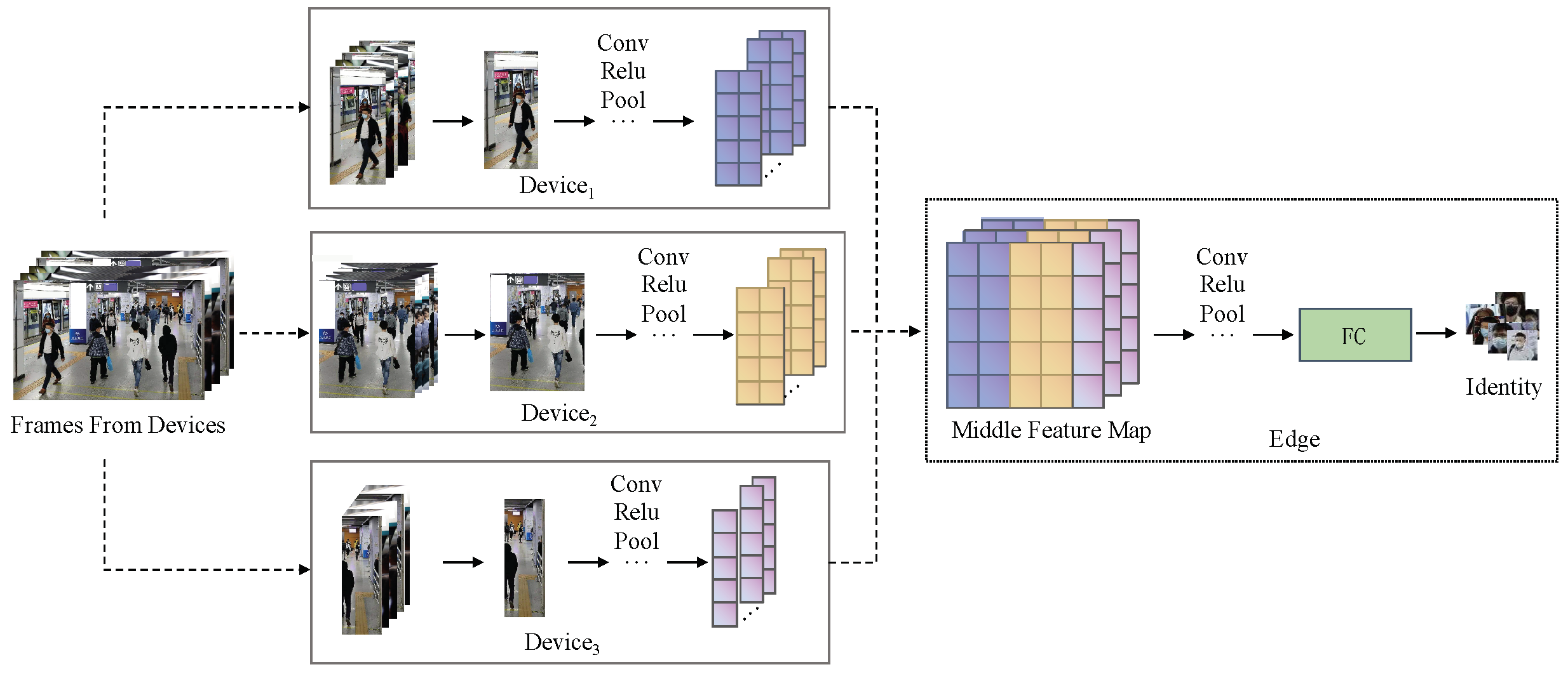
• We propose a distributed DNN inference framework (ADDP), which can dynamically and unevenly divide the computational tasks of DNN models according to the end-device computational capacity and network communication conditions, achieve parallel inference on multiple ends, and ensure the consistency of inference time across IoT devices as much as possible, in order to maximize the inference acceleration for DNNs and computational resource utilization for devices.
• We consider the continuous arrival of smart application data on the device and take the total inference time of the task as the optimization target. Instead of optimizing only the single DNN inference process, which is more in line with the actual application scenario, we share the edge’s computation task with the end device’s computation, effectively reducing the computation burden of the edge.
• We evaluate the ADDP to confirm its superiority by collaboratively reasoning for widely adopted DNN models on multiple devices in a real network. ADDP reduces single-frame response latency by 10–25% compared to the pure on-device processing.

The rest of the paper is organized as follows. Section 2 provides a summary of the literature related to our work. Section 3 proposes a regression model for predicting the computation time of DNN layers and models the problem of minimizing DNN inference latency. Section 4 describes the ADDP framework and the modules in it, and designs the methods for solving the collaborative inference strategy of DNN models in the smart city. Section 5 evaluates the effectiveness and convergence of the algorithm through experiments, and simulation results and analysis are presented. Section 6 provides a full-text summary.

2. Related Works

Intelligent applications’ collaborative inference approaches can be divided into collaborative execution between devices or between devices and cloud/edge. In this section, we briefly review the DNN model collaborative inference approach, summarize the shortcomings, and then show the advantages of ADDP.

2.1. D2D Inference

DNN collaboration among devices is divided into interlayer cooperation and intralayer collaboration. The devices in an interlayer cooperation must follow the original structure of the DNN and calculate successively. AAIoT [7] divided the DNN model under a multilayer IoT architecture with hierarchical constraint relations to achieve model collaborative inference for multiple devices. Hadidi et al. [8] proposed a partitioning algorithm that simultaneously performs on the data and model. Zhou et al. [9] designed a fusion search strategy based on dynamic planning, which adaptively performed layer fusion and thus dynamically distributed the workload according to the heterogeneity of resources to minimize the end-to-end inference latency. Based on the compatibility between the multilayer structure of a DNN and mobile edge computing (MEC), He et al. [10] deployed the model to multiple devices in a layered structure by optimizing the device resource occupancy and realized the distributed inference of DNN. The data transmission delay, processing delay, and queuing delay were integrated and optimized.

CoEdge [11] considered computational and communication resources and used layer fusion combined with a workload dynamic adjustment mechanism to achieve load balancing on heterogeneous devices. Ren et al. [12] proposed a collaborative approach in order to fully utilize 5G resources, which could perform fine-grained DNN elastic computational partitioning, and deployed the model on multiple end devices, as well as on the cloud and edge, to achieve collaborative inference, and finally developed a mobile Web AR application to verify the effectiveness of the method. EdgeSP [13] designed a multiple-fused-layer-block parallelization strategy to reduce the communication overhead between devices during parallel inference, effectively reducing the average task inference delay, and improving resource utilization by adding early exit branches. Jouhari et al. [14], in order to achieve inference of complex DNN models by unmanned aerial vehicles (UAVs) while avoiding air- and ground-generated additional communication delays, proposed a method for a dynamic collaborative DNN model inference by UAV air-to-air communication, which improved the real-time DNN inference while effectively utilizing the storage and computational resources of UAVs. DEFER [15] proposed a distributed edge inference framework to partition the model and perform distributed inference on resource-constrained devices, effectively reducing the device energy consumption.

2.2. D2C Inference

The end-to-end collaborative cloud execution of DNNs for model inference is achieved by offloading some of the DNN model computation tasks. Neurosurgeon [16] split DNNs in a chain topology with layer granularity by weighing the communication time and computation time based on the computation time required for different layers of the model and the size of the data generated. DDNN [17] proposed a distributed deep neural network that collaborated with end devices, edge devices, and central servers to achieve distributed inference and designed early exit branches to avoid the need for servers to reason about simple inputs, effectively improving the performance of the model on IoT devices with limited resources. To minimize the computation, IONN [18] considered that servers did not necessarily store models that needed to be offloaded and constructed the model offloading process and inference process as a directed acyclic graph (DAG). IONN solved the optimal offloading policy by solving the shortest path of the DAG while avoiding the unnecessary model structure deployed on the server. This method of solving the optimal partition by constructing a computational graph has received much research attention. JointDNN [19] considered the problem of solving multiple cut points by constructing the graph with the computation time of the layer as the node and the data transfer time was used as the edge, with energy, latency, QoS, battery consumption, and cloud server blocking as constraints to obtain the offloading strategy for multiple cut points of the DNN model, by solving the shortest path from input to output. Edgent [20] adaptively sliced the DNN model based on the available bandwidth between the edge server and the end device to offload more computations to the edge server at a smaller cost of transmission delay, thus reducing both data transmission latency and model computation latency. To avoid suboptimal solutions due to prediction errors in the execution time of each layer of the model, ANS [21] learned by observing the delay and used a contextual gambling machine to predict the optimal cut point.

Dyno [22] raised the priority of key frames to provide differentiation for different data in the learning process. D3 [23] proposed a dynamic DNN decomposition system for synergistic inference without precision loss. A regression model was used to estimate the processing time of DNN layers. The interlayer cut using HPA (heuristic method) was used to achieve collaborative inference at the cloud edge, and the feature maps of the convolutional layers were spatially split into blocks using a vertical separation module, allowing the convolutional layers to execute in parallel at the edge nodes.

3. Preliminary

We aim to build a distributed DNN partition framework to accelerate the inference process of dynamic video streams on resource-limited devices, where the way to create the feature map and model cut allocation, memory footprint, and model computation overhead are the key factors considered. Thus, we further investigated the following two aspects.

3.1. Hierarchical Prediction Model

The model ran on a single device, and the model inference time only included the computation time of the model. When multiple devices are used for collaborative inference, the time required for data transfer between devices also needs to be considered to achieve collaborative inference, and a suitable model allocation strategy needs to be chosen to take the time to get the model prediction results shorter. Therefore, the computation time of the model needed to be modeled, while the output data volume was recorded to calculate the transmission time.

As shown in Figure 2, the model inference time is mainly composed of three parts: end computation time, communication time, and edge computation time. We set 22 candidate cut points for ResNet18. The reasoning process on both sides of the cut point was performed on the terminal device and the edge device, respectively, and the communication time depended on the size of the feature map. Therefore, the model inference time varied with the location of the cut point. We tested and counted the results of different split point selections on a Raspberry Pi and a laptop with Intel CPU chips.

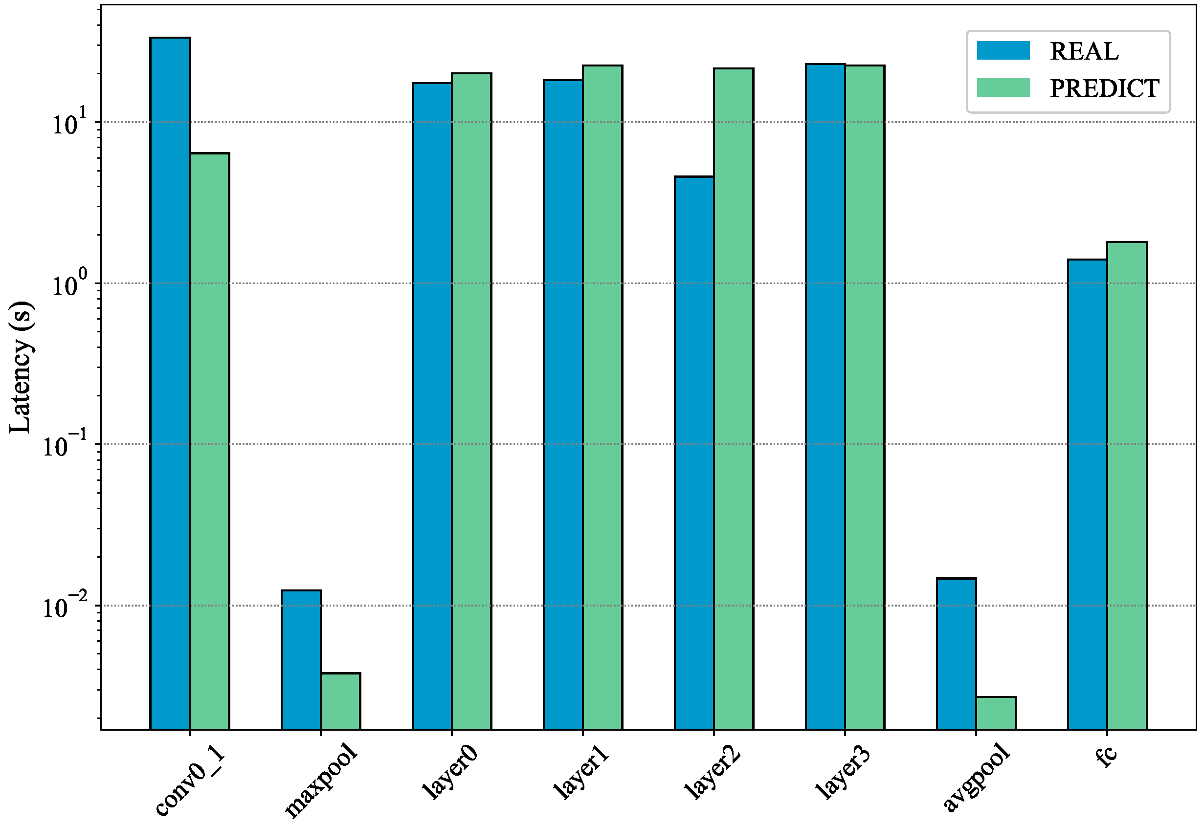
3.1.1. Estimation on Inference Delay

In the process of collaborative device inference, the model partitioning configuration relies on the accurate estimation of the model inference time. Methods exist to execute DNN models online and determine the inference time; however, due to the dynamic nature of idle computing resources, it is time-consuming and inaccurate to execute each layer and count the inference time on end-devices and edge servers. To solve this problem, we used a regression model that considered the allocatable computing power of devices with DNN parameters to estimate the inference time of each layer of the DNN. The DNN parameters included the data dimension and arithmetic type of each layer. According to Roofline [24], the inference time of the DNN model mainly comes from floating-point operations (FLOPs) and data access. The FLOPs are mainly present in the convolutional layer, fully connected layer, normalization layer, etc. They are related to the input size, the number of neurons, and step length. The data access process is prevalent in each layer of the DNN and is related to the data size. The DRAM Traffic (DT) is the size of bytes required to access the storage unit during the model computation, which reflects the model’s demand for storage unit bandwidth. In access-intensive operators such as ReLU, Concat, etc., access traffic significantly impacts the model inference time.

Specifically, we defined the theoretical computational peak of device $D_i$ as $F_i$ and the maximum memory bandwidth as $MM{B}_i$. The height, width, and number of channels of the input and output data were defined as $H_{in},W_{in},C_{in},H_{out},W_{out},C_{out}$, respectively. For convolutional layers, the FLOPs are also related to the step size s and the size K. For computationally intensive operators, the computation can be expressed uniformly as $FLOPs=H_{out}·W_{out}·C_{in}·K^2·C_{out}$. For the access-intensive operator, the computation is negligible, and the DT can be expressed as

$$DT=\alpha ·H_{in}·W_{in}·C_{in}+\beta ·H_{out}·W_{out}·C_{out}+\gamma ·C_{in}·C_{out}·K^2.$$

(1)

The values of $\alpha ,\beta$, and $\gamma$ represent the number of times each operator needs to access the input, output, and operator data (such as convolution kernel) during the calculation process. The details are shown in

Table 1. The operator data traffic reference.

-	$\mathit{\alpha }$	$\mathit{\beta }$	$\mathit{\gamma }$
Conv	1	1	1
FC	1	1	1
Norm	1	1	0
Pool	1	1	0
ReLU	1	1	0
Concat	2	1	0
EltWise Add	2	1	0

.

We modeled the regression for the computation time of each layer in DNN with $F_i$, $MM{B}_i$, $FLOPs$, and $DT$ as input parameters. The inference time can be expressed as

$$T_{infer}=Func(F_i,MM{B}_i,FLOPs,DT).$$

(2)

We tested the model inference latencies for all layers on the ResNet family of feature extractors, including inputs of different lengths in the W dimension. Figure 3 shows that the actual processing time of our proposed regression model is similar to the predicted processing time.

3.1.2. Estimation on Communication

During collaborative device inference, the intermediate data cross-device transfer time affects the device parallelism and thus the overall inference latency. The cross-device transfer time is related to the data size and the network bandwidth $B_{i,j}$, which is monitored by the analyzer on each device. The intermediate piece of data is the output feature map from the model cut points, and the size of the feature map is jointly determined by $H_{out},W_{out},C_{out}$. The transfer time can be calculated by the following equation.

$$T_{trans}=\frac{L_{out}·W_{out}·C_{out}}{B_{i,j}}$$

(3)

3.2. Optimization Model

A total of m devices perform the same task with an inference model of n layers for that task. The terminal device $D_i$ has a task $Tas{k}_i$ with task size $P_i$. The total inference time $T_{total}\sim O(T_{computation}+T_{communication})$ of the model for the collaborative completion of $Tas{k}_i$ between devices without considering the tasks on other devices. Because the inference process of the model is limited by the sequential structure of the layers, when multiple devices perform the same layer in concert, the required input may be partially present on other devices. Therefore, the device $D_j$ needs to wait for the required input data to be inferred or transferred to $D_j$ when reasoning about the lth layer of the model.

We aimed to build the inference latency of all tasks on multiple ends with respect to the communication bandwidth, the layer where the cut point was located, and the quantity of data to be processed by the device, and to minimize the total inference latency of the DNN model through edge-end collaboration. Specifically, for a DNN model, the DNN logic layers in the model were used as edges to construct the computational graph, assuming a total of n layers in the model, and a unique identifier $v_k^l$, where $v_k\in \mathbb{D}\cup \mathbb{E}$, was set for the lth layer in the device $v_k$ according to the order of execution of the logic layers. Then, according to the data dependencies between the DNN layers, the relation $(v_i^l,v_j^{l+1})$ was defined as the edge $e_{i,j}^l$ when the output of the device $v_i$ layer l was used as the input of the device $v_j$ layer $l+1$. All the logical layers of the DNN model $v_1^1,v_1^2,\cdots ,v_m^n$ and the data association between the logical layers were used to construct a DAG $\mathcal{G}=(\mathcal{V},\mathcal{E})$ as shown in Figure 4, where $\mathcal{V}=v_1^1,v_1^2,\cdots ,v_m^n$ represents the vertices of the graph, and ${\mathcal{E}}^l\subset {\mathcal{V}}^l\times {\mathcal{V}}^{l+1}$ represents the data dependencies between adjacent DNN layers.

We used ${tv}_k^l$ to denote the inference time of the model on layer l on the end device $v_k$ as the weights of all vertices in the DAG. For node pairs with data dependencies $(v_i^l,v_j^{l+1})$, we used ${te}_{i,j}^l$ to denote the transmission time of data between devices as the weights of all edges in the DAG. The weights of different edges varied greatly, and the data transfer on the same device was achieved through memory access, which was much smaller than the transfer time between devices and therefore negligible, with the constraint ${te}_{i,i}^l=0$. The transfer time between end devices was smaller than the communication time from end devices to edge servers with the constraint ${te}_{i,k}^l>{te}_{i,j}^l,\forall v_i,v_j\in \mathbb{D},\forall v_k\in \mathbb{E}$.

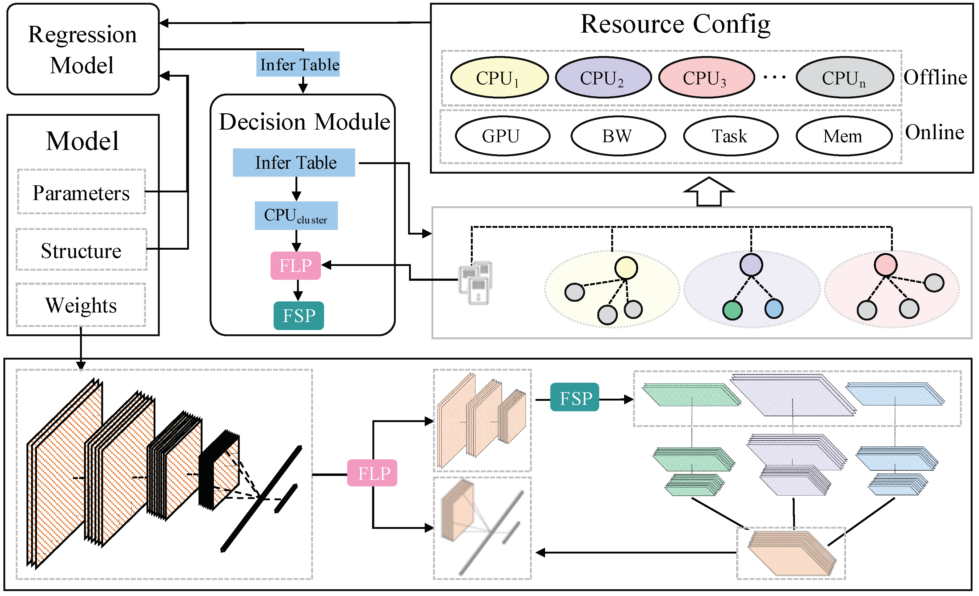
4. The Proposed ADDP Framework

4.1. Framework Overview

Figure 5 depicts the DNN collaborative inference acceleration using ADDP. Currently, ADDP supports two major existing feature extraction networks, including the VGG and ResNet families. In this section, the task and device situation in a smart city scenario is described with the various modules of the framework and the data flow between them. The specific model cutting algorithm is introduced in the next part of this section.

Device topology and tasks. There are many devices and a high task complexity in a smart city, which cannot be done in real-time by end inference. Although the computational resources at the edge are richer than those at the end devices, completing the entire inference process at the edge cannot satisfy the real-time response constraint of each task. Edge–end collaboration, as a method that can effectively utilize the computing resources of devices and expand the total computing capacity while guaranteeing the inference delay, is the best technical means to process data in the smart city in real-time. We analyzed the best way to provide intelligent services for smart city stations based on the high number of cameras and uneven distribution of pedestrian density and devices. The distribution characteristics of smart city devices and pedestrian flow cause differences in the quantity of data collected by the devices. The quantity of data collected by devices distributed near dense crowds is greater than that collected by devices in other locations, but the computing power of the devices is fixed. Therefore, the best technical means to process data in a smart city in real-time is to reason in parallel between devices and then collaborate with the edge. For a smart city, 1-to-N technology can realize the carrier technology of this model’s reasoning method. The devices are able to communicate with each other, the data volume can be balanced, and the devices can be aggregated into one computing node from the physical connection, and then the edge–end collaboration is carried out.

Resource config. We abstracted the resource information of the device and the network condition into static offline and dynamic online configurations. Offline resource information includes the CPU information of all end devices and measures the computational power in the subsequent process without further change. Online updated resource information includes the edge information, such as GPU arithmetic power, disk capacity, memory size, the quantity of data collected on each device, and the bandwidth. Offline and online resource information are both used as configuration information and input to the regression model to predict the inference time of each layer of the DNN model.

Regression model. Based on the resource information of the device, we applied the method of Section 3 to predict the computation time of each layer of the DNN model. We also dynamically adjusted the prediction results according to the changes of online resource information in resource config to ensure the optimal prediction of the decision module’s results to the maximum extent. The regression model sends the generated infer table to the master node and edges involved in the resource config.

DNN model. This part includes parameters, structure, and weights. Parameters describe the type of operators used in the DNN model, the size of the operators, and the data dimension. Structure stores the DNN model computational graph and data flow. Weights hold the parameters necessary for the model to be computed during the inference process and are only loaded during the model inference process.

Decision module. The decision module determines the selection of the model split points, which is the core part of the ADDP framework, including two main modules, feature-map layer partition (FLP) and feature-map size partition (FSP). First, the edge allocates resources to the task requests of each master node through FLP according to the received infer table, which is expressed as the decision of the horizontal splitting point of each model. The master node then inputs the infer table into the FSP and decides the number of tasks each device should compute in the cluster based on the received horizontal partitioning policy. The specific task cost is quantified by the size of the data that each device should process. Finally, the input size table required for each device in a single data inference is downlinked to all devices.

Distributed inference. The free computing resources of terminal devices and edge servers are dynamic, and we applied the FLP computing model by a layer strategy after converging network and resource characteristics. The quantity of data changes dynamically, and the amount of computation per data unit is constant. Applying the feature map partitioning strategy computed by FSP, we achieved the computational partitioning on the end device by balancing the computation per unit of data. Each device divides the data collected by the device according to the input size table issued by the master node. The segmented input data are then transferred to the corresponding device. After a device finishes inference, it uploads the inference results to the edge for subsequent model inference.

Application in Video Stream. Next, we explain how ADDP works on large-scale video streams with an object detection application as an example. In a smart city, an AI camera deployed with an object detection application captures a live video stream and selects some frames for further detection. For data collection devices in the same region, the FSP module develops a segmentation policy for each frame based on the device’s arithmetic power and assigns the segmented patches to the corresponding devices in the region. FLP is responsible for formulating the partitioning strategy of the feature extraction backbone network in target detection, and the master node must choose a model partition point to collaborate with the edge server. The edge server updates the model partition point by gaming with the connected master node. After inference is completed, the object detection results (i.e., object bounding boxes and class labels) are recorded into the video. It is worth noting that to better apply to dynamic video streams, the AI camera and edge server rely on the contextual relationship of the video stream. For example, when new objects or scene changes appear in the video, key frames (containing important targets or events) may appear in the video stream. The presence of key frames increases the density of camera data acquisition, which affects the partitioning settings of data and target detection models.

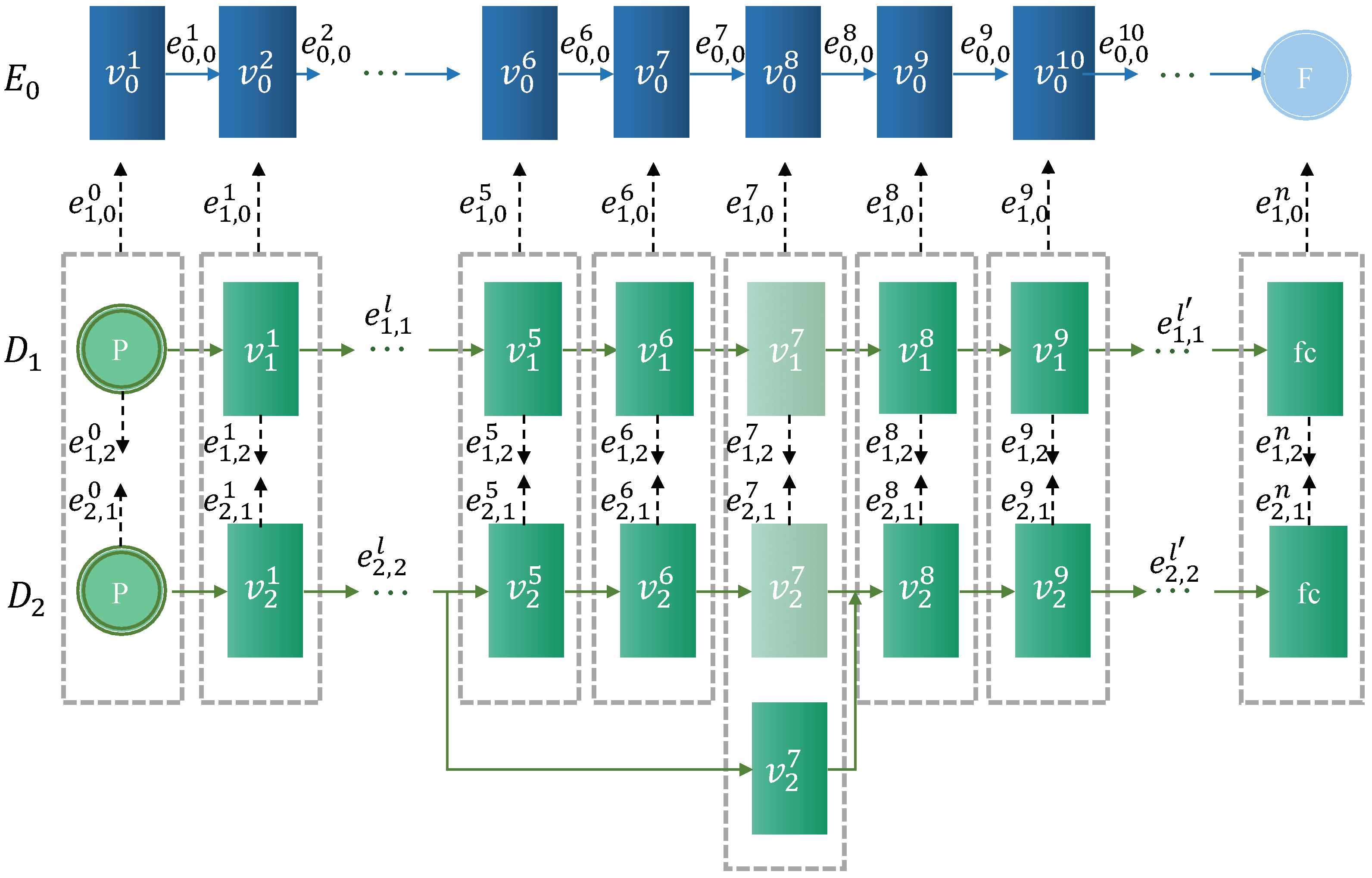
4.2. The Horizontal Partition between the Devices Cluster and the Edge

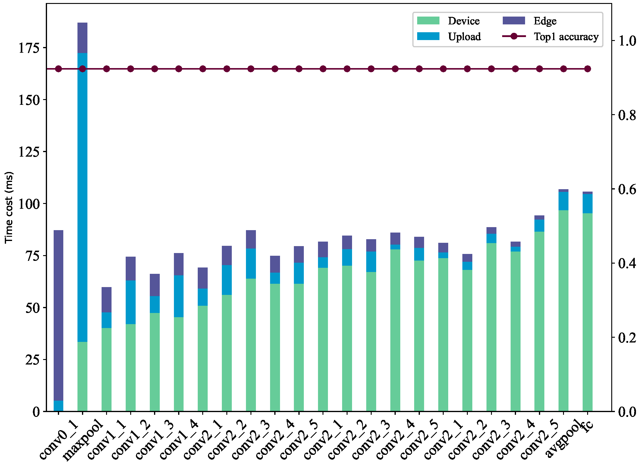
4.2.1. DNN Model Cut-Point Setting

We used computationally intensive operators as feasible model cut points, such as convolutional layers, pooling layers, etc., and the remaining as additional layers to the closest computationally intensive layers. For example, the convolutional layer in a common DNN was immediately followed by a ReLU, which we no longer regarded as a potential division point, but it was executed on the same device along with the conv. In particular, for models with a nonchain structure, such as ResNet18, the residual block structure internally, which will be executed in order of model succession, can be converted into a practically chained structure, at which point the selection of cut points can be unified.

4.2.2. Multidevice Single-Edge Cut-Point Solution

In a multidevice single-edge smart city scenario, the cut-point configuration chosen by the master node of each terminal cluster affects the computing power allocation of the edge server. In this case, it is not beneficial for the terminal device clusters to monopolize the server resources. Due to the arithmetic capacity of different device clusters, there are differences in the quantity of data collected. Therefore, different device clusters have various pursuits for DNN model cutting points. Game theory is a powerful tool for designing distributed mechanisms that enable end devices to make decisions that satisfy other terminals and servers in the face of the DNN model and achieve the shortest average response time for all tasks. Game theory provides a practical framework to analyze the interactions between multiple clusters of devices that act in their interest and to design incentive-compatible mechanisms for remote execution of parts of the model so that no endpoint has an incentive to deviate unilaterally.

Specifically, we modeled the model cut-point solution problem between camera sets and edge servers in a smart city scenario where an AI camera 1-to-N technology was deployed as a multiuser cut-point game. Based on this, a distributed cut-point updating algorithm was proposed to achieve the Nash equilibrium of the game. In Algorithm 1, we set the DNN model on device $D_i$ to execute all remotely, i.e., $partition\left(0\right)=end$. Each node cluster then interacted with the server to obtain the latest resource allocation information and made a cut-point update request, iteratively improving its own partitioning decision, which had impacts on all devices and could reach the optimal global solution in a finite number of times. The $D_i$ cut point $partition\left(t\right)=i$ at moment t, and the three parts of DNN model time overhead returned by the server were $T_j^i,T_e^i,T_{j,e}^i$. Based on the server inference time delay $T_e^i$, $partition\left(t\right)$ and the regression model, we could estimate the arithmetic power $F_e$ that can be allocated to $D_i$ by the time slot t server. Based on the computational resources $F_i$ of $D_i$, the communication bandwidth $B_i$, the available server resources $F_e$, and the model parameters, we found the optimal cut point $partition(t+1)$ that applied to this case. $D_i$ sends an update request to the server. If the server allows it, $D_i$ adjusts the cut point. Otherwise, the cut policy remains unchanged.

Algorithm 1 Distributed partition decision algorithm

initialization: each device cluster $D_i$ chooses the partition decision $partition\left(0\right)=end$ end initialization: 1: for each device cluster and each decision slot t in parallel do 2:  Execute the first $partitio{n}_i\left(t\right)$ layer of the DNN model 3:  Receive the inference time $T_e^i$ and data transmission time $T_{j,e}^i$ 4:  Estimate the computing power $F_e$ that the edge server can allocate to $D_i$ 5:  Compute the optimal updating $partitio{n}_i(t+1)=Func(F_i,B_i,F_e,cfg)$ 6:  if ${\Delta }_i(t,t+1)\ne 0$ then 7:   Send RTU request to the s for contending for the partition update opportunity 8:   if receive the permission from s then 9:    Update the configuration of the device $D_i$ in the next time slot $partitio{n}_i(t+1)$ 10:   else 11:    Keep the original partition configuration $partitio{n}_i(t+1)=partitio{n}_i\left(t\right)$ 12:   end if 13:  else 14:   Keep the original partition configuration $partitio{n}_i(t+1)=partitio{n}_i\left(t\right)$ 15:  end if 16: end for

The server $S_i$ executes the computation tasks for all end-device offloads as a task queue and returns the time from the start of the offload until the server gets the result $\{T_e^i,T_{j,e}^i\}$ for the corresponding task. For $partition$ update requests from n end devices, only one is granted at a time (one is randomly selected to return a permit), and after a finite number of time slots, the system can reach a balanced state.

4.3. Device Intracluster Feature Map Division

After determining the cut point between device clusters and edge servers, the model inference tasks per unit of data need to be distributed within device clusters by end-device computing power. We used a DNN vertical segmentation method divided by feature maps.

4.3.1. Overlap Area Calculation

In DNN architectures, multiple convolutional layers are usually stacked together as the feature extraction part. In such DNNs, each data element of the feature map in the intermediate layers depends on a local region in the input feature map. Therefore, we can decompose the DNN computation task by partitioning the region of the input feature map. In recently popular backbone networks such as Resnet, DNNs are usually divided into blocks composed of multiple convolutional layers and connected by a skip-connection. Due to the branching structure, the mapping relationship of regions connected across blocks in Resnet is more complicated than that of traditional backbone networks.

Unlike the grid decomposition in Deepthings [25], this paper used a feature-map-partitioning method in W dimensions, i.e., strip partitioning. The strip segmentation is easy to scale and can reduce the overlapping area. The local area size is related to the receptive field of each output data element, and the receptive field (RF) can be calculated by the following equation

$$R{F}_{l+1}=R{F}_l+(K_{l+1}-1)·\prod _{i=0}^{l}strid{e}_i·dilatio{n}_{l+1}.$$

(4)

The $K_{l+1}$ denotes the convolution kernel size of the ($l+1$)th layer and $R{F}_0=1$. After calculating the receptive field, the mapping area of the output feature map region in the input feature map can be calculated based on the receptive field. For any selected column data $X_{out}$ in the output feature map, its corresponding input column $X_{in}$ can be written as:

$$X_{in}\triangleq \prod _{i=0}^{l}strid{e}_i·X_{out}\pm \lfloor \frac{R{F}_{l+1}}{2}\rfloor .$$

(5)

When the cross-layer connections are deeper, the RF is more extensive, and there is considerable overlap between the input regions required for each region of the output feature map. There are two ways to cope with these overlaps. The first is to communicate and fuse each layer to avoid overlaps. Unfortunately, this approach introduces a significant communication overhead and can significantly reduce the parallelism of collaborative inference because of the waiting for each other. The second approach is to cut the data directly based on the computed overlap region size, which introduces additional computational overhead but improves parallelism. We adopted the second approach and propose an improvement of the padding approach.

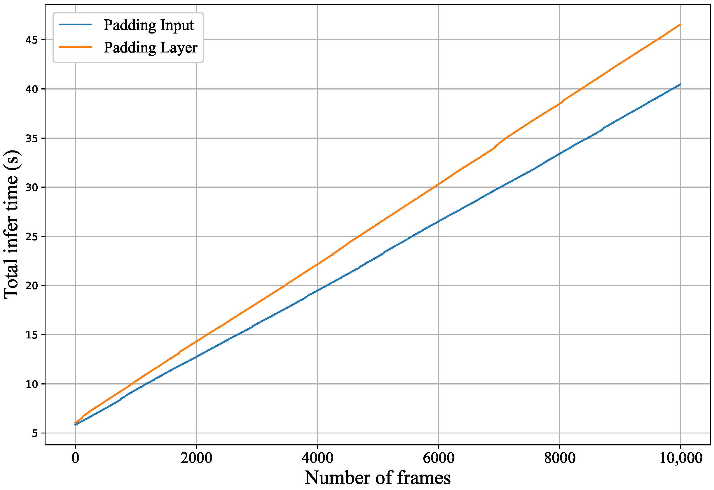
4.3.2. Tensor Padding Optimization

When the convolution kernel size is larger than one, the conv operator relies on the padding of the output tensor. When there is an overlap between cross-layer region mappings, we must design a reasonable padding strategy to maintain the model’s original accuracy. Take the tensor $x_{out}^0$ in dimension W of the output feature map as an example, its mapping region on the input feature map is $\{x_{in}^0,x_{in}^1,\cdots ,x_{in}^n|n={\prod }_{i=0}^l·x_{out}^0+\lfloor \frac{R{F}_{l+1}}{2}\rfloor \}$. At this point, the left region should be padding n columns.

We designed two types of padding implementation. The first one was layered padding, in which the position and number of columns to be padded were judged at each layer, and a tensor padding operation was performed. Since there was a logical judgment, layered padding extended the computation time of each layer. The second type was input padding, and the corresponding number of tensors were padded directly on the output feature map based on RF. Since the input size was increased, it also affected the model inference latency. The comparison of the two padding methods is indicated in the subsequent experiments.

Due to the branching structure in the backbone network, the sensing field of the main data stream was different from that of the skip-connection, so it was necessary to set different padding sizes during the operation. In the face of such a branch structure, Equation (5) was still applicable. Depending on the RF size, different padding configurations can be set for various branches.

4.3.3. Data Segmentation

In order to improve the parallelism of all devices within a device cluster, it was necessary to divide the computational tasks per unit of data according to the actual computational capacity of the devices. Different devices within the same cluster capture different quantities of data, which can be seen as all devices jointly processing the captured video frames by a model vertical partitioning technique based on feature map partitioning. For example, in a device cluster with n devices, where device $D_i$ acquires $P_i$ frames per unit time, the device cluster can be regarded as acquiring ${\sum }_i{P}_i$ frames of data per unit time. We only needed to divide each data frame assigned to these n devices according to the actual computational speed of $D_i$. Based on the regression model built in Section 3, we could estimate the inference time of devices at each input data size to search for the partitioning configuration that minimized the variance of inference time for all $D_i$. However, this search approach had a significant time overhead, prolonging the inference time delay. DeepSlicing [26] demonstrated that the input data size on the slice dimension was roughly proportional to the inference latency of multiple consecutive layers in a DNN. Therefore, we directly sliced the input data on the W dimension based on the ratio of device arithmetic power, achieving near-optimal device parallelism.

5. Performance Evaluation

In this section, we compare FLP and FSP in ADDP with the current model-cutting methods to verify their performance.

5.1. Experiment Settings

We built a combined simulation and hardware testbed to validate the ADDP design and evaluate its performance for video-streaming object detection applications. We used four Cortex-A72-processor-equipped Raspberry Pi 4s with onboard cameras as end devices. We connect the Raspberry Pi to a common switch without limiting the network transmission speed to simulate the communication conditions between the end devices in a real application scenario. The edge server was simulated using a laptop equipped with a 2.6 GHz Intel Core i7 chip.

In addition, limited by the hardware cost, we simulated the game process between one server and dozens of AI cameras regarding the model-partitioning strategy by numerical simulation. Three state-of-the-art DNN models that are often used as object detection backbone networks, namely Vgg16, ResNet18, and ResNet50 were considered in the experiments. We implemented the ADDP framework based on PyTorch and OpenCV, performed partitioning strategies, and ran deep inference on these models. We evaluated the cutting method by the inference time of feature extraction models commonly used in computer vision applications. The layer completion time was the time from the start of DNN inference to the completion of that layer, and the completion time of the last layer was the total completion time of that model.

Three model-level partitioning methods were chosen as the baseline of comparison for FLP.

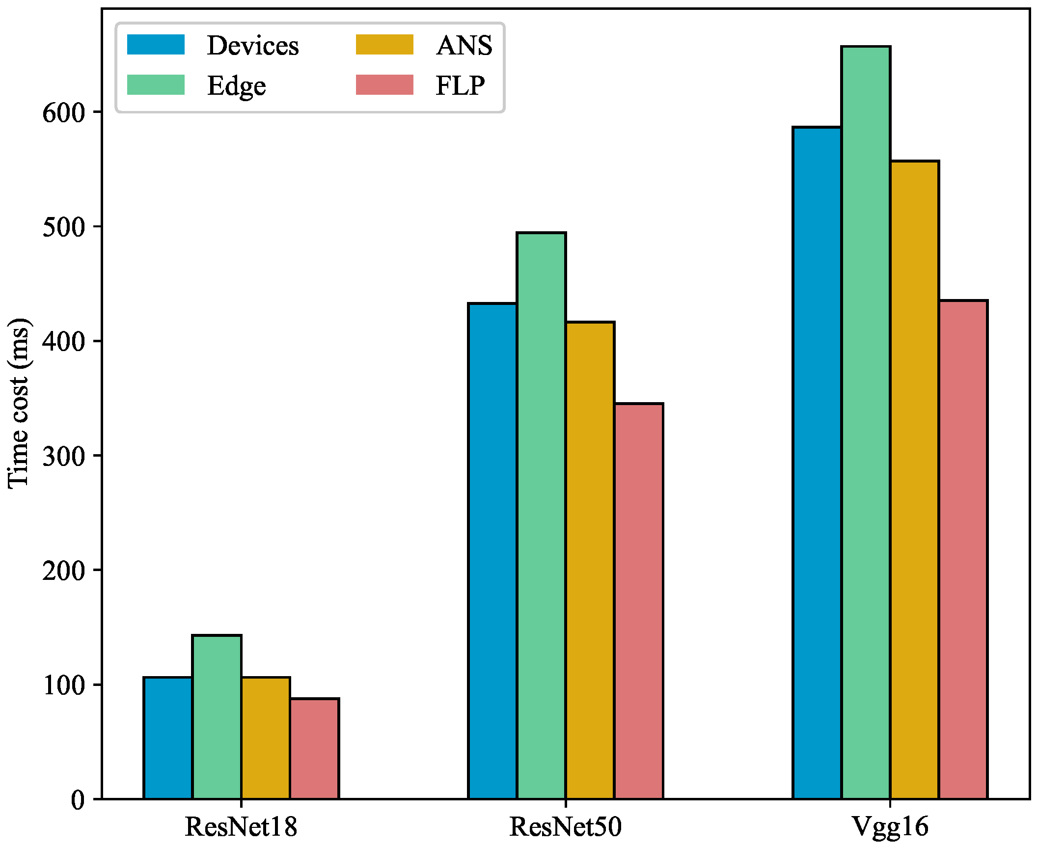
• Devices: all layers of the DNN model were executed on the terminal cluster, i.e., the cut point was set to the maximum value of the corresponding model.
• Edge: DNN models of all access devices were executed on the edge server, i.e., the cut point was set to 0.
• ANS [21]: a built-in online learning module was used to search for the best cut point based on a novel contextual slot machine algorithm to generate partitioning decisions dynamically.

We selected three model vertical partitioning methods as the baseline for comparison of FSP.

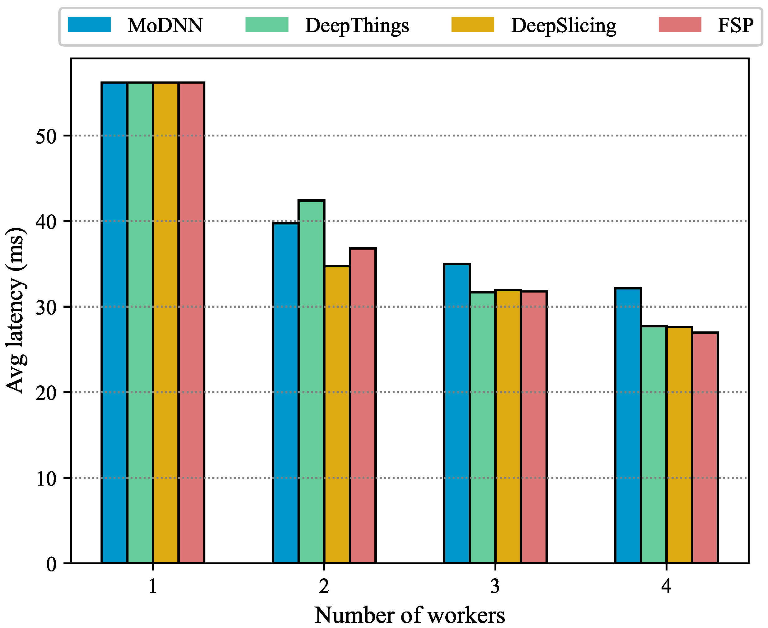
• MoDNN [27]: based on the characteristics of convolutional layers with computational consumption and fully connected layers with storage consumption, a differential intralayer partitioning approach was performed for different types of DNN layers, the sliced feature map was assigned to multiple devices for collaborative computation, and finally the output on each computational node was collected by the master node for the next layer of inference; the process introduced a significant communication overhead.
• DeepThings [25]: end-to-end slicing of the chain structure of the model, using layer fusion, divided the feature map process into multiple independent parallelizable computational tasks, reducing the quantity of data that needed to be communicated, and avoiding overlapping computation between adjacent task partitions by fusion slicing (FTP) method and task assignment strategy.
• DeepSlicing [26]: for the shortage of MoDNN and Deepthings, the single feature map was sliced according to bars to reduce the part of repeated computations, balanced single-layer slicing and multilayer vertical slicing, and the number of compromises was used to reduce the duplicated region of feature map and not to divide the parallel computation tasks too much.

5.2. Results

5.2.1. End-to-End Inference Delay

Figure 6 shows the inference latency comparison of three horizontal segmentation baseline algorithms with FLP on different DNN models. The input data were generated on four access devices, the edge server used a GPU, and the transmission rate was fixed to 100 Mbps. It can be seen that the inference latency of Edge is higher than Devices because Devices is a device cluster including four devices with specific arithmetic capacity. There is also an additional time cost for clusters of devices to upload data to the edge servers. ANS and FLP are able to make an effective trade-off between on-device processing and edge offloading, thus achieving better results than Edge and Devices. FLP is based on the ADDP framework and has parallel optimization for local device processing and a reasonable cut-point selection, resulting in less transmission latency than ANS, which is more prominent for the more complex DNN.

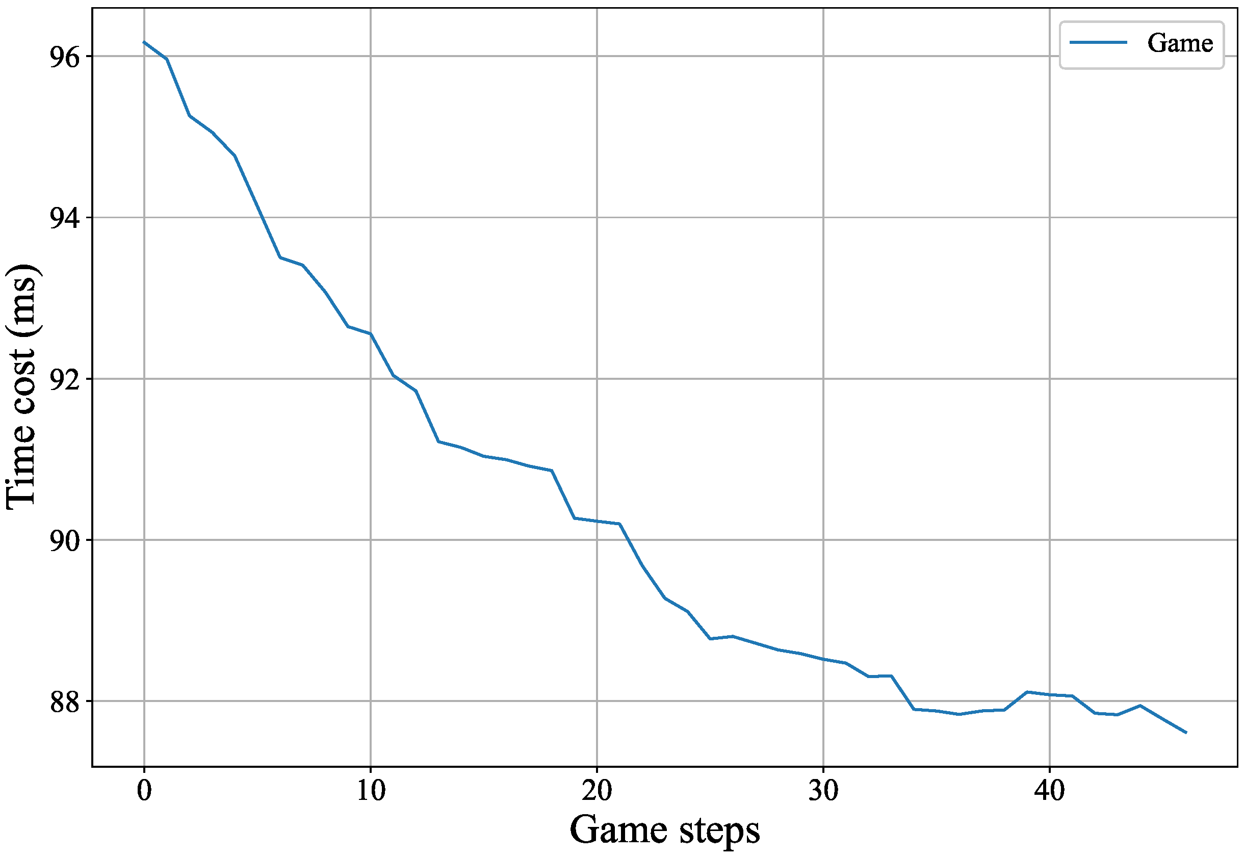
5.2.2. Delayed Changes in the Gaming Process

In the FLP module, the initial cut point of the model was obtained based on a regression model of the execution time of each layer of the model and the assumption of equal sharing of edge server resources. However, this cut-point method had a higher inference delay than the optimal cut point. Figure 7 shows the variation of the average inference delay during the game based on the FLP module for all access devices. With dozens of access device clusters, FLP used the game between master nodes to continuously adjust the model cut points and reach the equilibrium state in a limited time. The equilibrium state horizontal cutting strategy reduced the DNN model inference time overhead by about 6% compared to the heuristic cutting method.

5.2.3. Comparison of Feature Map Segmentation Methods

The first half of the DNN model in the horizontal cut was executed distributively inside the device cluster. Figure 8 shows the average inference latency of the three vertical partitioning methods based on feature map partitioning for the different number of devices. Overall, within a device cluster, FSP performs better compared to other feature map partitioning methods. This is due to the strong adaptability of the FSP algorithm to DNN networks with branching structure and optimization of the input feature maps. MoDNN suffers from the effect of different devices waiting for each other and has the lowest parallelism and, therefore, the highest average latency. The two-dimensional feature-map-cutting method in DeepThings brings a larger overlapping region, and frequent overlapping data synchronization leads to the poorer performance of DeepThings than FSP. DeepSlicing has better memory and communication optimization, but the complex collaborative approach brings an extra burden when facing multiple devices collecting data simultaneously. Therefore, the additional cost increases as the number of workers increases.

5.2.4. Tensor Padding Time Cost

Figure 9 shows the cumulative time diagram on 10,000 input images at the edge server.

The straight-line slope in the figure represents the inference time delay of each image. It can be seen that the slope of the layered padding is significantly higher than the input padding, which is because the layered padding requires additional logic judgments between each layer in the DNN computation graph. These CPU-frequency-intensive logic judgments slow down the overall inference progress. Therefore, although the increase in feature map from padding the input data affects the inference latency, it still outperforms the hierarchical padding method.

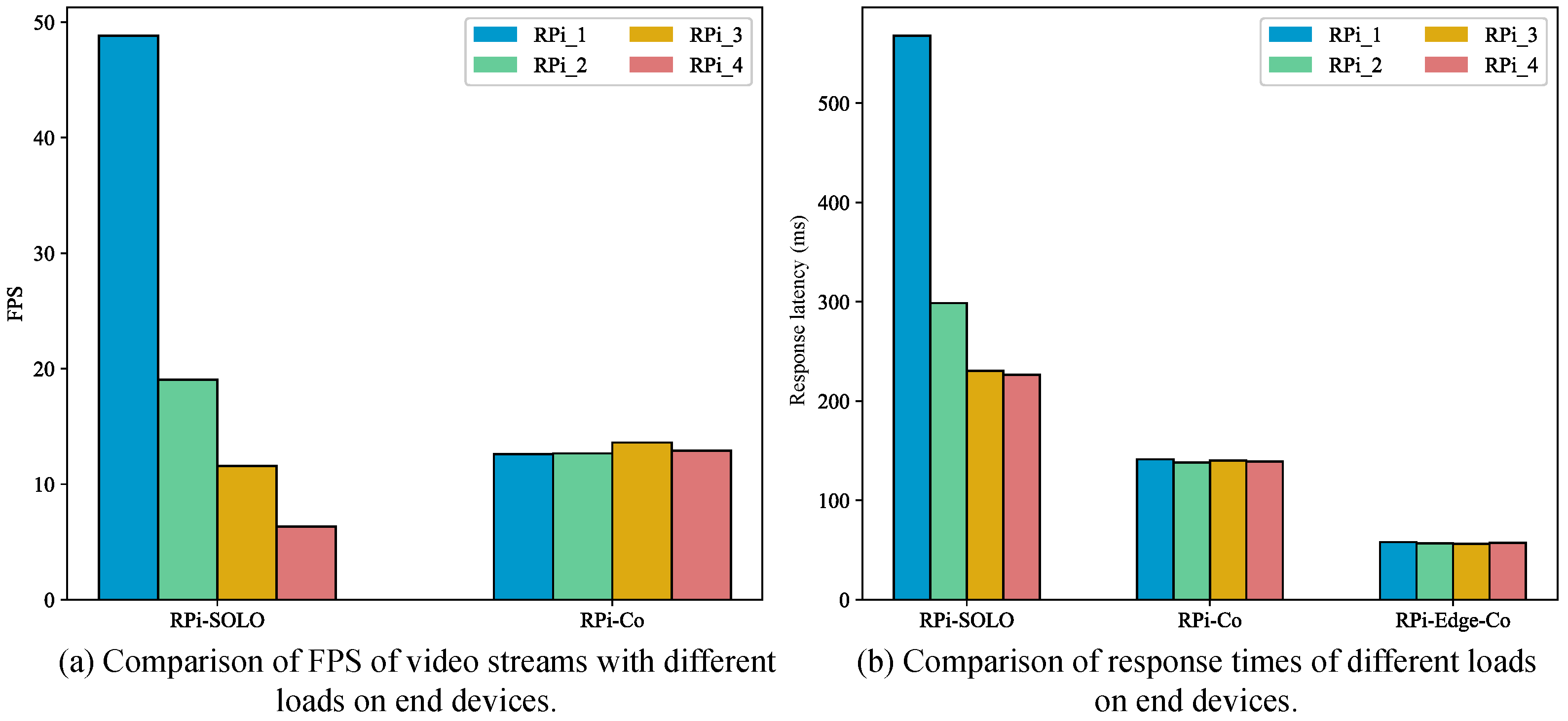
5.2.5. ADDP on Video Streaming

We tested the execution results of the object detection task under the condition of an unbalanced load of four intelligent cameras. The input video was captured by an onboard camera using OpenCV, and the video frames were captured at 1280 × 720 pixels, filtered, and converted to the size required by the DNN model: 224 × 224 × 3. We set up four Raspberry Pis with different crowd densities for 10 minutes of traffic video and filtered key frames by the interframe difference method to input into the target detection model. Among them, the larger the difference between frames, the more it meant that the frames could contain important objects or events. The video with a higher crowd density contained more key frames and a higher device load. The video key frame sampling rate and FPS are shown in the

Table 2. Execution statistics of 4 videos on Raspberry Pi.

-	Sampling Rate	FPS (ResNet18)	FPS (ResNet50)	FPS (Vgg16)
Video1	9.04%	48.81	32.86	10.77
Video2	23.18%	19.05	14.60	4.28
Video3	38.10%	11.58	8.27	2.79
Video4	69.87%	6.32	4.51	1.29

, in which all data come from the DNN inference statistics on the same Raspberry Pi. The FPS of the low-load (i.e., low key frame sampling rate) device is up to 48.8, reaching about eight times that of the high-load device.

After applying ADDP, the frame processing rate of each camera was determined and is shown in Figure 10; the FPS is the same for all devices, although the FPS of the low-load devices decreases. This is because the FSP divides the computation required for each frame after inputting it into the DNN model into four parts evenly, according to the device’s arithmetic power, so the load on each Raspberry Pi is the same, and it can be seen that the FSP module of ADDP ensures the consistency of inference time across IoT devices. In addition to FPS, the DNN models on different load devices have wildly different response times for key frames. We defined the key frame response time as the window size between acquiring key frames and getting the target frame. When the device is under high load, the pending frames are backed up into the input queue so that the key frame response time increases significantly. When FSP is applied, the response latency of all devices remains consistent and is lower than the result of a single device under minimum load. Each device is evenly responsible for a portion of the key frame area. The key frame response latency is further reduced to about 40% of the original one when FLP is combined with FSP because the model-partitioning module FLP arranges only the first three layers of ResNet18 to be executed on the four Raspberry Pi’s only, and the subsequent computations are executed in the simulated edge server. The experimental results show that our proposed solution can achieve consistency in inference time among the four devices with uneven load and reduce the critical frame response latency from 24.89% to 62.41% of the original latency through data division. Overall, ADDP reduces single-frame response latency to 10–25% compared to the pure on-device processing. Although not tested on a larger scale with real devices, the available experiments enable us to conclude that our proposed solution is applicable to dynamically changing video streams.

6. Conclusions

This paper proposed ADDP, an adaptive distributed DNN partition method that supports video analysis on large-scale intelligent cameras. ADDP has the following main characteristics and is suitable for large-scale equipment scenarios. The FLP module adopts a distributed decision-making technology to support model partitioning between the large-scale terminal equipment and edge servers. The FSP module supports multidevice data division, realizes the calculation division on the terminal device by balancing the calculation amount of the unit data, and supports the scene where multiple smart sensors collect data simultaneously. Experiments showed that ADDP was more efficient than the existing DNN collaborative inference framework, reducing the inference delay to 10–25% of that of the pure end-device processing on large-scale devices.

References

1. Maiano, L.; Amerini, I.; Ricciardi Celsi, L.; Anagnostopoulos, A. Identification of social-media platform of videos through the use of shared features. J. Imaging 2021, 7, 140. [Google Scholar] [CrossRef] [PubMed]
2. Zhou, S.; Tan, B. Electrocardiogram soft computing using hybrid deep learning CNN-ELM. Appl. Soft Comput. 2020, 86, 105778. [Google Scholar] [CrossRef]
3. Cicceri, G.; De Vita, F.; Bruneo, D.; Merlino, G.; Puliafito, A. A deep learning approach for pressure ulcer prevention using wearable computing. Hum.-Centric Comput. Inf. Sci. 2020, 10, 1–21. [Google Scholar] [CrossRef]
4. Zhou, Z.; Chen, X.; Li, E.; Zeng, L.; Luo, K.; Zhang, J. Edge intelligence: Paving the last mile of artificial intelligence with edge computing. Proc. IEEE 2019, 107, 1738–1762. [Google Scholar] [CrossRef] [Green Version]
5. Ouyang, T.; Zhou, Z.; Chen, X. Follow me at the edge: Mobility-aware dynamic service placement for mobile edge computing. IEEE J. Sel. Areas Commun. 2018, 36, 2333–2345. [Google Scholar] [CrossRef] [Green Version]
6. Cevallos Moreno, J.F.; Sattler, R.; Caulier Cisterna, R.P.; Ricciardi Celsi, L.; Sánchez Rodríguez, A.; Mecella, M. Online Service Function Chain Deployment for Live-Streaming in Virtualized Content Delivery Networks: A Deep Reinforcement Learning Approach. Future Internet 2021, 13, 278. [Google Scholar] [CrossRef]
7. Zhou, J.; Wang, Y.; Ota, K.; Dong, M. AAIoT: Accelerating artificial intelligence in IoT systems. IEEE Wirel. Commun. Lett. 2019, 8, 825–828. [Google Scholar] [CrossRef]
8. Hadidi, R.; Cao, J.; Woodward, M.; Ryoo, M.S.; Kim, H. Distributed perception by collaborative robots. IEEE Robot. Autom. Lett. 2018, 3, 3709–3716. [Google Scholar] [CrossRef]
9. Zhou, L.; Samavatian, M.H.; Bacha, A.; Majumdar, S.; Teodorescu, R. Adaptive parallel execution of deep neural networks on heterogeneous edge devices. In Proceedings of the 4th ACM/IEEE Symposium on Edge Computing, Arlington, Virginia, 7–9 November 2019; pp. 195–208. [Google Scholar]
10. He, W.; Guo, S.; Guo, S.; Qiu, X.; Qi, F. Joint DNN partition deployment and resource allocation for delay-sensitive deep learning inference in IoT. IEEE Internet Things J. 2020, 7, 9241–9254. [Google Scholar] [CrossRef]
11. Zeng, L.; Chen, X.; Zhou, Z.; Yang, L.; Zhang, J. Coedge: Cooperative dnn inference with adaptive workload partitioning over heterogeneous edge devices. IEEE/ACM Trans. Netw. 2020, 29, 595–608. [Google Scholar] [CrossRef]
12. Ren, P.; Qiao, X.; Huang, Y.; Liu, L.; Pu, C.; Dustdar, S. Fine-grained Elastic Partitioning for Distributed DNN towards Mobile Web AR Services in the 5G Era. IEEE Trans. Serv. Comput. 2021. [Google Scholar] [CrossRef]
13. Gao, Z.; Sun, S.; Zhang, Y.; Mo, Z.; Zhao, C. EdgeSP: Scalable Multi-Device Parallel DNN Inference on Heterogeneous Edge Clusters. In Proceedings of the International Conference on Algorithms and Architectures for Parallel Processing, Virtual, 3–5 December 2021; Springer: Berlin/Heidelberg, Germany, 2021; pp. 317–333. [Google Scholar]
14. Jouhari, M.; Al-Ali, A.; Baccour, E.; Mohamed, A.; Erbad, A.; Guizani, M.; Hamdi, M. Distributed CNN Inference on Resource-Constrained UAVs for Surveillance Systems: Design and Optimization. IEEE Internet Things J. 2021, 9, 1227–1242. [Google Scholar] [CrossRef]
15. Parthasarathy, A.; Krishnamachari, B. DEFER: Distributed Edge Inference for Deep Neural Networks. In Proceedings of the 2022 14th International Conference on COMmunication Systems & NETworkS (COMSNETS), Bangalore, India, 4–8 January 2022; IEEE: Piscataway, NJ, USA, 2022; pp. 749–753. [Google Scholar]
16. Kang, Y.; Hauswald, J.; Gao, C.; Rovinski, A.; Mudge, T.; Mars, J.; Tang, L. Neurosurgeon: Collaborative intelligence between the cloud and mobile edge. ACM SIGARCH Comput. Archit. News 2017, 45, 615–629. [Google Scholar] [CrossRef] [Green Version]
17. Tu, C.H.; Sun, Q.; Cheng, M.H. On designing the adaptive computation framework of distributed deep learning models for Internet-of-Things applications. J. Supercomput. 2021, 77, 13191–13223. [Google Scholar] [CrossRef]
18. Jeong, H.J.; Lee, H.J.; Shin, C.H.; Moon, S.M. IONN: Incremental offloading of neural network computations from mobile devices to edge servers. In Proceedings of the ACM Symposium on Cloud Computing, Carlsbad, CA, USA, 11–13 October 2018; pp. 401–411. [Google Scholar]
19. Eshratifar, A.E.; Abrishami, M.S.; Pedram, M. JointDNN: An efficient training and inference engine for intelligent mobile cloud computing services. IEEE Trans. Mob. Comput. 2019, 20, 565–576. [Google Scholar] [CrossRef] [Green Version]
20. Li, E.; Zhou, Z.; Chen, X. Edge intelligence: On-demand deep learning model co-inference with device-edge synergy. In Proceedings of the 2018 Workshop on Mobile Edge Communications, Budapest, Hungary, 20 August 2018; pp. 31–36. [Google Scholar]
21. Zhang, L.; Chen, L.; Xu, J. Autodidactic neurosurgeon: Collaborative deep inference for mobile edge intelligence via online learning. In Proceedings of the Web Conference 2021, Ljubljana, Slovenia, 19–23 April 2021; pp. 3111–3123. [Google Scholar]
22. Almeida, M.; Laskaridis, S.; Venieris, S.I.; Leontiadis, I.; Lane, N.D. DynO: Dynamic Onloading of Deep Neural Networks from Cloud to Device. ACM Trans. Embed. Comput. Syst. (TECS) 2021. [Google Scholar] [CrossRef]
23. Zhang, B.; Xiang, T.; Zhang, H.; Li, T.; Zhu, S.; Gu, J. Dynamic DNN Decomposition for Lossless Synergistic Inference. In Proceedings of the 2021 IEEE 41st International Conference on Distributed Computing Systems Workshops (ICDCSW), Washington, DC, USA, 7–10 July 2021; IEEE: Piscataway, NJ, USA, 2021; pp. 13–20. [Google Scholar]
24. Williams, S.; Waterman, A.; Patterson, D. Roofline: An insightful visual performance model for multicore architectures. Commun. ACM 2009, 52, 65–76. [Google Scholar] [CrossRef]
25. Zhao, Z.; Barijough, K.M.; Gerstlauer, A. Deepthings: Distributed adaptive deep learning inference on resource-constrained iot edge clusters. IEEE Trans. Comput. Aided Des. Integr. Circuits Syst. 2018, 37, 2348–2359. [Google Scholar] [CrossRef]
26. Zhang, S.; Zhang, S.; Qian, Z.; Wu, J.; Jin, Y.; Lu, S. Deepslicing: Collaborative and adaptive cnn inference with low latency. IEEE Trans. Parallel Distrib. Syst. 2021, 32, 2175–2187. [Google Scholar] [CrossRef]
27. Mao, J.; Chen, X.; Nixon, K.W.; Krieger, C.; Chen, Y. Modnn: Local distributed mobile computing system for deep neural network. In Proceedings of the Design, Automation & Test in Europe Conference & Exhibition (DATE), Lausanne, Switzerland, 27–31 March 2017; IEEE: Piscataway, NJ, USA, 2017; pp. 1396–1401. [Google Scholar]
Figure 1. Schematic diagram of collaborative inference for video streaming tasks.
Algorithms 15 00244 g001
Figure 2. Model hierarchical inference time.
Algorithms 15 00244 g002
Figure 3. Estimated and actual value of inference time for each layer of DNN.
Algorithms 15 00244 g003
Figure 4. Cross -device DNN computation graph.
Algorithms 15 00244 g004
Figure 5. ADDP framework.
Algorithms 15 00244 g005
Figure 6. End-to-end inference delay.
Algorithms 15 00244 g006
Figure 7. Delayed variation of DNN inference during FLP gaming.
Algorithms 15 00244 g007
Figure 8. Latency of FSP vs. baseline algorithm on device clusters.
Algorithms 15 00244 g008
Figure 9. Time difference between layer padding and input padding.
Algorithms 15 00244 g009
Figure 10. Video analysis acceleration comparison on ResNet18.
Algorithms 15 00244 g010