A Neural Network Approach for the Analysis of Reproducible Ribo–Seq Profiles

Abstract

In recent years, the Ribosome profiling technique (Ribo–seq) has emerged as a powerful method for globally monitoring the translation process in vivo at single nucleotide resolution. Based on deep sequencing of mRNA fragments, Ribo–seq allows to obtain profiles that reflect the time spent by ribosomes in translating each part of an open reading frame. Unfortunately, the profiles produced by this method can vary significantly in different experimental setups, being characterized by a poor reproducibility. To address this problem, we have employed a statistical method for the identification of highly reproducible Ribo–seq profiles, which was tested on a set of E. coli genes. State-of-the-art artificial neural network models have been used to validate the quality of the produced sequences. Moreover, new insights into the dynamics of ribosome translation have been provided through a statistical analysis on the obtained sequences.

1. Introduction

Ribosomes perform protein synthesis from mRNA templates by a highly regulated process called translation. Translation control plays a key role in the regulation of gene expression, both in physiological and pathological conditions [1].

The advent of high–throughput methods to measure the levels of gene expression has revealed the implications of multiple factors that might impact the rate at which an mRNA is translated. In recent years, the Ribosome profiling technique (Ribo–seq) has emerged as a powerful method for globally monitoring the translation process in vivo at single nucleotide resolution [2]. The application of this method to a different number of organisms subjected to different conditions, from the deprivation of nutrients in bacterial cells to the development of cancer in human cells, has allowed to investigate fundamental aspect of cell biology [3].

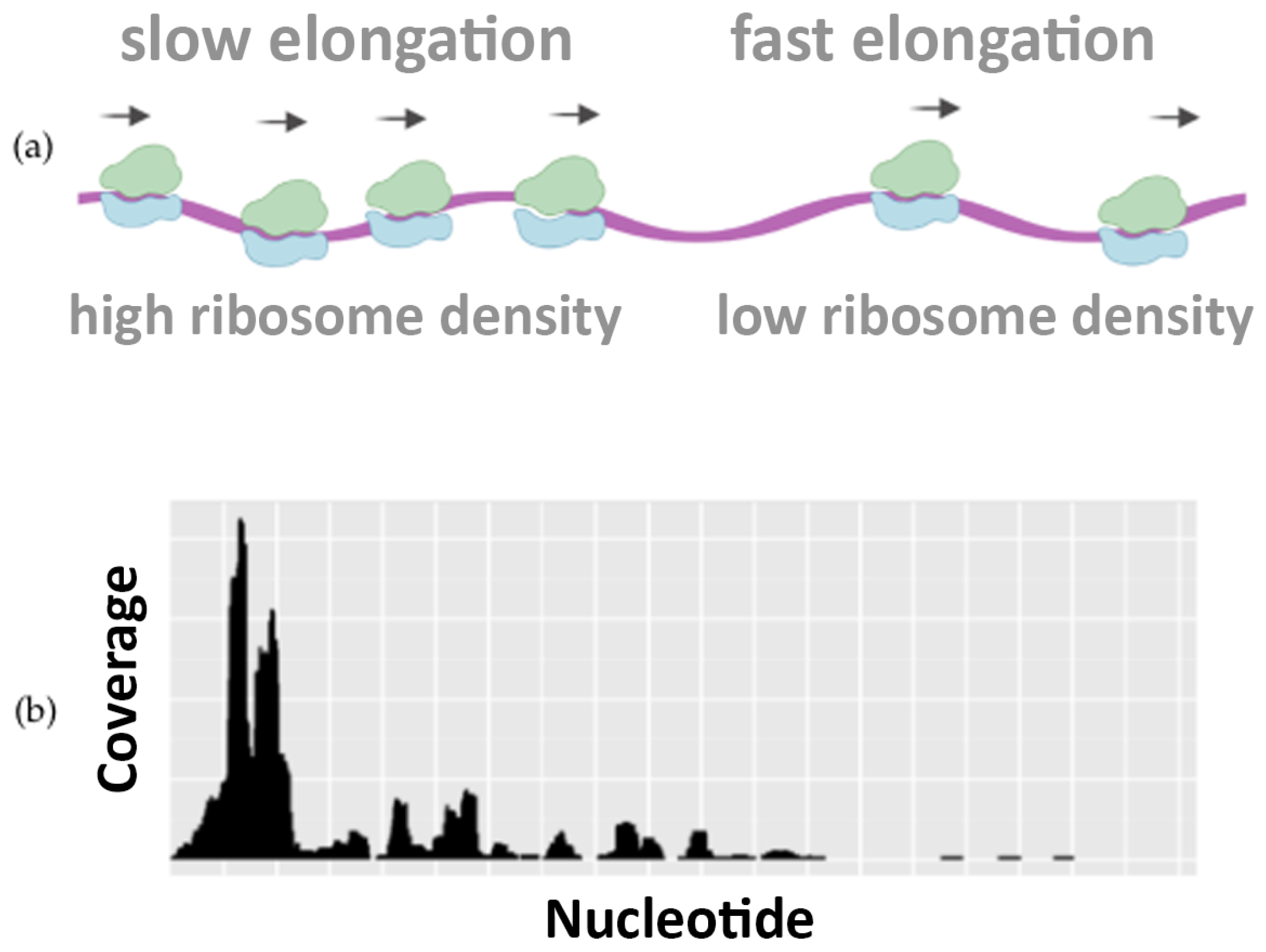
Interestingly, the nucleotide–level resolution of Ribo–seq experiments reveals the density of the ribosomes at each position along the mRNA template. Local differences in the density of Ribosome Protected Fragments (RPFs) along the Open Reading Frame (ORF) reflect differences in the speed of translation and elongation, determining regions where the translation is slower or faster.

Figure 1 illustrates how the translation speed is not uniform, highlighting the differences in ribosome occupancy. This piece of information is well visible in Ribo–seq profiling data and can be used to infer how the codon usage, the protein sequences, and other features can regulate the speed of translation [4].

Unfortunately, the reproducibility of Ribo–seq experiments can be affected by multiple variables due to the complexity of the experimental protocol and the lack of standardization in computational data analysis [5].

Thereofore, our work aims to overcome the aforementioned limitations by introducing a new statistical approach, designed to extract a set of highly reproducible profiles.

In particular, inspired by the seminal work proposed in [6], we perform a novel analysis procedure for Ribo–seq data that allows to identify the reproducible Ribo–seq profiles emerging from the comparison of independent Ribo–seq experiments performed in different laboratories under the same conditions. These significantly reproducible profiles are then collected into a library of consensus sequences, in which sub-regions characterized by different translation speeds can be isolated. The aforementioned procedure has been applied to E. coli sequences (Escherichia Coli (E. coli) is a bacterium that lives in the lower intestine of warm-blooded animals and has a genome composed by approximately 4,600,000 base pairs. E. coli contains a total of 4288 genes, with coding sequences which are long, on average, 950 base pairs and separated, on average, from 118 bases. Considering the protein counterpart, in E. coli, the average length of a coding region is 316.8 codons, whereas less than 1.8% of the genes are shorter than 60 codons.), resulting in 40 highly reproducible profiles.

Differently from [6], based on the collected data, a statistical analysis has been carried out that gave new insights on the dynamics of the ribosome translation, showing a statistically significant difference in the nucleotide composition between sub-sequences characterized by different translation speeds. Moreover, to validate the procedure, the selected highly reproducible profiles have been analyzed through state-of-the-art Machine Learning (ML) models, accurately classifying subsequences according to their speed of translation (slow or fast).We have made our source code public available (https://github.com/pandrein/Ribo-Seq-analysis, accessed on 29 June 2022). Furthermore, these experiments allowed to discover that the translation speed is modulated both by the nucleotide composition of the sequences and by the order in which they appear within each sequence.

The rest of the paper is organized as follows: Section 2 collects works from the literature dealing with related topics; Section 3 describes the ribosome profiling data extraction and preprocessing, together with their analyses based on both statistical and ML methods; Section 4 summarizes the results, discussing their meaning and their biological interpretation. Finally, Section 5 draws some conclusions and derives future perspectives.

2. Related works

The Ribosome profiling approach offers a promising method for developing unbiased translation models from data, but the quantitative analysis of ribosome profiling data is challenging, because of high measurement variance and the inability to distinguish the ribosome rate of translation. The Ribosome profiling strategy based on deep sequencing of ribosome–protected mRNA fragments enables genome–wide investigation of translation at the codon and sub–codon resolution [7].

In recent years, techniques based on machine learning have been employed with increasing frequency and intensity in many different fields, ranging from computer vision [8,9,10,11] to natural language processing [12,13,14] and bioinformatics [15,16]. The popularity of these approaches stems from their success in the automatic inference of complex functions directly from the data. In particular, both statistical and ML approaches have been successfully applied to non–biological sequential data classification tasks [17,18,19], in which each sequence is associated with a class label and the classification is performed on the whole sequence. Within bioinformatics, examples of ML applications include the prediction of splicing patterns and protein secondary structures, protein–protein interface prediction, protein subcellular localization, drug side-effect prediction, and DNA/RNA motif mining, to name just a few [20,21,22,23]. Moreover, ML and deep learning approaches have been used to process Ribo–seq data for gene annotation in prokaryotes [24], to predict ribosome stalling [25] and for micropeptide identification [26]. In particular, in [27], a deep learning based approach, called RiboMIMO, was proposed, based on a multi-input and multi–output framework, for modeling the ribosome density distributions of full-length mRNA Coding Sequence (CDS) regions. Through considering the underlying correlations in translation efficiency among neighboring and remote codons, and extracting hidden features from the input full-length coding sequence, RiboMIMO can accurately predict the ribosome density distributions along with the whole mRNA CDS regions, a problem strictly correlated with the one we intend to face in this paper. Indeed, we propose a machine learning-based approach to validate the extraction procedure of highly reproducible profiles, by classifying the translation speed of the extracted regions, which deeply depends on the ribosome density along mRNA.

3. Materials and Methods

In this work, a new software, written in Python, has been developed, which reproduces the procedure described in [6]. In this section, the method used to obtain a set of reproducible Ribo–seq profiles and their analysis through statistical and ML methods are presented. In particular, in Section 3.1, the procedure employed to extract the profiles is described, while in Section 3.3, a statistic analysis of the nucleotide composition is presented. Finally, in Section 3.4, two different ML approaches are proposed to analyze the data and asses their quality.

3.1. Ribosome Profiling Data Extraction

The Ribosomal profiling technique (Ribo–seq) is currently the most effective tool to study the protein synthesis process in vivo. The advantage of this method, over other approaches, lies in its ability to monitor translation by precisely mapping the position and number of ribosomes on an mRNA transcript. Ribo–seq involves the extraction of mRNA molecules associated with ribosomes undergoing active translation and a digestion phase, during which the RNase enzyme processes all the RNA molecules, with the exception of the “protected” parts, to which ribosomes are attached. This step is followed by rRNA depletion and preparation of the sequencing library as in an RNA–seq approach. However, since reads are obtained relating only to actively transcribed mRNA molecules, Ribo–seq better reflects the translation rate than mRNA abundance alone, although it requires particularly laborious preparation and is only applicable to species that have a reference genome available. The strategy employed in our work consists in the identification of high resolution Ribo–seq profiles through the systematic comparison of Ribo–seq datasets referring to experiments performed independently in different laboratories and in different time periods.

In particular, the approach is composed by the following phases:

• Preprocessing—the ORF–specific ribosome profiling data from multiple datasets are collected and then processed by a bioinformatic pipeline;
• Signal digitalization—Ribo–seq profiles are digitalized by associating to each nucleotide a slow or fast label;
• Comparison of digital profiles—Digital profiles are used to quantify similarities and differences between Ribo–seq profiles of different datasets referring to the same ORF.
• Identification of significantly reproducible Ribo–seq profiles—A set of highly reproducible profiles is obtained and, among them, reproducible sub-sequences are identified.

3.1.1. Preprocessing of Ribosome Profiling Data

To illustrate the statistical procedure employed in this work, we analyse a set of E. coli Ribo–seq profiles. For this purpose, the data stored in the Gene Expression Omnibus [28] repository were used. Specifically, our analysis concerns a systematic comparison of Ribo–seq profiles, each belonging to a different GEO series (A series is a collection of datasets that include at least one group of data—sample—from Ribo–seq experiments performed on E. coli in various conditions according to the most used experimental protocol.), referring to experiments performed culturing wild–type E. coli strains under control conditions. In particular, our analysis regarded a subset of eight samples (labelled from Dataset 1 to Dataset 8) obtained through experiments characterised by K–12 MG1655 genotype and cultured in a MOPS–based medium.

Table 1. The samples chosen for our analysis belong to different GEO series. Column 1: Dataset ID chosen to refer to the eight samples in this work; Column 2: GEO Series ID; Column 3: GEO Sample ID; Column 4: references. The listed ID can be used as access keys to the GEO Database (https://www.ncbi.nlm.nih.gov/geo/, accessed on 29 June 2022) to find a detailed description of both specific series and samples.

Dataset ID	GEO Series ID	GEO Sample ID	Ref
Dataset 1	GSE64488	GSM1572266	[29]
Dataset 2	GSE90056	GSM2396722	[30]
Dataset 3	GSE72899	GSM1874188	[31]
Dataset 4	GSE53767	GSM1300279	[32]
Dataset 5	GSE51052	GSM1399615	[33]
Dataset 6	GSE77617	GSM2055244	[34]
Dataset 7	GSE35641	GSM872393	[35]
Dataset 8	GSE88725	GSM2344796	[36]

reports the GEO Series ID and GEO sample ID of raw Ribo–seq dataset used in this experiment.

To reconstruct the Ribo–seq profiles starting from raw Ribo–seq data, represented by the FASTA format (The FASTA format is a text–based format for representing nucleotide sequences in which base pairs are indicated using single-letter codes [A,C,G,T] where A = Adenosine, C = Cytosine, G = Guanine, T = Thymidine), the reads are mapped against the whole set of coding sequences in E. coli, taken from the EnsemblBacteria database [37]. Then, we extracted and counted the number of reads mapping to each gene from the SAM alignment file (The Sequence Alignment Map (SAM) is a text–based format originally used for storing biological sequences aligned to a reference sequence.) using BEDTools [38]. The genomic coordinates are stored in a BED file (The BED file is a tab-delimited text file used to store genomic regions where each feature is described by chromosome, start, end, name, score, and strand.) to build the Ribo–seq profiles representing the input of the subsequent analysis. Each ORF can be associated to a specific Ribo–seq profile, a histogram that counts the number of reads that cover each nucleotide position. To realize the pairwise comparison of ORF–specific Ribo–seq profiles coming from independent datasets, we decided to proceed as described in the following.

3.1.2. Signal Digitalization Strategy

Firstly, we selected the ORFs in common between all the eight datasets highlighted in Table 1. For each ORF of each dataset, we generated a Ribo–seq profile. The Ribo–seq profiles (Figure 2, left side) are digitalized by comparing the profile heights at each nucleotide position (coverage) with its median value, computed along the entire ORF. We assign $+1$ to the positions having a coverage value higher than the median, $-1$ otherwise. The result is a digital Ribo–seq profile (Figure 2, right side) for each Ribo–seq profile, i.e., a vector having the length of the associated ORF and containing a sequence of $-1$ and $+1$.

3.1.3. Comparison of Digital Profiles

The digitalized profiles can be compared to detect matches, i.e., nucleotides characterized by an identical label ( Figure 2). Calculating the relative number of matches (the ratio between the number of matches and the length of the ORF) yields the matching score ($s_i{,}_k$). Intuitively, a matching score close to one could indicate a high degree of similarity between a pair of digitalized profiles, whereas a score around one-half could mean a very poor overlap because the observed matches are likely to have occurred by chance. Given each score has a certain probability of being obtained by chance, we decided to implement a statistical test able to assess the significance of the matching score [6].

For any Ribo–seq profile involved in a pairwise comparison, a large number of randomized profiles is generated by re-distributing the reads in random positions on the reference ORF. The randomized profiles are, in turn, compared pairwise yielding a large number of random matching scores that build each null distribution. Reiterating this process, we generated ${10}^4$ pairs of random Ribo–seq profiles and an equal number of digitalized random profiles that, compared pairwise, yielded ${10}^4$ random matching scores. These scores are used to build an ORF–specific null distribution which allows us to estimate the probability of obtaining each similarity score just by chance.

Given a pair of Ribo–seq profiles, the similarity score resulting from their comparison is tested for significance by comparing it to the corresponding ORF–specific null distribution. For each $s_{i,k}$ and the corresponding null distribution, we computed a z-score $z_{i,k}$, mapping each similarity score on a standard normal distribution.

Subsequently, we computed the p-values $p_{i,k}$, as the integral:

$$\begin{array}{c}\hfill p_{i,k}={\int }_{z_{i,k}}^{+\infty }{N}_S\left(z\right)dz\end{array}$$

where $N_S\left(z\right)$ is the standard normal distribution. Mapping the matching score on the null distribution will yield the p-value. The results of this process can be summarised into a matrix (called p-value matrix) containing all the computed p-values and composed by one column for each pairwise comparison and one row for each considered ORF (for a total of 3588 rows and 28 columns). For the sake of simplicity,

Table 2. Excerpt of the p-value matrix. Each column corresponds to a pairwise comparison between two datasets while each row contains the gene ID. For the sake of readability, only three columns and five rows are reported here.

	Dataset 1 vs. Dataset 2	Dataset 1 vs. Dataset 3	Dataset 1 vs. Dataset 4
alr	0.769298564	0.122368427	0.632263895
modB	0.165522551	0.056591384	0.601754757
cysZ	0.005770742	0.00011569	0.2021111
dfp	0.002343099	0.000384015	0.093624025
fruB	0.566785395	0.85548442	0.381131384

collects a small extract of such matrix. Each $p_{i,k}$ quantifies the probability of obtaining a similarity score at least as extreme as the corresponding $s_i{,}_k$, given that the null hypothesis is true. In our context, the lower the p-value, the lower the probability that the similarity between the compared pairs of (digitalized) Ribo–seq profiles occurs by chance. If the p-value will result below a given threshold, the compared Ribo–seq profiles will exhibit a significant degree of similarity.

3.1.4. Identification of Significantly Reproducible Ribo-seq Profiles

Our strategy consists in inspecting each row of the p-value matrix. We define reproducible the Ribo–seq profiles referring to those rows featuring all the p-values below a chosen significance threshold. To cast our strategy into a more rigorous statistical framework, we exploit the False Discovery Rate (FDR) concept and the Benjamini-Hockberg (BH) correction method for multiple tests. In this experiment, for any given row of the p-value matrix, we set an FDR threshold of 0.01. This means that we accept that 1% of profiles are reproducible by chance. Then, we counted how many p-values in each row resulted significant according to the BH method, and we defined reproducible those Ribo–seq profiles associated with the rows where 80% of the p-values are significant. Following this strategy, we found that, out of 3588 genes that are common to the eight datasets, 40 genes, listed in

Table 3. Genes with significantly reproducible Ribo–seq profiles across the eight datasets. Column 1: Gene ID. Column 2: Annotation.

Genes ID	Annotation
rodZ	Cytoskeleton protein RodZ
arcB	Aerobic respiration control sensor protein ArcB
dld	Quinone-dependent D-lactate dehydrogenase
dnaX	DNA polymerase III subunit tau
fhuA	Ferrichrome outer membrane transporter/phage receptor
glnA	Glutamine synthetase
gltB	Glutamate synthase NADPH large chain
hisS	Histidine-tRNA ligase
infB	Translation initiation factor IF-2
katG	Catalase-peroxidase
malF	Maltose transport system permease protein MalF
metG	Methionine-tRNA ligase
mukB	Chromosome partition protein MukB
ompC	Outer membrane protein C
parC	DNA topoisomerase 4 subunit A
secY	Protein translocase subunit SecY
purL	Phosphoribosylformylglycinamidine synthase
rne	Ribonuclease E
sucA	2-oxoglutarate dehydrogenase E1 component
tufA	Elongation factor Tu 1
tufB	Elongation factor Tu 2
leuA	2-isopropylmalate synthase
hokB	Toxin HokB; Toxic component of a type I toxin-antitoxin (TA) system.
acnA	Aconitate hydratase A
ubiJ	Ubiquinone biosynthesis protein UbiJ
lptD	LPS-assembly protein LptD
rpnC	Recombination-promoting nuclease RpnC
rpnA	Recombination-promoting nuclease RpnA
fdoG	Formate dehydrogenase-O major subunit
wbbH	O-antigen polymerase
wbbI	Beta-1,6-galactofuranosyltransferase WbbI
wbbK	Putative glycosyltransferase WbbK
rpnE	Inactive recombination-promoting nuclease-like protein RpnE
lpoA	Penicillin-binding protein activator LpoA
gspD	Putative type II secretion system protein D
yfjI	Uncharacterized protein YfjI; Phage or Prophage Related
rlmL	Ribosomal RNA large subunit methyltransferase K/L
rsxC	Electron transport complex subunit RsxC
yfcI	Recombination-promoting nuclease RpnB
gtrS	Uncharacterized protein YfdI; Putative ligase

, have a significantly reproducible Ribo–seq profile.

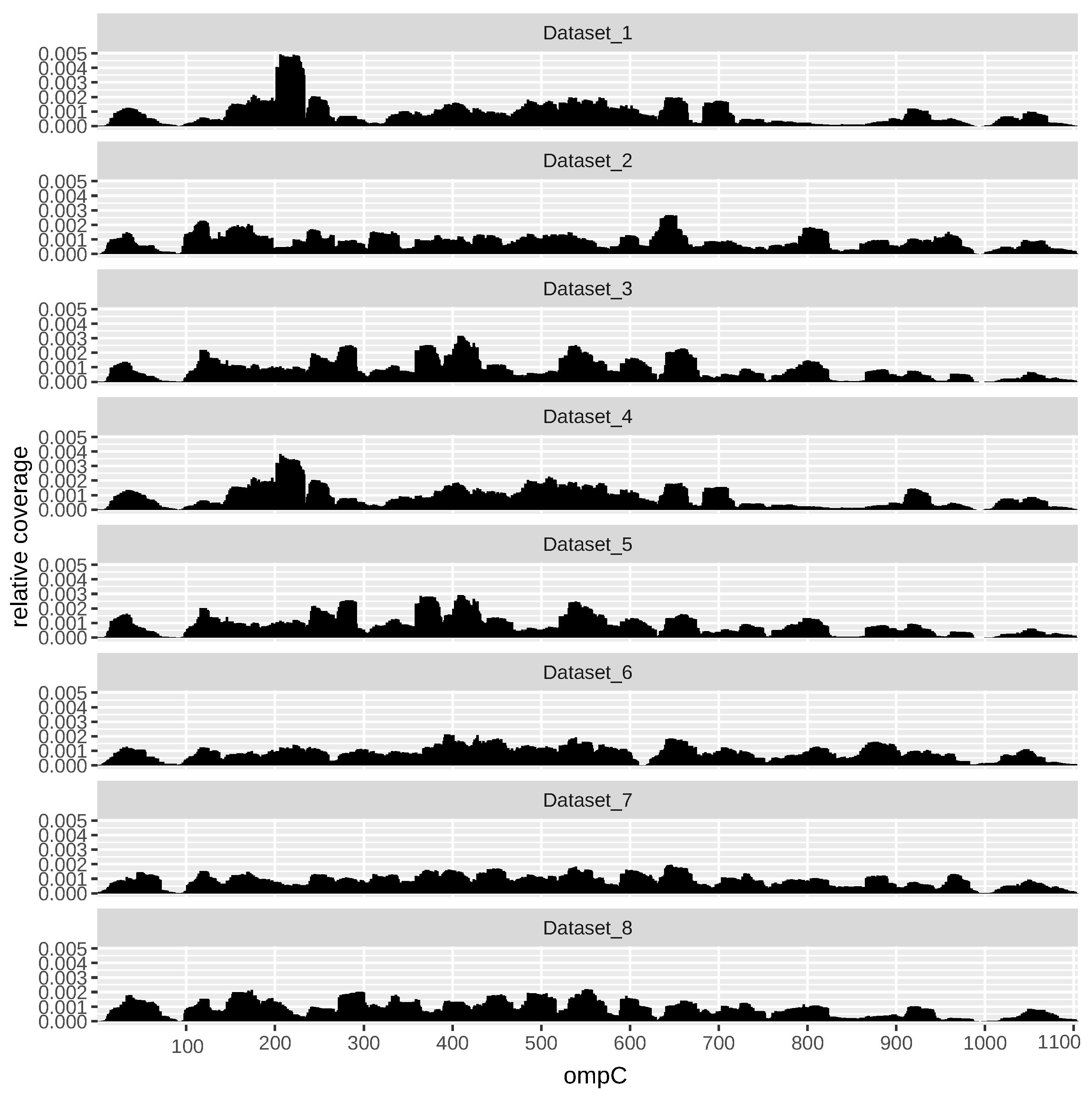
As an example, Figure 3 shows the profile across all datasets of the gene ompC (EG10670). OmpC, also known as outer membrane (OM) protein C, is a porin of gram-negative bacteria tightly associated with the peptidoglycan layer. It has been recognized to have a crucial role in the non-specific diffusion of small solutes such as sugars, ions and amino acids across the outer membrane of the cell [39].

To highlight which specific regions within the Ribo–seq profiles are similar to each other, we built a consensus sequence. The consensus sequence is a character string representing the nucleotides of the reference ORF and, in Figure 4, it is colored red in those positions where a peak is present in at least 80% of profiles (i.e., the digitalized profiles values are $+1$ and the ribosome proceeds slower), and green where a valley is located. The black color, instead, will be used in all other cases and the label assigned to these regions will be 0.

3.2. Dataset

The presented analysis has been applied to the prokaryotic organism E. coli on 3588 Ribo–seq profiles across eight independent datasets, revealing that only 40 profiles are significantly reproducible. The digitalization process described above produces a target belonging to $\{-1,+1,0\}$ for each nucleotide of the sequence. Based on the obtained profiles, a dataset (“SubsequencesDataset”) has been constructed, consisting in mRNA reproducible sub-sequences with a uniform target (since they are reproducible, the target is not 0). In particular, 459 sub-sequences of variable length have been obtained, of which 264 are characterized by a slow translation ($+1$) and 195 by a fast translation ($-1$). In order to obtain a fixed-length vector of 36 elements, padding have been applied to the extracted regions, consisting of nucleotides of the original consensus sequence. Each nucleotide has been encoded with a 1-hot vector of 4 elements, representing one of the four possible nucleotides. The “SubsequencesDataset” is further splitted in a training set of 413 sub-sequences and a test set of 46 sub-sequences. Moreover, a validation set was built, randomly selecting $15\%$ of the training set sub-sequences, to give an unbiased evaluation of the model performance during training, and for keeping overfitting under control. The splitting was done ensuring that sub-sequences in the test set and in the training set are taken from different genes. Each sub-sequence is associated with a target which corresponds to its translation speed.

3.3. Statististical Analysis on the Nucleotide Composition of the Subsequences

Inferential statistics can provide insights on the specific patterns and characteristics of the data and highlight relationships between variables. The “SubsequencesDataset”, obtained with the procedure described in Section 3.2, is analyzed to explore the nucleotide composition of the mRNA sub-sequences, relating to the assigned labels ($+1$ and $-1$).

First, the relative frequency of each nucleotide (A, T, G, C) has been computed. To assess the significance of our results and to find out whether the obtained frequencies are typical of a certain speed or the correspondence is just obtained by chance, we built a statistical test. The aim of the test is to assign a probability value (p-value) to the following null hypothesis: the slow and fast sub-sequences are characterized by a random nucleotide composition. In order to test this hypothesis, ${10}^4$ new profiles are generated by randomizing the nucleotide sequence, keeping fixed the $+1$ and $-1$ labels and therefore the length of the original sub-sequences. In each of the obtained sequence, the relative frequencies of the four nucleotides within the fast and slow sub-sequences can be calculated. This procedure leads to eight null distributions of relative frequencies, one for each nucleotide both for slow and fast translation. Comparing the null distributions against the original relative frequencies allows to calculate the p-values. In particular, if the original frequency is lower than the mean of the null distribution, we define the p-value as the probability of a random sub-sequence to show a relative frequency smaller than that observed in the original sub-sequence. On the contrary, if the original frequency is higher than the mean of the null distribution, the p-value is calculated as the probability of finding by chance a higher relative frequency value. If the p-value lies under the significance threshold of $0.05$, the null hypothesis of completely random nucleotide frequencies is rejected. This indicates a statistically significant difference in the nucleotide composition between slow/fast and randomly generated sub-sequences.

3.4. Data Validation with Neural Network Models

In this section, the informative content of the obtained data has been validated using a machine learning approach. This is achieved by employing common neural network architectures on the “SubsequencesDataset” (see Section 3.2) to predict the translation speed class: “slow” or “fast”. In our specific problem, exploiting a network architecture can reveal whether there is enough information in the data to classify the sub-sequences into slow and fast with high accuracy. To perform this task, we used two different types of data: vectors and sequences. In fact, we initially considered four-dimensional vectors that collect the relative frequencies of occurrence of the four nucleotides and then we considered the entire sequence, to evaluate whether the order in which the nucleotides are arranged helps to capture the translation rate signal. Consistently, the experiments were carried out by applying two different neural network architectures: Multilayer Perceptrons (MLPs) [40] and Convolutional Neural Networks (CNNs) [41]. While MLPs are good at processing vectors, indeed, CNNs are powerful machine learning models that can be used to directly process complex data, sequences in our case. Hence, we have first predicted the translation speed based only on the nucleotide composition of the sub-sequence while, in a second set of experiments, we employed a CNN to process each sub-sequence.

3.4.1. MLP Analysis Based on the Nucleotide Frequencies

The MLP input is a four-dimensional vector whose elements correspond to the relative frequency value of each nucleotide in the sequence (in the order (A, T, G, C), see Figure 5). The goal is to determine how much information is carried by this simple statistic, regardless of the order in which the nucleotides appear in the sequence. The MLP has a single hidden layer with four neurons and an output layer with two neurons. A Softmax function is applied on the output layer, which produces the probability estimated by the network for each class (slow or fast) [42]. The network has been trained with the Adam optimizer, with an initial learning rate of 0.05.

3.4.2. Convolutional Neural Network Analysis Based on Sub-Sequences

While the MLP architecture can only process vectorial data, CNNs can take full advantage of sequential information. The CNN multilayer design allows to extract a hierarchy of representations from the data while the implemented weight sharing guarantees to limit the number of parameters with respect to a fully connected architecture. In our experiments, the model input are the nucleotide sub-sequences collected in “SubsequencesDataset”. The CNN elaborates the input to produce a prediction about the translation speed associated with the sequence. Specifically, our CNN architecture comprises two successive 1-D convolutional layers, with average pooling employed between the layers, followed by two fully connected layers. The two-class probability distribution output of the network is produced by using a Softmax activation function on the output of the second fully-connected layer. The 1-D convolutional layers are based on 16 kernels with dimension three and a ReLU activation function, applied to each layer [43]. The optimization of the network parameters is performed by the Adam optimizer using early stopping [44]. The overall network architecture is described in Figure 6.

3.4.3. Ensemble Convolutional Neural Networks

In the last experiment, an ensemble [45] of seven CNNs has been employed to produce a more stable and accurate prediction. Each CNN receives as input the nucleotide sub-sequences contained in the “SubsequencesDataset”. The seven CNNs have been trained independently. In the test phase, their output has been averaged to produce the final result. More specifically, the Softmax CNN output for each class (slow and fast) is averaged among the seven networks that compose the ensemble.

4. Results and Discussion

In the following, we report the results of the experimental analysis described above. In particular, in Section 4.1, the outcome of the statistical analysis on the frequency of nucleotides is presented while, in Section 4.2, the results of the machine learning analysis is outlined.

4.1. Statistical Analysis on the Nucleotide Frequencies

The first step of the statistical analysis consists in computing the relative frequencies of each nucleotide in the fast and slow sub-sequences, respectively. As it can be observed in

Table 4. Relative nucleotide frequency across fast sub-sequences.

Nucleotide	Frequency
A	0.328
T	0.257
G	0.216
C	0.209

, showing the nucleotide frequencies in the fast sub-sequences, adenine has a concentration which is significantly larger than those of the other nucleotides. In particular, adenine shows a relative frequency of approximately 0.32, while cytosine has the lowest frequency (0.2). Instead,

Table 5. Relative nucleotide frequency across slow sub-sequences.

Nucleotide	Frequency
A	0.240
T	0.228
G	0.274
C	0.258

reports the frequency values in slow sub-sequences. In the latter case, both guanine and cytosine have the highest relative nucleotide frequencies (0.27 and 0.26, respectively).

To assess the significance of the results, the statistical test described in Section 3.3 has been performed. The purpose of the test is to determine whether the frequencies obtained are specific characteristics of fast and slow sub-sequences or they are simply a product of chance. Actually, the results show a p-value equal to zero for every nucleotide, for both fast and slow sub-sequences. In our context, the lower the p-value, the lower the probability that the nucleotide frequencies for the two classes occur by chance. The obtained results suggest that the relative frequencies of the four nucleotides are significantly different from those occurring randomly. In particular, we can observe that nucleotides A and T have a higher frequency in fast sequences than G and C. Instead, the frequency of nucleotides G and C is significantly higher in slow sequences than those of A and T. Based on this evidence, the proposed method for the identification of reproducible Ribo–Seq profiles was able to correctly detect sub-sequences characterized by a higher information content with respect to random sub-sequences, confirming the validity of our new approach.

Moreover, some insights are provided by Figure 7, which reports the distribution of the sub-sequences across the whole dataset, based on their nucleotide composition. In particular, each dot on the plane represents a sequence, characterized by the relative frequencies of pairs of nucleotides. The color represents the translation speed: orange and blue dots correspond to slow and fast sub-sequences, respectively. Interestingly, it can be observed that selecting the pairs of nucleotides A–T and G–C, the fast and slow sub-sequences identify two clusters located in distinct regions of the plane.

4.2. Performance of the Neural Network Models

4.2.1. MLP Classification Based on Nucleotide Frequencies

In this experiment, a Multi-Layer Perceptron is used to predict the translation speed of sequences based only on their nucleotide composition. The model performance is summarized across five runs and reported in

Table 6. Summary of the results obtained with the MLP model. We collect the obtained test set metrics computed over five different runs. The last two rows report the average over the runs and the corresponding standard deviation.

MLP
Run	Precision	Recall	F1-Score	Accuracy
1	70.83	89.47	79.07	81.63
2	70.80	89.51	79.06	80.62
3	72.00	94.74	81.82	83.67
4	66.67	94.74	78.26	79.59
5	75.00	94.74	83.72	85.71
Average	71.06	92.64	80.39	82.24
Standard Dev.	2.68	2.57	2.06	2.20

. It can be noted that the network reaches on average 82.24% accuracy over the test set, while the standard deviation between different runs is 2.20%. In fact, these results are surprising, given that the only information used by the model is the nucleotide composition of the sub-sequences. Moreover, the results are compared with those obtained by training the MLP on random sub-sequences, in order to demonstrate that the reproducible sub-sequences are significantly more informative. Indeed, as reported in Table 6, the performance obtained on reproducible sub-sequences is significantly higher than that obtained on random sub-sequences, validating the significance of our approach.

4.2.2. CNN Classification Based on the Entire Sequence

The model performance is summarized across five runs in

Table 7. Summary of the results obtained with the 1-D CNN model. We collect the test set metrics computed over five different runs. The last two rows report the average over the runs and the corresponding standard deviation.

CNN
Run	Precision	Recall	F1-Score	Accuracy
1	96.00	90.00	93.00	91.84
2	96.00	87.00	91.00	89.80
3	93.00	90.00	92.00	89.80
4	100.00	77.00	87.00	85.71
5	93.00	90.00	92.00	89.80
Average	95.60	90.00	91.00	89.39
Standard Dev.	2.88	5.20	2.35	2.24

.

The achieved classification accuracy is 89.39%. It is worth noting that, by training a significantly more complex network than the MLP, and by providing a sequential data input, the accuracy increases by approximately eight percentage points. The obtained results clearly show that this model can extract useful information from a limited amount of data in a better way than MLPs, achieving a very high accuracy. Nonetheless, the standard deviation between the runs is 2.24%, which proves that the results are rather steady but still influenced by the parameter initialization. Therefore, to further improve performance, we have set up a more complex architecture consisting of seven CNNs: each of them provides a different prediction, i.e., a pair of probabilities describing the class membership of a sequence (slow or fast). The results of the experiments performed by the CNN ensemble are summarised in

Table 8. Summary of the results obtained with the CNN-ensemble model. We collect the obtained test set metrics computed over five different runs. The last two rows report the average over the runs and the corresponding standard deviation.

ENSEMBLE: 7 CNN
Run	Precision	Recall	F1-Score	Accuracy
1	96.00	90.00	93.00	91.84
2	96.00	87.00	91.00	89.80
3	96.00	90.00	93.00	91.84
4	96.00	90.00	93.00	91.84
5	93.00	90.00	92.00	89.80
Average	95.40	90.00	92.40	91.02
Standard Dev.	1.34	1.22	0.89	1.12

.

Our model reaches an accuracy of 91.02%, with a standard deviation of 1.12%. As expected, the accuracy of the ensemble CNN is improved while the variance is significantly decreased. Indeed, the ensemble model is very effective in the sub-sequence classification and also provides very stable results across different training runs.

5. Conclusions

In this paper, we have proposed an innovative method to characterize highly reproducibile Ribo–seq profiles. Ribo–seq data have been analysed through statistical analyses and state-of-the-art machine learning models, extremely effective in predicting the ribosome translation speed. In fact, using neural network architectures capable of processing both plain and sequential data, we have been able to obtain high accuracy, also proving that fundamental information is contained both in the nucleotide composition of the sequences and in the order in which nucleotides appear within each sequence. In this way, our work opens new exciting frontiers in the analysis of the ribosome translation dynamics in different organisms. Indeed, we have conducted a preliminary analysis of Ribo–seq profiles referring to liver tumours and their adjacent noncancerous normal liver tissues from ten patients with hepatocellular carcinoma (HCC) [46], achieving promising results. For what concerns the machine learning analysis, once we have obtained the consensus sequences, we carried on a preliminary study exploiting the same neural architectures employed on the E. coli datasets. Nonetheless, given the increased complexity of the human data, we believe that a further analysis is necessary, in particular defining ad-hoc neural architectures and with a specialized hyperparameter search, to improve performance. Finally, it is worth mentioning that our method represents an effective approach for any kind of Ribo–seq data, to investigate an extremely relevant open questions in biology, i.e., which features can influence the speed of the ribosome during translation.

References

1. Cao, R. mTOR signaling, translational control, and the circadian clock. Front. Genet. 2018, 9, 367. [Google Scholar] [CrossRef] [PubMed]
2. Ingolia, N.T.; Brar, G.A.; Rouskin, S.; McGeachy, A.M.; Weissman, J.S. The ribosome profiling strategy for monitoring translation in vivo by deep sequencing of ribosome-protected mRNA fragments. Nat. Protoc. 2012, 7, 1534–1550. [Google Scholar] [CrossRef] [PubMed]
3. Kuersten, S.; Radek, A.; Vogel, C.; Penalva, L.O. Translation regulation gets its ‘omics’ moment. Wiley Interdiscip. Rev. RNA 2013, 4, 617–630. [Google Scholar] [CrossRef] [PubMed] [Green Version]
4. Dana, A.; Tuller, T. Determinants of translation elongation speed and ribosomal profiling biases in mouse embryonic stem cells. PLoS Comput. Biol. 2012, 8, e1002755. [Google Scholar] [CrossRef] [PubMed] [Green Version]
5. Sin, C.; Chiarugi, D.; Valleriani, A. Quantitative assessment of ribosome drop-off in E. coli. Nucleic Acids Res. 2016, 44, 2528–2537. [Google Scholar] [CrossRef] [PubMed] [Green Version]
6. Valleriani, A.; Chiarugi, D. A workbench for the translational control of gene expression. bioRxiv 2020. [Google Scholar] [CrossRef] [Green Version]
7. Ingolia, N.T.; Ghaemmaghami, S.; Newman, J.R.; Weissman, J.S. Genome-wide analysis in vivo of translation with nucleotide resolution using ribosome profiling. Science 2009, 324, 218–223. [Google Scholar] [CrossRef] [PubMed] [Green Version]
8. Krizhevsky, A.; Sutskever, I.; Hinton, G.E. ImageNet Classification with Deep Convolutional Neural Networks. In Advances in Neural Information Processing Systems; Pereira, F., Burges, C., Bottou, L., Weinberger, K., Eds.; Curran Associates, Inc.: Red Hook, NY, USA, 2012; Volume 25. [Google Scholar]
9. He, K.; Zhang, X.; Ren, S.; Sun, J. Deep residual learning for image recognition. In Proceedings of the IEEE Conference on Computer Vision and Pattern Recognition, Las Vegas, NV, USA, 27–30 June 2016; pp. 770–778. [Google Scholar]
10. Andreini, P.; Ciano, G.; Bonechi, S.; Graziani, C.; Lachi, V.; Mecocci, A.; Sodi, A.; Scarselli, F.; Bianchini, M. A Two-Stage GAN for High-Resolution Retinal Image Generation and Segmentation. Electronics 2021, 11, 60. [Google Scholar] [CrossRef]
11. Esteva, A.; Kuprel, B.; Novoa, R.A.; Ko, J.; Swetter, S.M.; Blau, H.M.; Thrun, S. Dermatologist-level classification of skin cancer with deep neural networks. Nature 2017, 542, 115–118. [Google Scholar] [CrossRef] [PubMed]
12. Vaswani, A.; Shazeer, N.; Parmar, N.; Uszkoreit, J.; Jones, L.; Gomez, A.N.; Kaiser, Ł.; Polosukhin, I. Attention is all you need. In Proceedings of the Advances in Neural Information Processing Systems 30: Annual Conference on Neural Information Processing Systems 2017, Long Beach, CA, USA, 4–9 December 2017; Voume 30. [Google Scholar]
13. Devlin, J.; Chang, M.W.; Lee, K.; Toutanova, K. Bert: Pre-training of deep bidirectional transformers for language understanding. arXiv 2018, arXiv:1810.04805. [Google Scholar]
14. Brown, T.; Mann, B.; Ryder, N.; Subbiah, M.; Kaplan, J.D.; Dhariwal, P.; Neelakantan, A.; Shyam, P.; Sastry, G.; Askell, A.; et al. Language models are few-shot learners. Adv. Neural Inf. Process. Syst. 2020, 33, 1877–1901. [Google Scholar]
15. Andreini, P.; Bonechi, S.; Bianchini, M.; Geraci, F. MicroRNA signature for interpretable breast cancer classification with subtype clue. J. Comput. Math. Data Sci. 2022, 3, 100042. [Google Scholar] [CrossRef]
16. Ji, Y.; Zhou, Z.; Liu, H.; Davuluri, R.V. DNABERT: Pre-trained Bidirectional Encoder Representations from Transformers model for DNA-language in genome. Bioinformatics 2021, 37, 2112–2120. [Google Scholar] [CrossRef] [PubMed]
17. Ismail Fawaz, H.; Forestier, G.; Weber, J.; Idoumghar, L.; Muller, P.A. Deep learning for time series classification: A review. Data Min. Knowl. Discov. 2019, 33, 917–963. [Google Scholar] [CrossRef] [Green Version]
18. Wang, Z.; Yan, W.; Oates, T. Time series classification from scratch with deep neural networks: A strong baseline. In Proceedings of the IEEE 2017 International Joint conference on Neural Networks (IJCNN), Anchorage, AK, USA, 14–19 May 2017; pp. 1578–1585. [Google Scholar]
19. Zhao, B.; Lu, H.; Chen, S.; Liu, J.; Wu, D. Convolutional neural networks for time series classification. J. Syst. Eng. Electron. 2017, 28, 162–169. [Google Scholar] [CrossRef]
20. Jurtz, V.I.; Johansen, A.R.; Nielsen, M.; Almagro Armenteros, J.J.; Nielsen, H.; Sønderby, C.K.; Winther, O.; Sønderby, S.K. An introduction to deep learning on biological sequence data: Examples and solutions. Bioinformatics 2017, 33, 3685–3690. [Google Scholar] [CrossRef] [PubMed]
21. Pancino, N.; Rossi, A.; Ciano, G.; Giacomini, G.; Bonechi, S.; Andreini, P.; Scarselli, F.; Bianchini, M.; Bongini, P. Graph Neural Networks for the Prediction of Protein-Protein Interfaces. In Proceedings of the ESANN, Bruges, Belgium, 2–4 October 2020; pp. 127–132. [Google Scholar]
22. He, Y.; Shen, Z.; Zhang, Q.; Wang, S.; Huang, D.S. A survey on deep learning in DNA/RNA motif mining. Briefings Bioinform. 2021, 22, bbaa229. [Google Scholar] [CrossRef]
23. Klausen, M.S.; Jespersen, M.C.; Nielsen, H.; Jensen, K.K.; Jurtz, V.I.; Soenderby, C.K.; Sommer, M.O.A.; Winther, O.; Nielsen, M.; Petersen, B.; et al. NetSurfP-2.0: Improved prediction of protein structural features by integrated deep learning. Proteins Struct. Funct. Bioinform. 2019, 87, 520–527. [Google Scholar] [CrossRef] [PubMed] [Green Version]
24. Clauwaert, J.; Menschaert, G.; Waegeman, W. DeepRibo: A neural network for precise gene annotation of prokaryotes by combining ribosome profiling signal and binding site patterns. Nucleic Acids Res. 2019, 47, e36. [Google Scholar] [CrossRef] [PubMed] [Green Version]
25. Zhang, S.; Hu, H.; Zhou, J.; He, X.; Jiang, T.; Zeng, J. ROSE: A deep learning based framework for predicting ribosome stalling. bioRxiv 2016. [Google Scholar] [CrossRef]
26. Zhu, M.; Gribskov, M. MiPepid: MicroPeptide identification tool using machine learning. BMC Bioinform. 2019, 20, 559. [Google Scholar] [CrossRef] [PubMed] [Green Version]
27. Tian, T.; Li, S.; Lang, P.; Zhao, D.; Zeng, J. Full-length ribosome density prediction by a multi-input and multi-output model. PLoS Comput. Biol. 2021, 17, e1008842. [Google Scholar] [CrossRef] [PubMed]
28. Edgar, R.; Domrachev, M.; Lash, A.E. Gene Expression Omnibus: NCBI gene expression and hybridization array data repository. Nucleic Acids Res. 2002, 30, 207–210. [Google Scholar] [CrossRef] [PubMed] [Green Version]
29. Woolstenhulme, C.J.; Guydosh, N.R.; Green, R.; Buskirk, A.R. High-precision analysis of translational pausing by ribosome profiling in bacteria lacking EFP. Cell Rep. 2015, 11, 13–21. [Google Scholar] [CrossRef] [PubMed] [Green Version]
30. Morgan, G.J.; Burkhardt, D.H.; Kelly, J.W.; Powers, E.T. Translation efficiency is maintained at elevated temperature in Escherichia coli. J. Biol. Chem. 2018, 293, 777–793. [Google Scholar] [CrossRef] [Green Version]
31. Mohammad, F.; Woolstenhulme, C.J.; Green, R.; Buskirk, A.R. Clarifying the translational pausing landscape in bacteria by ribosome profiling. Cell Rep. 2016, 14, 686–694. [Google Scholar] [CrossRef] [PubMed] [Green Version]
32. Li, G.W.; Burkhardt, D.; Gross, C.; Weissman, J.S. Quantifying absolute protein synthesis rates reveals principles underlying allocation of cellular resources. Cell 2014, 157, 624–635. [Google Scholar] [CrossRef] [Green Version]
33. Subramaniam, A.R.; Zid, B.M.; O’Shea, E.K. An integrated approach reveals regulatory controls on bacterial translation elongation. Cell 2014, 159, 1200–1211. [Google Scholar] [CrossRef] [PubMed] [Green Version]
34. Burkhardt, D.H.; Rouskin, S.; Zhang, Y.; Li, G.W.; Weissman, J.S.; Gross, C.A. Operon mRNAs are organized into ORF-centric structures that predict translation efficiency. eLife 2017, 6, e22037. [Google Scholar] [CrossRef] [PubMed]
35. Li, G.W.; Oh, E.; Weissman, J.S. The anti-Shine–Dalgarno sequence drives translational pausing and codon choice in bacteria. Nature 2012, 484, 538–541. [Google Scholar] [CrossRef] [PubMed]
36. Baggett, N.E.; Zhang, Y.; Gross, C.A. Global analysis of translation termination in E. coli. PLoS Genet. 2017, 13, e1006676. [Google Scholar] [CrossRef]
37. Howe, K.L.; Contreras-Moreira, B.; De Silva, N.; Maslen, G.; Akanni, W.; Allen, J.; Alvarez-Jarreta, J.; Barba, M.; Bolser, D.M.; Cambell, L.; et al. Ensembl Genomes 2020—Enabling non-vertebrate genomic research. Nucleic Acids Res. 2020, 48, D689–D695. [Google Scholar] [CrossRef] [PubMed] [Green Version]
38. Quinlan, A.R.; Hall, I.M. BEDTools: A flexible suite of utilities for comparing genomic features. Bioinformatics 2010, 26, 841–842. [Google Scholar] [CrossRef] [PubMed] [Green Version]
39. Nikaido, H. Porins and specific diffusion channels in bacterial outer membranes. J. Biol. Chem. 1994, 269, 3905–3908. [Google Scholar] [CrossRef]
40. Murtagh, F. Multilayer perceptrons for classification and regression. Neurocomputing 1991, 2, 183–197. [Google Scholar] [CrossRef]
41. LeCun, Y.; Bengio, Y. Convolutional networks for images, speech, and time series. In The Handbook of Brain Theory and Neural Networks; MIT Press: Cambridge, MA, USA, 1995; Volume 3361, p. 1995. [Google Scholar]
42. Bridle, J.S. Probabilistic interpretation of feedforward classification network outputs, with relationships to statistical pattern recognition. In Neurocomputing; Springer: Berlin/Heidelberg, Germany, 1990; pp. 227–236. [Google Scholar]
43. Agarap, A.F. Deep learning using rectified linear units (relu). arXiv 2018, arXiv:1803.08375. [Google Scholar]
44. Kingma, D.P.; Ba, J. Adam: A method for stochastic optimization. arXiv 2014, arXiv:1412.6980. [Google Scholar]
45. Hansen, L.K.; Salamon, P. Neural network ensembles. IEEE Trans. Pattern Anal. Mach. Intell. 1990, 12, 993–1001. [Google Scholar] [CrossRef] [Green Version]
46. Zou, Q.; Xiao, Z.; Huang, R.; Wang, X.; Wang, X.; Zhao, H.; Yang, X. Survey of the translation shifts in hepatocellular carcinoma with ribosome profiling. Theranostics 2019, 9, 4141. [Google Scholar] [CrossRef]
Figure 1. Ribosome footprint density along the mRNA. The schematic distribution of translating ribosomes along the mRNA (a) and their ribosome profiles (b). Ribo–seq data show differences in the density of ribosomes: regions of fast elongation accumulate fewer ribosomes (low density) with respect to regions of slow elongation (high density).
Algorithms 15 00274 g001
Figure 2. Pairwise comparison of two Ribo–seq profiles of the ispB gene. Two independent Ribo–seq profiles (left) are obtained by computing the coverage at each nucleotide position within the ORF. x-axis: position within the ORF (nucleotides); y-axis (top): relative coverage (number of mapping reads/total number of reads) mapping on the ORF. The Ribo–seq profiles are compared to the median coverage to produce the digitalized ± 1 profiles (right). The digitalized profiles can be easily compared to detect matches (e.g., green rectangle) and mismatches (e.g., red rectangle). The ratio between the number of matches and the total number of nucleotides in the ORF gives the matching score. A score equal to one means a perfect match between the two profiles, whereas a score equal to one-half means a poor matching [6].
Algorithms 15 00274 g002
Figure 3. Example of a significantly reproducible Ribo–seq profile across the eight datasets (gene ompC, EG10670).
Algorithms 15 00274 g003
Figure 4. Part of a consensus sequence (computed for rsxC) indicating the nucleotides situated within fast (labelled with 1 ) and slow (labelled with + 1 ) translation regions. On nucleotides labelled with 0, no reproducible results have been obtained [6].
Algorithms 15 00274 g004
Figure 5. The MLP architecture having the nucleotide frequencies as input, and predicting the sequence class probability distribution (slow or fast).
Algorithms 15 00274 g005
Figure 6. The 1-D CNN exploited for sequence classification.
Algorithms 15 00274 g006
Figure 7. Representation of the sub-sequences on the plane based on the relative frequencies of two nucleotides. Each sub-sequence is represented by a dot on the plane. More specifically, the relative frequency of thymine and cytosine (a), adenine and thymine (b), cytosine and guanine (c), adenine and cytosine (d), thymine and guanine (e), and adenine and guanine (f), respectively, is shown. The colors represent the speed of translation: orange and blue dots indicate slow and fast sub-sequences, respectively.
Algorithms 15 00274 g007