Abstract
The adoption of deep neural networks for profiling side-channel attacks opened new perspectives for leakage detection. Recent publications showed that cryptographic implementations featuring different countermeasures could be broken without feature selection or trace preprocessing. This success comes with a high price: an extensive hyperparameter search to find optimal deep learning models. As deep learning models usually suffer from overfitting due to their high fitting capacity, it is crucial to avoid over-training regimes, which require a correct number of epochs. For that, early stopping is employed as an efficient regularization method that requires a consistent validation metric. Although guessing entropy is a highly informative metric for profiling side-channel attacks, it is time-consuming, especially if computed for all epochs during training, and the number of validation traces is significantly large. This paper shows that guessing entropy can be efficiently computed during training by reducing the number of validation traces without affecting the efficiency of early stopping decisions. Our solution significantly speeds up the process, impacting the performance of the hyperparameter search and overall profiling attack. Our fast guessing entropy calculation is up to 16× faster, resulting in more hyperparameter tuning experiments and allowing security evaluators to find more efficient deep learning models.
1. Introduction
Side-channel attacks (SCA) explore the unintentional leakages (power consumption, time, and electromagnetic emissions) from electronic devices running secret-sensitive operations such as embedded cryptographic algorithms. Profiling SCA, one of the most popular attack methods, is widely considered by developers and manufacturers when assessing worst-case security with the strongest adversary assumptions [1,2]. This attack assumes an adversary has a clone (open) device to build the strongest possible probabilistic model from collected side-channel measurements. Thus, the adversary applies the model to the victim’s devices to recover the secret. If the profiling model is correct and can learn existing side-channel leakages, a profiling attack phase usually requires fewer side-channel measurements compared to non-profiling attacks [3,4,5].
Template attacks are the most classic form of profiling SCA [1]. Template attacks theoretically represent the strongest profiling model because of the typical underlying statistical distribution of side-channel leakages following multivariate Gaussian (or normal) distributions. Machine learning methods have also been considered for profiling attacks [6,7], while their statistical parameters are learned from side-channel measurements rather than directly computed. Both Gaussian templates and machine learning models require feature selection. In the case of protected cryptographic implementations, the inability to make efficient feature selection (by selecting leakage samples with the highest Signal-to-Noise Ratio—SNR) may become a limiting factor to building optimal profiling models. Indeed, an effective feature selection requires a strong correlation between the leakages and processed intermediate data. For instance, in the presence of masking countermeasures, evaluators select the best features (or points of interest) by knowing the secret random masks. Then, one can deploy worst-case security evaluations to emulate the adversaries having access to the source code and secret shares during profiling. Additionally, template and machine learning-based models are susceptible to desynchronization effects in side-channel measurements, thus bringing additional challenges.
In recent years, the adoption of deep neural networks (DNNs) for profiling SCA has provided competitive (and, in some cases, superior) results compared to template attacks and classical machine learning-based methods, especially against AES implementations [8,9]. Without feature selection, which implies considering a weaker adversary, deep learning-based SCA can break cryptographic implementations protected with different countermeasures, such as Boolean masking and timing desynchronization [10]. Their high complexity follows the high learning capacity of DNNs; the expensive hyperparameter tuning becomes a limitation to fully exploring the full potential of deep learning (DL) to find vulnerabilities in software and hardware implementations.
To make the hyperparameter tuning process more efficient, one tries to define appropriate hyperparameter ranges, which directly reflect the number of trainable parameters. Indeed, smaller DNNs may limit the learning capacity of a model, underfitting the profiling side-channel traces and providing poor attack performance. On the other hand, adding too many network layers results in larger models that can easily overfit and learn a suboptimal profiling model, thus reducing the possibility of fitting the existing leakages. One straightforward way to avoid this problem is by allowing larger models to be trained with regularization, restricting the model’s capacity during training. Dropout, weight decay, and data augmentation are well-known methods for regularization, but their indirect influence on the attack performance adds newly introduced hyperparameters to the tuning process. Alternatively, early stopping is a very efficient regularization mechanism that monitors a validation metric and saves model parameters (weights and biases) when the training reaches the best generalization moment.
An efficient early stopping implementation in profiling SCA requires monitoring the most appropriate metric. Reducing cross-entropy loss has been widely considered as the main training objective [11]. This is especially advantageous when security evaluations follow worst-case assumptions where learning an optimal model, which has good generalization, should also provide the smallest possible validation loss value. Unfortunately, in profiling SCA, collected leakages are normally extremely noisy because of the environmental noise and implemented countermeasures. This usually leads the profiling process to end up in a suboptimal model. In those cases, as also empirically demonstrated in [12], validation loss and accuracy are inconsistent with SCA performance (i.e., key recovery) when the model is trained on protected datasets and, sometimes, overfits. Although the model can be optimized through gradient descent by minimizing the generic loss functions (such as categorical cross-entropy or negative log-likelihood), the calculation of guessing entropy (GE) from a set of validation traces is consistent and highly informative concerning the profiling model generalization in SCA. The main reason is that GE measures the summation likelihood for each possible key guess over a set of traces instead of assessing the individual probabilities of expected classes only, as is the case of machine learning metrics. Therefore, applying empirical GE as an early stopping metric tends to be reliable in assessing model generalization during training. However, empirical GE provides significant overheads depending on the validation set size. If early stopping is adopted with hyperparameter tuning, the process becomes very slow and, in some cases, impractical.
Contributions: To address the unsolved problem of having a highly efficient early stopping metric for profiling SCA, we propose a fast guessing entropy calculation by simply reducing the number of validation traces when accessing model generalization during training. By doing so, we show that the trained models do not suffer in performance, but the training process becomes significantly faster, allowing more detailed tuning. Our fast GE method (denoted FGE) is especially important when security evaluators relax adversaries’ assumptions and do not assume the knowledge of secret random masks. For this reason, deep learning-based profiling attacks tend to become more difficult, requiring a larger number of model search attempts. We compare the FGE method with state-of-the-art metrics for early stopping and guessing entropy in a deep learning-based SCA context. We show that FGE estimation is highly competitive and provides superior results with a negligible time overhead in all scenarios. With FGE, training with early stopping becomes faster, allowing hyperparameter tuning to deploy more search attempts and increasing the chances of selecting the model with higher performance. Our code is publicly available at https://github.com/AISyLab/fge_sca (accessed on 26 January 2023).
2. Background
In this section, we start by providing details about deep learning-based SCA and commonly used metrics. Afterward, we discuss the datasets we use in our experiments.
2.1. Deep Learning-Based SCA
Profiling SCAs consider the strongest adversary with access to a clone device running the target cryptographic algorithm. The adversary can query the clone device with any set of plaintext and chosen keys , and measure side-channel traces . These traces () are used for training the classification algorithm (i.e., to build a machine learning model). This phase is known as the training or profiling phase. During this phase, a validation set, , containing V traces, is selected from the profiling set to validate the model. Next, the adversary obtains measurements from the target device, where traces () are also captured with a known input but unknown (secret) key. The previously trained model is then exploited to recover the secret key used in the target device. This phase is known as the attack or test phase.
The template attack is the first introduced profiling approach in SCA [1]. This attack is also the best possible if sufficient (infinite) training traces are available [13]. Over the years, machine learning and deep learning algorithms have been shown to be more powerful in realistic scenarios, where noise and countermeasures further reduce the measurement quality [8,9]. While the profiling attack assumes a more powerful attacker than a non-profiling one, it requires significantly fewer traces than direct attacks to break the target: sometimes, only one trace could be sufficient.
Profiling SCA considers different methods to build or learn the statistical parameters representing a profiling model . The template attack assumes that side-channel leakages follow a multivariate Gaussian distribution [1]. The profiling phase consists of computing statistical parameters for a Gaussian mixture model ( is given by mean and covariance parameters). Thus, the model is built for each possible hypothetical leakage class (e.g., all possible Hamming weight values of a byte). In the attack phase, the adversary computes the probability that a new side-channel measurement (under attack) belongs to a specific class by using the computed probability density function from the approximate statistics.
In the case of machine learning (including deep learning), the statistical parameters (e.g., weights and biases in the case of neural networks) are learned from profiling traces during the training phase. The deep neural network can skip feature selection from , which is an advantage over classic machine learning techniques and template attacks [14].
In the attack phase, the adversary obtains a probability that the set of attack traces process the key byte , according to:
where is the leakage function computed from public information and the key hypothesis k. In our case, as we attack AES implementations running encryption executions, the leakage function is given by for the Identity leakage model or for the Hamming weight (HW) leakage model. The public value is the corresponding plaintext byte. The recovered (guessed) key byte k from is then obtained as:
If the model is good (i.e., it learned the leakage), then the recovered key is or at least is among the best guesses.
2.2. Metrics
The training process has the minimization of the selected loss function as the main goal. In this paper, we consider the categorical cross-entropy (CCE) as the loss function. As demonstrated in [12], due to the imbalanced dataset problem, the validation loss function values (including CCE) can be inconsistent with SCA metrics, which is also the case of SCA-based loss functions, as already proposed in [15,16]. Therefore, we must select a more efficient validation metric to assess the model’s performance for SCA.
Metrics such as guessing entropy are commonly used by an adversary to estimate the required effort to obtain the key [17]. A side-channel attack outputs a key guessing vector in decreasing order of probability, i.e., represents the most likely key candidate and the least likely key candidate. Guessing entropy is the average position of in . Commonly, the averaged value is calculated over multiple independent experiments to obtain statistically significant results. In this paper, this GE method is called empirical GE, and it is evaluated on a set of V validation traces, where the results of multiple key rank executions are averaged and performed on a partition Q from V.
2.3. Datasets
We consider three datasets commonly used in research on deep learning-based SCA.
2.3.1. ASCAD
We evaluate ASCAD datasets (https://github.com/ANSSI-FR/ASCAD, accessed on 26 January 2023) that contain side-channel measurements collected from the first-order protected software implementations of AES-128 running on an 8-bit AVR microcontroller [18]. There are two versions of the ASCAD dataset. The first version, ASCADf, has a fixed key and 60,000 traces. We split the dataset into 50,000, 5000, and 5000 for profiling, validation, and attack sets, respectively. The second version of the ASCAD dataset, ASCADr, has fixed and random keys, and it consists of 300,000 traces. In this case, we consider 200,000 for profiling (with random keys), 10,000 for validation, and 10,000 for the attack set. Both validation and attack sets have a fixed key. For both versions, we attack the third key byte (the first masked byte) by using the trimmed intervals already extracted and released by the authors of the dataset. Thus, we use a pre-selected window of 700 features for ASCADf, while for ASCADr, the window size equals 1400 features. For all experiments, the datasets are labeled according to the leakage model from the third S-box output byte in the first AES encryption round, i.e., and for the Identity and Hamming weight leakage models, respectively.
2.3.2. CHES CTF 2018
This AES dataset was released as part of the Capture-the-Flag (CTF) (https://chesctf.riscure.com/2018/content?show=training, accessed on 26 January 2023) competition in the Cryptographic Hardware and Embedded Systems (CHES) workshop in 2018. Four sets of 10,000 traces featuring encryption operations of a first-order masked software implementation were released for profiling purposes. These four sets were measured from four different STM32 platforms, namely A, B, C, and D. Two additional sets of 1000 traces were released as attack traces from devices C and D. In our experiments, we consider the three first sets A, B, and C, containing random keys and random inputs, as a set of 30,000 profiling traces. The set from device D, containing the fixed key, is then used as an attack and validation set. As side-channel measurements from CHES CTF contain 650,000 samples points per trace, we performed a window resampling on the traces and concatenated two intervals representing the mask processing before encryption and target intermediate operation, i.e., the S-Box in the first encryption round. The resulting dataset contains 4000 sample points. Both trace intervals are selected through a visual trace inspection. Note that source code and secret mask shares are not provided for this dataset.
2.4. Leakage Models
A leakage model is a function that maps the hypothetical data value toward the (approximation of) physical leakage of the device. Common leakage models take either the Hamming weight of the hypothetical data (assuming that the physical leakage is proportional to the number of ones in the intermediate value) or the direct value of the physical leakage (usually denoted as the identity leakage model).
3. Related Works
Optimizing performance in DL-based profiling SCA has received significant attention in recent years. Due to the expensive trial-and-error cost in the profiling phase, enhancing the performance in DL-based profiling SCA is challenging. In recent years, the SCA community has considered two main alternatives to improve the attack efficiency: (1) by defining small neural network models that are faster to train and easier to tune [8,9] and (2) by reducing the number of the required profiling traces during training [19]. Both solutions can have severe impacts on the attack or generalization performance. The first approach may result in models that underfit for more noisy leakages or leakages obtained from other devices (portability problem [20]). The second alternative speeds up the process; still, it may result in limited learnability due to the eventually low number of profiling traces. To obtain small neural network models, one needs to use appropriate techniques. Zaid et al. [8] and Wouters et al. [21] worked on designing methodologies for finding efficient neural network architectures. They both reported state-of-the-art results at the time while using significantly smaller neural networks than related works. Rijsdijk et al. [9] and Wu et al. [22] investigated advanced hyperparameter tuning techniques such as reinforcement learning and Bayesian optimization, respectively. The obtained results managed to further reduce the required number of attack traces to reach GE of 1, but with non-negligible computational complexity due to the tuning procedure. Perin et al. showed that even a random search could find very successful neural network models and that ensembles of neural networks can significantly outperform single models [23]. An alternative approach was followed by Perin et al., where the authors pruned neural networks while maintaining good performance [24]. The authors showed it was possible to remove up to 90% of the neurons and maintain the performance.
Besides the methods mentioned above, a third alternative uses efficient and reliable validation metrics to evaluate training and implement faster hyperparameter tuning (which can provide faster convergence) with larger models and larger profiling sets. Empirical GE (described in Section 2.1) can be very expensive to compute with larger validation sets, especially if used during training to detect the best training epoch. In a recent publication, Zhang et al. proposed a Guessing Entropy Estimation Algorithm (GEEA) to reduce the computational limitation cost of empirical GE for the full attacked key scenarios, which computes faster than empirical GE calculation on separate key bytes [15]. Indeed, empirical GE executes multiple key rank executions over multiple partitions of the dataset V, each containing Q measurements. GEEA, on the other hand, only requires one execution over the Q measurements.
Let us consider as a score indicating the probability that a measurement process key for a input (i.e., plaintext) . The GEEA first requires the calculation of pairwise subtractions of scores concerning the correct key, resulting in mean and variance for each key guess as follows:
where is the correct key. Then, the guessing entropy value is obtained as:
where is the cumulative density function of a normal Gaussian distribution .
Alternative solutions were proposed as new validation metrics for early stopping, stopping training sooner, and speeding up the process. In [25], the authors considered a mutual information (MI) approach between the output probabilities and validation labels to monitor the best epoch during training. The work of [26] monitors the epoch when the training achieves the minimal difference between the number of profiling and validation traces required to achieve a 90% success rate. The authors proposed a routine to abort training if this difference increases after reaching its minimum value. In our work, we also consider the mutual information metric for comparison. The method proposed in [26] is not considered in our comparative analysis as it is directly adapted to datasets with fixed keys in the profiling set, which is not the case of ASCADr. The method requires estimating the number of traces to reach a success rate of 90%, which implies obtaining the evolution of the success rate concerning the number of validation traces. This means that the success rate is computed Q times for each epoch, adding a significant time overhead to the process. Finally, Paguada et al. suggested an optimized early stopping algorithm that efficiently integrates the GE metric into the training phase [27].
As we can see, none of the mentioned approaches compute GE directly from the validation traces at the end of each training epoch. GEEA was proposed as a fast and more stable GE estimation, but it is not suggested to be used during network training. On the other hand, although GE can be a potential metric candidate, its computation could be very slow if more validation traces are considered (which is required for GE stability), finally providing significant overheads to the training process. Therefore, the SCA community did not consider directly applying GE (including GEEA) as the early stopping metric, especially in the hyperparameter search processes. This work provides a novel evaluation metric called fast guessing entropy and shows that significantly reducing the number of validation traces for GE estimation during training is reliable and efficient for early stopping, benefiting hyperparameter tuning optimization. Further information about deep learning-based side-channel analysis and challenges can be found in [28].
4. Fast GE for Early Stopping
Running a hyperparameter search without pre-selecting efficient ranges for each hyperparameter may fail to find powerful attack models. A solution could be searching for small models with restricted search ranges, as proposed in [8,21] or by setting the objective of the search as being a small model, as proposed by Rijsdijk et al. [9]. Small models are usually self-regularized, but they still suffer from a limited fitting capacity, which is particularly problematic for noisy and protected targets. An alternative is to allow larger models and add regularization to prevent overfitting [29]. Although regularization improves model generalization, regularized models with increased size require more training epochs, reducing the efficiency in a hyperparameter search process. As the number of training epochs is a critical hyperparameter to be determined, early stopping may become a standard approach.
To allow efficient early stopping with GE, we propose a fast GE calculation to reduce the empirical GE overheads. When used as an early stopping metric, FGE provides very small overheads to the training process, usually between 1.5% and 3.3%, while, e.g., empirical GE shows overheads between 18.59% and 28.19%, as reported in Section 5. Our idea consists in reducing the number of validation traces when computing GE for each processed epoch, which has multiple benefits in DL-based SCA. The pseudo-code showing how FGE is obtained is provided in Algorithm 1. As the algorithm shows, the main application of FGE is for the hyperparameter search process.
| Algorithm 1 Hyperparameter search with early stopping and fast guessing entropy. |
|
If the model converges, the attack is successful, and GE for a small number of validation traces can also indicate the best epoch to stop training efficiently. Using large validation sets for the metric calculation may obscure the real performance of the model: a model that overfits may also slowly decrease guessing entropy to 1 after processing enough validation traces. In contrast, FGE is more sensitive to the model’s performance change, thanks to its low usage of the validation traces. This situation is illustrated in Figure 1. As we can see in Figure 1a, with validation traces for empirical GE, the best epoch will be returned at the moment when GE is equal to 1. If the next epochs indicate a model that requires even fewer traces to succeed (which means better generalization), empirical GE will not capture that. On the other hand, using fewer traces allows us to obtain this convergence and recover the key with fewer attack traces, as shown in Figure 1b. Of course, the question here is: why would this be a problem if reaching a GE of 1 allows an adversary to recover the key? We can observe two main problems in this scenario. First, empirical GE with more traces provides more overhead and limits the number of hyperparameter search attempts, preventing us from finding a model that eventually breaks the target (which is the example of the model found in Figure 1). Second, from the current model, we would select trained parameters before it reaches its best attack performance or generalization capacity, which can also indicate overfitting on the validation set, possibly opening issues in portability scenarios (when the device used for profiling is different from the device used for attacks [20]). If a model generalizes, then GE will eventually decrease, and FGE should show this behavior too.
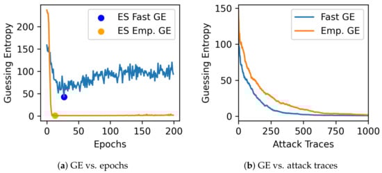
Figure 1.
Fast GE vs. empirical GE (ES = Early Stopping). In the left figure, we mark with a dot the epoch when GE is the lowest. Notice that FGE provides very similar results to empirical GE, making it an adequate choice for choosing when to stop the training process. In the right figure, we notice that FGE provides faster GE convergence, especially when the number of attack traces is limited.
5. Experimental Results
This section provides experimental results for (1) machine learning models obtained through a random search, (2) hyperparameter tuning for different validation metrics, and (3) state-of-the-art models and different validation metrics.
5.1. Hyperparameter Search Ranges
In this work, we only consider convolutional neural networks (CNNs) as they contain many hyperparameters to tune. Therefore, it becomes more challenging to find good hyperparameter combinations than, e.g., multilayer perceptrons. Consequently, the tuning of CNNs benefits more from an efficient evaluation strategy than tuning some simpler neural network architectures. Moreover, CNNs demonstrated good performance even in the presence of various hiding and/or masking countermeasures, and numerous SCA works consider only them, see, e.g., [8,9,10,30].
Convolutional neural networks commonly consist of convolutional layers, pooling layers, and fully connected layers. The convolution layer computes the output of neurons connected to local regions in the input, each computing a dot product between their weights and a small region connected to the input volume. Pooling decreases the number of extracted features by performing a down-sampling operation along the spatial dimensions. Finally, the fully connected layer computes the hidden activations or the class scores.
Table 1 provides the selected ranges for the hyperparameter tuning processes. These selected ranges result in a search space containing possible combinations. As we can see, we allow CNNs to contain up to eight hidden layers, combining convolution and dense layers. A pooling layer always follows each convolution layer. As the ASCADf and ASCADr datasets contain 50,000 and 200,000 profiling traces, respectively, larger models would tend to overfit.

Table 1.
Hyperparameter search space for CNNs (c in convolution filters indicates the convolution layer index).
5.2. Random Hyperparameter Search with Different Validation Metrics
We compare different early stopping metrics in a random hyperparameter search process for the two ASCAD datasets and different leakage models. The results for the CHES CTF dataset are only provided for the Hamming weight leakage model. Each randomly selected CNN is trained for 200 epochs, and we save the trained weights at the end of each epoch. At the end of the training, each early stopping metric indicates the best training epoch, and we restore the trained weights from that epoch. Then, as the training is finished, we compute GE for the attack set containing a larger number of traces. Note that 200 epochs is a relatively small number for training epochs, and, as shown in this section, stopping the training after 200 epochs may also deliver good results for some cases.
Table 2 gives the number of validation traces V considered for each early stopping metric, while the partition Q is the number of the traces used to calculate each specific metric. For instance, GE is the average of multiple key rank executions over Q traces, randomly selected from a larger set V for each key rank execution. This way, we set V greater than Q so that sampling each data in Q preserves a certain randomness. By doing so, the obtained results would indicate a better generalization capacity of models. For mutual information, we apply V validation traces. FGE estimation considers only 50 traces for Q and 500 for V. We tested other values for Q and V, from 20 to 200 (with a step of 10 traces), and 50 was the minimum value for Q and V, which still preserves the best results for FGE. This range was selected to align with the usually required number of attack traces reported in related works. More precisely, state-of-the-art techniques commonly require between 100 and 200 attack traces to break the considered datasets. At the same time, by considering a less than 100 attack traces setting, we allow for further improvements in the results.
Table 2.
Number of validation traces for each early stopping method.
We execute 500 searches for each dataset, considering the Hamming weight and identity leakage models. Table 3 provides the average time overhead in percentage for each considered metric. As we can see, the FGE estimation provides a maximum of 3.35% overhead among the four considered scenarios. For the ASCADr dataset, the overhead is only 1.19% and 1.49%, which can be considered negligible for the training time compared with its counterparts. As expected, the empirical GE and GEEA methods provide the largest overheads, although GEEA is faster than empirical GE. The mutual information method provides the second-best results, which is related to the more straightforward calculation than guessing entropy.
Table 3.
Average time overhead of different early stopping methods.
Table 4 provides the % that each metric can select a generalizing model with early stopping (model that reaches GE = 1 in the attack phase, which is indicated by line 13 in Algorithm 1) from the random search. Together with GEEA, the fast GE is a highly efficient metric (top two performance in all considered scenarios). Most importantly, we verified that FGE is always superior to the situation where no early stopping is used (200 epochs in the table) and with negligible overhead. For the case of the identity leakage models, FGE shows the best results.
Table 4.
Percentage of times a generalizing DNN was selected from each metric and from the training with all 200 epochs.
Figure 2 shows the results for the ASCADf dataset. When side-channel traces are labeled according to the Hamming weight leakage model, the correct key is recovered with 514 traces for the GEEA metric and 534 traces (the second best) with FGE early stopping metric. In the case of the identity leakage model, the best results are achieved for the FGE metric, where 101 attack traces are needed to achieve a GE equal to 1, which is aligned with state-of-the-art results [8,9,21]. The good performing results from the mutual information metric and the GE obtained with 200 epochs indicate the effectiveness of early stopping metrics in preventing the best model from overfitting. Again, we confirm that FGE is highly competitive in both leakage models and requires 10× fewer validation traces.
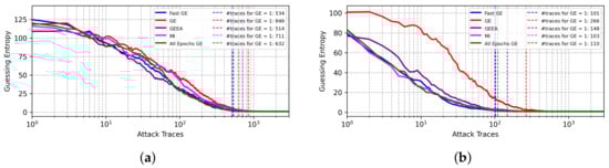
Figure 2.
GE results from best models selected from different early stopping metrics for the ASCADf dataset. (a) Hamming weight leakage model. (b) Identity leakage model.
For the ASCADr dataset, the results for FGE are also very promising, as shown in Figure 3. For the Hamming weight leakage model, FGE provides the best results, followed by the mutual information metric. In the case of the identity leakage model, the best result is obtained with all 200 epochs, showing that this number of epochs is appropriate for this best model found through a random search. The best results are obtained with the FGE metric when early stopping is considered.
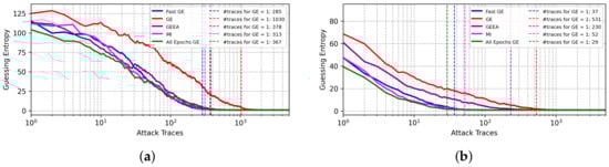
Figure 3.
GE results from best models selected from different early stopping metrics for the ASCADr dataset. (a) Hamming weight leakage model. (b) Identity leakage model.
Figure 4 provides results for the CHES CTF dataset. The FGE metric provides the second-best results after GEEA. The results for the CHES CTF dataset are only shown for the Hamming weight leakage model, as this dataset provides bad results with the identity leakage model, as discussed in [9].
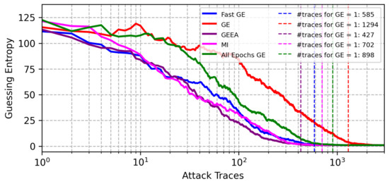
Figure 4.
GE results from best models selected from different early stopping metrics for the CHES CTF 2018 dataset (Hamming weight leakage model).
Furthermore, the performance of the best models selected from empirical GE as an early stopping metric provided less efficient results. As already mentioned in [15], empirical GE requires a very large validation set, and a more stable GE estimation can be obtained with the selection of larger validation sets. Of course, using larger validation sets provides an estimation of model generalization, and this is especially important for models that provide suboptimal performance and require more traces to show GE reduction for the correct key. However, computing GE for this large number of traces is undesirable as an early stopping metric due to significant time overhead.
5.3. Hyperparameter Tuning with Different Validation Metrics
This section analyzes how the evaluated early stopping metrics perform with Bayesian optimization (BO) for the hyperparameter search [22]. For that, we consider the open-source Bayesian Optimization method provided in the keras-tuner [31] Python package. We run Bayesian Optimization for 100 searches with ASCAD datasets and the Hamming weight and identity leakage models. We repeat each search process five times for each different early stopping metric. The guessing entropy results without early stopping (“all epochs” labels in the figures from the previous section) are omitted because keras-tuner inherently implements early stopping and, for this reason, it is not possible to select the best model by ignoring early stopping. The results reported in this section are extracted from the best-found model out of the five search attempts.
The results from BO for the ASCADf dataset are shown in Figure 5. The best results are obtained with FGE for both Hamming weight and Identity leakage models. In particular, for the Identity leakage model, as shown in Figure 5b, the best-found model achieves GE equal to 1 with less than half of the attack traces needed for GEEA. In these experiments, mutual information provides less efficient results.
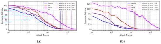
Figure 5.
GE results from best models found with BO with different early stopping metrics for the ASCADf dataset. (a) Hamming weight leakage model. (b) Identity leakage model.
Figure 6 provides BO results for the ASCADr dataset. For the Hamming leakage model, GEEA and FGE provide the best results. For the Identity leakage model, the results for FGE are superior, and only 60 attack traces are required for key byte recovery, while empirical GE requires 10× more attack traces to succeed. Again, the mutual information metric delivers the worst results.
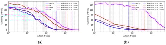
Figure 6.
GE results from best models found with BO with different early stopping metrics for the ASCADr dataset. (a) Hamming weight leakage model. (b) Identity leakage model.
Running hyperparameter tuning with Bayesian optimization for the CHES CTF dataset and the Hamming weight leakage model, the results obtained with FGE are significantly better than other validation metrics, as shown in Figure 7. We can see that FGE returns the best model that reaches GE equal to 1 in the attack phase with only 232 traces, while other metrics always require significantly more attack traces.
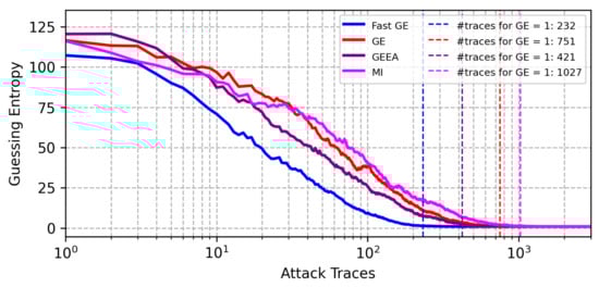
Figure 7.
GE results from best models found with BO with different early stopping metrics for the CHES CTF dataset (Hamming weight leakage model).
5.4. State-of-the-Art Models with Different Validation Metrics
The works of [8,9,21] proposed hyperparameter tuning for the ASCADf dataset and their models reported state-of-the-art results. In this section, we also verify whether FGE can improve the performance of those best models even more. This way, we provide attack results when applying early stopping to three CNN architectures. As the results for these CNN were reported for the Identity leakage model, we only consider that scenario in our analysis.
As shown in Figure 8, for the CNN models from [8,9], our FGE metric provides the best results. The results for the CNN model from [21] also put FGE among the best-performing metrics.
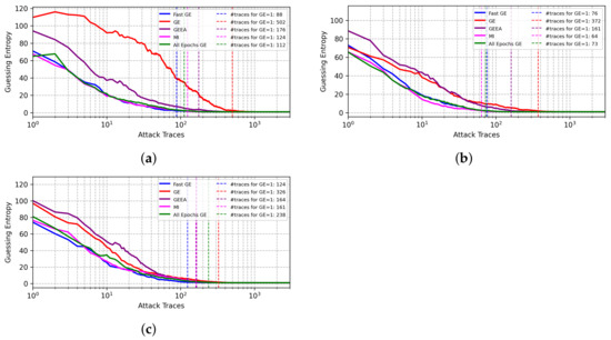
Figure 8.
Performance of different validation metrics on state-of-the-art CNN architectures, ASCADf dataset. (a) CNN from [8]. (b) CNN from [21].(c) Best CNN from [9].
6. Conclusions and Future Work
Profiling attacks are important during security evaluations because evaluators can determine if the device leaks information with high assurance. This is especially possible because assumptions during a profiling analysis consider that the target faces an adversary that can learn existing side-channel leakages in a supervised learning setting.
In a recent publication [32], Bronchain et al. showed through the lens of perceived information (PI) [33] how different profiling methods perform against protected cryptographic implementations. Their analysis allows security evaluators to conclude about the target’s leakages with the worst-case security. For that, the evaluator assumes that the adversary has knowledge of all intermediate secret shares during profiling and the source code. Consequently, such an evaluation provides conditions to implement optimal profiling models, where assumptions about the target (e.g., leakage model) contain as few errors as possible. Moreover, the evaluator can build a profiling model with sufficient traces, thus minimizing estimation errors.
The case of deep learning for profiling SCA brings a new perspective on profiling attacks. The main reason for that is related to the ability of a deep neural network to perform efficiently without feature selection. In practice, this means that the attacked interval contains several low SNR points of interest, and selecting the most leaky points of interest with a high SNR becomes more challenging. The advantages for security evaluations come from the fact that neural networks as profiling models can learn existing leakages even without feature selection and, in practice, deliver close to optimal results. The results for CNN architectures from Figure 8 are an example of this case. Of course, to reach an optimal deep learning profiling model, costly hyperparameter tuning needs to be implemented, especially for more protected targets.
Therefore, hyperparameter tuning must be as efficient as possible to reach optimal deep learning models without worst-case security assumptions. For that, assessing the model generalization during training becomes crucial, requiring fast and efficient validation metrics. We propose using a fast GE metric that requires significantly fewer validation traces in the GE calculation. Our results indicate that FGE as a validation metric delivers efficient and competitive early stopping results. Our technique is validated in different scenarios and shows good results with negligible time overheads. More precisely, FGE allows up to 16× faster guessing entropy calculation, resulting in more hyperparameter tuning experiments or fewer attack traces needed to reach a guessing entropy of 1. Thus, we consider FGE the method of choice for practical deep learning-based SCA hyperparameter tuning.
In future works, we will explore the efficiency of different validation metrics in portability settings and with different countermeasures in future work. Additionally, as this work contains results for convolutional neural networks only, it would be interesting to assess FGE performance with architectures such as multilayer perceptrons and residual neural networks.
Author Contributions
Conceptualization, G.P.; Methodology, S.P.; Software, G.P.; Validation, L.W. and S.P.; Investigation, G.P., L.W. and S.P.; Writing—original draft, G.P., L.W. and S.P. All authors have read and agreed to the published version of the manuscript.
Funding
This research received no external funding.
Institutional Review Board Statement
Not applicable.
Informed Consent Statement
Not applicable.
Data Availability Statement
The source code used for the experiments reported in this manuscript is available as a GitHub repository at https://github.com/AISyLab/fge_sca, accessed on 26 January 2023.
Conflicts of Interest
The authors declare no conflict of interest.
Abbreviations
The following abbreviations are used in this manuscript:
| SCA | Side-channel Attack |
| SNR | Signal-to-Noise Ratio |
| DNN | Deep Neural Network |
| AES | Advanced Encryption Standard |
| DL | Deep Learning |
| GE | Guessing Entropy |
| FGE | Fast Guessing Entropy |
| HW | Hamming Weight |
| CCE | Categorical Cross-Entropy |
| ASCAD | ANSSI SCA Database |
| ASCADf | ASCAD with a fixed key |
| ASCADr | ASCAD with random keys |
| CTF | Capture The Flag |
| CHES | Cryptographic Hardware and Embedded Systems |
| GEEA | Guessing Entropy Estimation Algorithm |
| MI | Mutual Information |
| CNN | Convolutional Neural Network |
| ReLU | Rectified Linear Unit |
| SELU | Scaled Exponential Linear Unit |
| ELU | Exponential Linear Unit |
| PI | Perceived Information |
| BO | Bayesian Optimization |
| ES | Early Stopping |
References
- Chari, S.; Rao, J.R.; Rohatgi, P. Template Attacks. In Proceedings of the Cryptographic Hardware and Embedded Systems—CHES 2002, Redwood Shores, CA, USA, 13–15 August 2002; Springer: Berlin/Heidelberg, Germany, 2003; pp. 13–28. [Google Scholar]
- Schindler, W.; Lemke, K.; Paar, C. A Stochastic Model for Differential Side Channel Cryptanalysis. In Proceedings of the Cryptographic Hardware and Embedded Systems—CHES 2005, 7th International Workshop, Edinburgh, UK, 29 August–1 September 2005; Rao, J.R., Sunar, B., Eds.; Lecture Notes in Computer Science. Springer: Berlin/Heidelberg, Germany, 2005; Volume 3659, pp. 30–46. [Google Scholar] [CrossRef]
- Kocher, P.C.; Jaffe, J.; Jun, B. Differential Power Analysis. In Proceedings of the Advances in Cryptology—CRYPTO ’99, 19th Annual International Cryptology Conference, Santa Barbara, CA, USA, 15–19 August 1999; Wiener, M.J., Ed.; Lecture Notes in Computer Science. Springer: Berlin/Heidelberg, Germany, 1999; Volume 1666, pp. 388–397. [Google Scholar] [CrossRef]
- Brier, E.; Clavier, C.; Olivier, F. Correlation Power Analysis with a Leakage Model. In Proceedings of the Cryptographic Hardware and Embedded Systems—CHES 2004: 6th International Workshop, Cambridge, MA, USA, 11–13 August 2004; Joye, M., Quisquater, J., Eds.; Lecture Notes in Computer Science. Springer: Berlin/Heidelberg, Germany, 2004; Volume 3156, pp. 16–29. [Google Scholar] [CrossRef]
- Gierlichs, B.; Batina, L.; Tuyls, P.; Preneel, B. Mutual Information Analysis. In Proceedings of the Cryptographic Hardware and Embedded Systems—CHES 2008, 10th International Workshop, Washington, DC, USA, 10–13 August 2008; Oswald, E., Rohatgi, P., Eds.; Lecture Notes in Computer Science. Springer: Berlin/Heidelberg, Germany, 2008; Volume 5154, pp. 426–442. [Google Scholar] [CrossRef]
- Banciu, V.; Oswald, E.; Whitnall, C. Reliable information extraction for single trace attacks. In Proceedings of the 2015 Design, Automation & Test in Europe Conference & Exhibition, DATE 2015, Grenoble, France, 9–13 March 2015; Nebel, W., Atienza, D., Eds.; ACM: New York, NY, USA, 2015; pp. 133–138. [Google Scholar]
- Lerman, L.; Bontempi, G.; Markowitch, O. A machine learning approach against a masked AES—Reaching the limit of side-channel attacks with a learning model. J. Cryptogr. Eng. 2015, 5, 123–139. [Google Scholar] [CrossRef]
- Zaid, G.; Bossuet, L.; Habrard, A.; Venelli, A. Methodology for Efficient CNN Architectures in Profiling Attacks. IACR Trans. Cryptogr. Hardw. Embed. Syst. 2020, 2020, 1–36. [Google Scholar] [CrossRef]
- Rijsdijk, J.; Wu, L.; Perin, G.; Picek, S. Reinforcement Learning for Hyperparameter Tuning in Deep Learning-based Side-channel Analysis. IACR Trans. Cryptogr. Hardw. Embed. Syst. 2021, 2021, 677–707. [Google Scholar] [CrossRef]
- Cagli, E.; Dumas, C.; Prouff, E. Convolutional Neural Networks with Data Augmentation Against Jitter-Based Countermeasures–Profiling Attacks Without Pre-processing. In Proceedings of the Cryptographic Hardware and Embedded Systems—CHES 2017—19th International Conference, Taipei, Taiwan, 25–28 September 2017; Fischer, W., Homma, N., Eds.; Lecture Notes in Computer Science. Springer: Berlin/Heidelberg, Germany, 2017; Volume 10529, pp. 45–68. [Google Scholar] [CrossRef]
- Masure, L.; Dumas, C.; Prouff, E. A Comprehensive Study of Deep Learning for Side-Channel Analysis. IACR Trans. Cryptogr. Hardw. Embed. Syst. 2020, 2020, 348–375. [Google Scholar] [CrossRef]
- Picek, S.; Heuser, A.; Jovic, A.; Bhasin, S.; Regazzoni, F. The Curse of Class Imbalance and Conflicting Metrics with Machine Learning for Side-channel Evaluations. IACR Trans. Cryptogr. Hardw. Embed. Syst. 2019, 2019, 209–237. [Google Scholar] [CrossRef]
- Lerman, L.; Poussier, R.; Bontempi, G.; Markowitch, O.; Standaert, F.X. Template Attacks vs. Machine Learning Revisited (and the Curse of Dimensionality in Side-Channel Analysis). In Lecture Notes in Computer Science; Springer: Cham, Switzerland, 2015; Volume 9064, pp. 20–33. [Google Scholar] [CrossRef]
- Lu, X.; Zhang, C.; Cao, P.; Gu, D.; Lu, H. Pay Attention to Raw Traces: A Deep Learning Architecture for End-to-End Profiling Attacks. IACR Trans. Cryptogr. Hardw. Embed. Syst. 2021, 2021, 235–274. [Google Scholar] [CrossRef]
- Zhang, J.; Zheng, M.; Nan, J.; Hu, H.; Yu, N. A Novel Evaluation Metric for Deep Learning-Based Side Channel Analysis and Its Extended Application to Imbalanced Data. IACR Trans. Cryptogr. Hardw. Embed. Syst. 2020, 2020, 73–96. [Google Scholar] [CrossRef]
- Zaid, G.; Bossuet, L.; Dassance, F.; Habrard, A.; Venelli, A. Ranking Loss: Maximizing the Success Rate in Deep Learning Side-Channel Analysis. IACR Trans. Cryptogr. Hardw. Embed. Syst. 2021, 2021, 25–55. [Google Scholar] [CrossRef]
- Standaert, F.X.; Malkin, T.G.; Yung, M. A unified framework for the analysis of side-channel key recovery attacks. Lect. Notes Comput. Sci. 2009, 5479, 443–461. [Google Scholar] [CrossRef]
- Benadjila, R.; Prouff, E.; Strullu, R.; Cagli, E.; Dumas, C. Deep learning for side-channel analysis and introduction to ASCAD database. J. Cryptogr. Eng. 2020, 10, 163–188. [Google Scholar] [CrossRef]
- Picek, S.; Heuser, A.; Perin, G.; Guilley, S. Profiled Side-Channel Analysis in the Efficient Attacker Framework. In Proceedings of the Smart Card Research and Advanced Applications: 20th International Conference, CARDIS 2021, Lübeck, Germany, 11–12 November 2021; Revised Selected Papers. Springer: Berlin/Heidelberg, Germany, 2021; pp. 44–63. [Google Scholar] [CrossRef]
- Bhasin, S.; Chattopadhyay, A.; Heuser, A.; Jap, D.; Picek, S.; Shrivastwa, R.R. Mind the Portability: A Warriors Guide through Realistic Profiled Side-channel Analysis. In Proceedings of the 27th NDSS, San Diego, CA, USA, 27 February–3 March 2020. [Google Scholar]
- Wouters, L.; Arribas, V.; Gierlichs, B.; Preneel, B. Revisiting a Methodology for Efficient CNN Architectures in Profiling Attacks. IACR Trans. Cryptogr. Hardw. Embed. Syst. 2020, 2020, 147–168. [Google Scholar] [CrossRef]
- Wu, L.; Perin, G.; Picek, S. I Choose You: Automated Hyperparameter Tuning for Deep Learning-based Side-channel Analysis. IEEE Trans. Emerg. Top. Comput. 2022, 1–12. [Google Scholar] [CrossRef]
- Perin, G.; Chmielewski, L.; Picek, S. Strength in Numbers: Improving Generalization with Ensembles in Machine Learning-based Profiled Side-channel Analysis. IACR Trans. Cryptogr. Hardw. Embed. Syst. 2020, 2020, 337–364. [Google Scholar] [CrossRef]
- Perin, G.; Wu, L.; Picek, S. Gambling for Success: The Lottery Ticket Hypothesis in Deep Learning-Based Side-Channel Analysis. In Artificial Intelligence for Cybersecurity; Stamp, M., Aaron Visaggio, C., Mercaldo, F., Di Troia, F., Eds.; Springer International Publishing: Cham, Switzerland, 2022; pp. 217–241. [Google Scholar] [CrossRef]
- Perin, G.; Buhan, I.; Picek, S. Learning When to Stop: A Mutual Information Approach to Prevent Overfitting in Profiled Side-Channel Analysis; Springer: Berlin/Heidelberg, Germany, 2021; Volume 12910, pp. 53–81. [Google Scholar] [CrossRef]
- Robissout, D.; Zaid, G.; Colombier, B.; Bossuet, L.; Habrard, A. Online Performance Evaluation of Deep Learning Networks for Profiled Side-Channel Analysis; Lecture Notes in Computer Science; Springer: Berlin/Heidelberg, Germany, 2020; Volume 12244, pp. 200–218. [Google Scholar] [CrossRef]
- Paguada, S.; Batina, L.; Buhan, I.; Armendariz, I. Being Patient and Persistent: Optimizing an Early Stopping Strategy for Deep Learning in Profiled Attacks. IEEE Trans. Comput. 2023, 1–12. [Google Scholar] [CrossRef]
- Picek, S.; Perin, G.; Mariot, L.; Wu, L.; Batina, L. SoK: Deep Learning-Based Physical Side-Channel Analysis. ACM Comput. Surv. 2023, 55, 227. [Google Scholar] [CrossRef]
- Srivastava, N.; Hinton, G.; Krizhevsky, A.; Sutskever, I.; Salakhutdinov, R. Dropout: A Simple Way to Prevent Neural Networks from Overfitting. J. Mach. Learn. Res. 2014, 15, 1929–1958. [Google Scholar]
- Kim, J.; Picek, S.; Heuser, A.; Bhasin, S.; Hanjalic, A. Make Some Noise. Unleashing the Power of Convolutional Neural Networks for Profiled Side-channel Analysis. Iacr Trans. Cryptogr. Hardw. Embed. Syst. 2019, 2019, 148–179. [Google Scholar] [CrossRef]
- O’Malley, T.; Bursztein, E.; Long, J.; Chollet, F.; Jin, H.; Invernizzi, L. KerasTuner. 2019. Available online: https://github.com/keras-team/keras-tuner (accessed on 26 January 2023).
- Bronchain, O.; Durvaux, F.; Masure, L.; Standaert, F.X. Efficient Profiled Side-Channel Analysis of Masked Implementations, Extended. IEEE Trans. Inf. Forensics Secur. 2022, 17, 574–584. [Google Scholar] [CrossRef]
- Bronchain, O.; Hendrickx, J.M.; Massart, C.; Olshevsky, A.; Standaert, F. Leakage Certification Revisited: Bounding Model Errors in Side-Channel Security Evaluations. In Proceedings of the Advances in Cryptology—CRYPTO 2019—39th Annual International Cryptology Conference, Santa Barbara, CA, USA, 18–22 August 2019; Proceedings, Part I. Boldyreva, A., Micciancio, D., Eds.; Lecture Notes in Computer Science. Springer: Berlin/Heidelberg, Germany, 2019; Volume 11692, pp. 713–737. [Google Scholar] [CrossRef]


Disclaimer/Publisher’s Note: The statements, opinions and data contained in all publications are solely those of the individual author(s) and contributor(s) and not of MDPI and/or the editor(s). MDPI and/or the editor(s) disclaim responsibility for any injury to people or property resulting from any ideas, methods, instructions or products referred to in the content. |
© 2023 by the authors. Licensee MDPI, Basel, Switzerland. This article is an open access article distributed under the terms and conditions of the Creative Commons Attribution (CC BY) license (https://creativecommons.org/licenses/by/4.0/).