Abstract
This paper introduces methods for parallelizing the algorithm to enhance the efficiency of event recovery in Spin Physics Detector (SPD) experiments at the Nuclotron-based Ion Collider Facility (NICA). The problem of eliminating false tracks during the particle trajectory detection process remains a crucial challenge in overcoming performance bottlenecks in processing collider data generated in high volumes and at a fast pace. In this paper, we propose and show fast parallel false track elimination methods based on the introduced criterion of a clustering-based thresholding approach with a chi-squared quality-of-fit metric. The proposed strategy achieves a good trade-off between the effectiveness of track reconstruction and the pace of execution on today’s advanced multicore computers. To facilitate this, a quality benchmark for reconstruction is established, using the root mean square (rms) error of spiral and polynomial fitting for the datasets identified as the subsequent track candidate by the neural network. Choosing the right benchmark enables us to maintain the recall and precision indicators of the neural network track recognition performance at a level that is satisfactory to physicists, even though these metrics will inevitably decline as the data noise increases. Moreover, it has been possible to improve the processing speed of the complete program pipeline by 6 times through parallelization of the algorithm, achieving a rate of 2000 events per second, even when handling extremely noisy input data.
1. Introduction
The SPD NICA experiment aims to investigate the characteristics of dense matter in extreme conditions in the field of high-energy physics. To achieve this, the SPD collaboration proposes the installation of a universal detector in the second interaction point of the NICA collider, which enables the study of the spin structure of the proton and deuteron using polarized beams [1].
The results of the SPD experiment are expected to provide significant contributions to our understanding of the gluon content of nucleons and to complement similar studies at RHIC, EIC at BNL, and the fixed-target facilities at LHC at CERN. It is crucial to conduct simultaneous measurements using different processes within the same experimental setup to minimize possible systematic errors.
Moreover, the experiment has the potential to investigate polarized and unpolarized physics during the first stage of NICA’s operation, with reduced luminosity and collision energy of the proton and ion beams.
As indicated in [1] and shown in Figure 1, the tracking part of the SPD setup includes the silicon vertex detector (SVD) and straw tube-based tracking (ST) system, which together consist of 53 measuring stations.
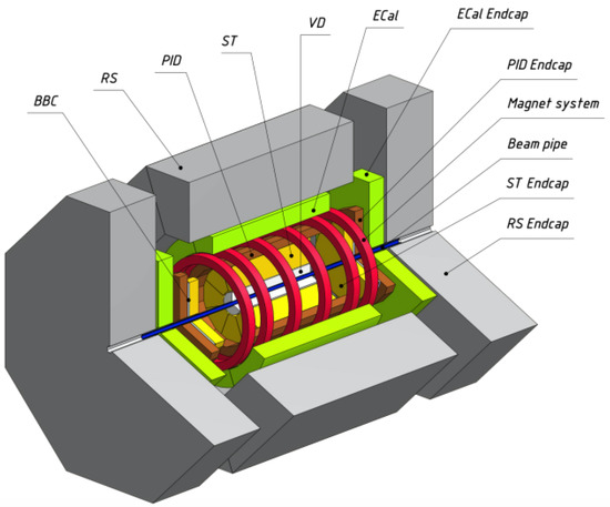
Figure 1.
General layout of the SPD setup [1].
Our focus is on the reconstruction of track measurements made in the SVD and ST systems. Unfortunately, both these detector systems have one significant disadvantage, caused by the data acquisition hardware itself. For instance, the straw tubes of every station are arranged in parallel in two layers, so that one of the coordinates of the passing track is read by the tubes of one layer and the other one by the other layer. When the number of passing tracks is more than one, this inevitably leads to the appearance of a large number of false readings—fake hits—in addition to the real ones.
Recognition of the trajectories of particles involved in collisions, for all high-energy experiments, is the main stage in the reconstruction of events, necessary to assess the physical parameters of these particles and to interpret the processes under study.
In physics experiments, tracking algorithms have evolved with the development of experimental facilities and technologies for particle detection. Therefore, many articles are devoted to the development of track recognition algorithms and programs. Traditionally, algorithms based on the Kalman filter (KF) [2] have been successfully used for tracking, being up to now the most effective tracking methods. A typical tracking scheme using the KF method consists of finding an initial track value, then extrapolating it to the next coordinate detector, and finding a hit belonging to the track near the extrapolated point. The procedure is then repeated, taking into account the newfound hit. This method naturally accounts for magnetic field inhomogeneity, multiple scattering and energy losses as the particle passes through matter.
However, in recent years, due to the increase in both the luminosity of particle beams in high-energy physics (HEP) experiments and the multiplicity of events, many obvious shortcomings of the KF have become a serious obstacle in its tracking applications. These include the iterative nature of the KF and the considerable complexity of its parallel implementation, which leads to its poor scalability and limits the speed of data processing, especially with a large number of tracks. It has become clear that new approaches to tracking are required, taking advantage of modern hardware. The most promising was the application of tracking algorithms based on neural network applications.
The first attempt to use artificial neural networks for track reconstruction was made by B. Denby [3], using multilayer perceptrons and fully connected Hopfield neural networks [4,5]. Later, imperfections in these neural network algorithms, a sharp drop in tracking efficiency with increasing noise levels, and multiplicity of events led to a modification of Hopfield’s neural network algorithms, called elastic neural networks [6].
It should be noted that this approach, too, was limited in its capabilities and was not developed in the conditions of gigantic data flows produced by modern HEP experiments. It became possible only in the last decade, when the advances of computer technology enabled a real breakthrough in the development of the theory of neural networks, making them deep. The depth means increasing the number of hidden layers of neural networks, which gives them the ability to model the most complex dependencies. At the same time, new types of neural networks, such as convolutional and recurrent networks, have also appeared, which allow classifying images and predicting the temporal evolution of different processes.
The new capabilities of deep neural networks, in turn, required the radical development of computational methods to ensure the effectiveness of their training, as well as the means for creating huge training samples to implement the training itself and verify the quality of the trained neural network.
Fortunately, physicists have the special privilege of solving this problem of creating training samples of a required length. Thanks to advanced theory for describing a variety of physical processes, they have the special ability to simulate in detail all the physical processes in experimental detectors to obtain the training samples they need.
Returning to the problems of tracking with deep neural networks, we should note another circumstance characteristic of the SPD experiment data, namely their high level of contamination caused by the data acquisition hardware used in SPD.
When attempting to reconstruct particles, we encountered computational speed limitations due to both the computer’s processing power and the data contamination level. However, as the exact characteristics of track detectors in the SPD setup are not yet fully understood, future event reconstruction algorithms can be developed using simulated event datasets. These datasets incorporate fundamental physical information about the nature of spin interactions and a simplified, uniform spatial distribution of fake hits. This approach allows us to assess the feasibility of applying neural networks to the SPD and evaluate the speed of reconstruction algorithms and their efficiency metrics.
The organization of this paper is arranged according to the following: 1. the introduction of this paper; 2. the related works and the problem formulation; 3. the proposed method to solve our nonlinear problem and the description of the data to be handled; 4. the results comparison obtained for the various data contaminations and the discussion; and 5. the conclusion and outlook.
2. Related Works and the Problem Formulation
We start our overview with two articles that have influenced research on the development of deep tracking algorithms, conducted at JINR in collaboration with al-Farabi Kazakh National University. The paper [7] presents deep learning methods for the reconstruction of particle tracks in high-energy physics experiments, which is a critical task for determining the type and energy of the obtained particles. The proposed methods are aimed at improving the existing methods of track reconstruction by using the capabilities of neural networks. The authors presented a type of neural network, called a “directed message network”, which is designed to work with graph structures, such as those commonly used to represent particle detector data. A directed message network is capable of multi-step message passing and aggregation operations, which allow it to gather information from neighboring graph nodes and incorporate it into its predictions. This article discussed deep learning techniques that can significantly improve the performance of particle track reconstruction in HEP experiments.
Another project the main aim of which is to study the applicability of deep learning methods to the problem of track reconstruction is Exa.TrkX [8]. Researchers from Exa.TrkX have developed the Geometric Deep Learning Pipeline for HL-LHC Particle Tracking. The pipeline is based on graph neural networks (GNNs) that work with event data represented in the form of an acyclic directed graph where the nodes are hits connected between adjacent detector layers. The authors of [8] reached a technical efficiency (recall) of 91% with the precision value at 58.3% on the Monte-Carlo simulation data of top quark pair production from proton–proton collisions at the HL-LHC. The average processing speed of one event on a single Nvidia V100 GPU is 3.3 s [8].
Nevertheless, it is important to note that the articles mentioned above did not address the significant challenge of tracking particles in detectors such as the silicon vertex detector and straw tube-based tracking system, which are components of the SPD setup. The high level of background noise produced in these detectors not only complicates the tracking process itself but also results in a substantial number of false tracks. Moreover, in the worst case, the number of such fake hits grows quadratically in proportion to the number of particle tracks. Track building in a noisy environment often leads to the production of many false tracks that may consist of fragments of multiple real tracks or noise hits.
Thereby, there are three main metrics for the evaluation of the track building model: reconstruct as many real tracks as possible (recall); the lower the number of false tracks that the model reconstructed as potentially real tracks, the better (precision); and the throughput of the algorithm should be as high as possible (processing speed). Finding the algorithm that maximizes all three metrics is essential for the fast and accurate track reconstruction process.
The neural network designed to deal with highly contaminated data was proposed in [9], as the TrackNET neural model. It receives as input the coordinates of points of track candidates used as seeds and predicts the center and semi-axes of the ellipse on the next coordinate plane, on which the candidate track continuation is searched. If any hits fall within the ellipse, several of them are selected with a K-nearest neighbors search. Selected hits are appended to the track candidate to prolong it and produce K new track candidates. After all the mentioned steps, the model takes newly created seeds as inputs and repeats the prediction. The procedure continues until there are no more stations or the candidate track leaves the detector area. If no hits fall within the ellipse, the track is not prolonged and is either moved from the seeds set to the finished track candidates set or dropped out as a too-short candidate if the number of hits does not exceed four. The TrackNet main scheme is presented in Figure 2, where one sees two stacked recurrent layers with GRU units [10] as base neural blocks. There are two fully connected layers on the top of the network to predict the parameters of the ellipse (coordinates of the center x and y, semi-axis of the ellipse R1 and R2 as shown in Figure 2. The TrackNETv2 model can be treated as a Kalman filter analogue powered by neural networks, although without the finite module KF, which performs spatial spiral fitting for hits recognized as track candidates.
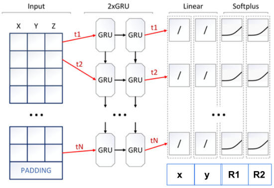
Figure 2.
Main scheme of the TrackNET neuromodel.
Unfortunately, there is a drawback to the TrackNET due to its local nature. The locality means that the model sees only one particular track candidate during the prediction phase and cannot rebuild it in time. Therefore, it can give a lot of false positives, which leads to the creation of an unacceptably large number of false tracks.
There are two ways to eliminate such false tracks. The first one is proposed in [9] and consists of applying the combined approach, when the track candidates from the TrackNET output consider as an input of the graph neural network (GNN) described in [8]. A GNN can now observe the whole event but by looking only at hits from the potential track candidates, which are presented in the form of a graph. A combination of the two models significantly improves the overall precision of tracking without a high decrease in the recall, and at the same time, it greatly reduces the memory consumption of the GNN model.
The second alternative method for identifying false tracks involves applying a statistical criterion that considers the proximity of the track to a smooth spatial curve. This approach was studied in a joint effort [11] by researchers from al-Farabi Kazakh National University and JINR, who proposed algorithms for filtering out false tracks based on approximating the detected points of the particle trajectory with a spatial helix line and calculating a metric that describes the quality of the approximation. If this metric exceeds a certain threshold, it indicates a poor fit of the candidate track to the particle’s trajectory, suggesting that it is a false track.
Therefore, the main objective of this study is to develop algorithms for the most handy approximation and account for data contamination by fake measurements while also employing parallelization techniques to overcome computational limitations. The study will contribute to this area by providing a new and effective solution to this problem.
3. Methodology
3.1. The Solution of a Nonlinear Problem for the Estimation of Helical Line Parameters
The coordinate system of the SPD tracking detectors is arranged so that the direction of the beam of accelerated particles is the direction of the magnetic field of the SPD. The coordinates of event vertices, i.e., particle collision points, are located along the axis near the origin of the coordinates. Assuming homogeneity of the magnetic field of the detector, the particle trajectories must be close to a helical line, with its axis directed along the Oz axis according to the magnetic field direction. The projection of the helical line onto the plane forms a circle of radius R in the plane, centered at , while the helical line itself extends along the Oz axis with an inclination to the plane defined by an angle with tangent . Because the circle touches the origin, we obtain , which reduces the number of parameters of the helical line to three. Thus, we obtain the helical equations in the form of (1):
To estimate the parameters of the helical line, we used a set of model data of particle trajectory measurements in the magnetic field of the SPD detector, simulated according to the pixel detector scheme without considering background measurements. For each track with n measured points, the values of the helical line parameters R, , and had to be estimated, which is a highly nonlinear problem. Therefore, we first applied a variant of the maximum likelihood method with partial adoption of the approach from [12] by one of the authors to estimate the parameters of the circle R, in the plane, with the normalization of the minimizing functional in the form of (2):
by the approximated gradient of the circle . By dividing (2) by and equating derivatives of R, to zero, we obtain (3):
where .
To simplify the equation, it will take the form (4):
Then, the coefficients in (3) are denoted as (5):
Excluding in the system (3) and making the variable substitution , where , we obtain the fourth-degree Equation (6):
with the coefficients (7)
where the coefficients from (7) are determined by formulae (8):
When using Newton’s method with an initial value of zero to solve Equation (6), only one of the required four roots is obtained. However, with just 2–5 iterations, Newton’s method achieves an accuracy of the order of 10.
Calculating , we obtain , from (3) and find .
Then, we can determine the standard deviation of the fitted circle (9):
To calculate the slope of the helical line to the plane, we used linear Equation (1), the maximum likelihood method for which gives an estimate (10):
where , and .
The total root mean square (rms) error of the fitted helical line is calculated as follows (11):
We are going to use this rms range to create a criterion for evaluating the quality of the tracking procedure.
3.2. Dataset Description
The iterative method obtained in the previous section made it possible to estimate the helical line parameters for the model events of the SPD experiment.
For the experiments, certain statistical parameters were calculated for the readout data:
- Number of events: 1000;
- Numbering of events: from 1 to 1000;
- Number of tracks in each event: from 5 to 61.
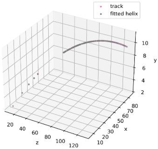
Figure 3.
Normal track (track 10).
Figure 4.
Track with discontinuities (track 21).
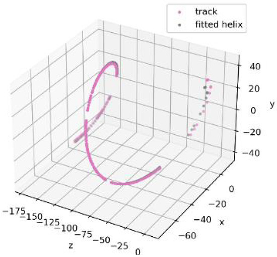
Figure 5.
Track repeatedly twisted (track 26).
The figures presented do not contain any fake hits.
However, to obtain more realistic simulations, it is necessary to include fake hits in the data for each detector station. Because the exact distribution of fake hits is not yet known during the design stage of the SPD setup, it was proposed to distribute them uniformly based on the position of each station. Figure 6 and Figure 7 demonstrate that the addition of only 10 fake hits leads to a noticeable deviation in the results of helical track fitting.
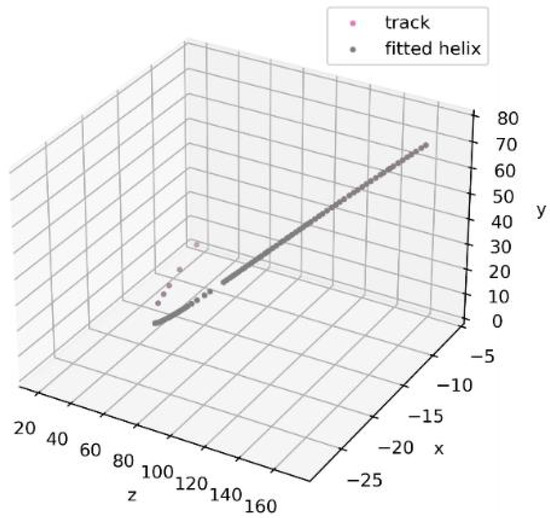
Figure 6.
Track with fake hits, a sample of fitted trajectory with no noise.
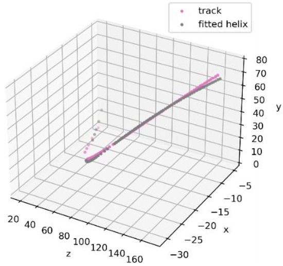
Figure 7.
Track with fake hits, the same track sample fitted with 10 additional noisy hits.
To compare the effect of noise levels on our chosen criterion, we further used 3 levels of noise for the model data of each station: 0, 100, and 1000 fake hits.
3.3. The Data Processing Strategy
The data processing strategy includes selecting the most optimal value through a preliminary clustering of all candidate tracks based on the proximity of their corresponding values. The most populated cluster then chosen to estimate the value for tracks in that cluster is the most significant.
To extend this strategy to three levels of data contaminated by fake measurements, three stages of data processing were used. In the first stage, which did not involve any fake hits, all tracks in the dataset were clustered using as a measure of track proximity. X-means clustering [12] was applied to these data, with the clustering conducted in two phases. In the first phase, initial clustering centers were obtained using the KMeans++ algorithm, which provides a close estimate to the optimal centers due to its probabilistic approach. The remaining clustering relied on the X-means algorithm, which refines clustering decisions by computing Bayesian Information Criterion at each step of the algorithm. The goal was to achieve a stable approach for determining false tracks, i.e., tracks that do not correspond to a correct particle trajectory. The results of the first stage are presented in Table 1.

Table 1.
Clustering results for the first 10 clusters with the lowest chi-squared values.
A total of 30 clusters were obtained, and the results of the clustering analysis for the first 10 clusters with the lowest chi-squared values are shown in Table 1. Analysis of the clusters based on mean and number of elements revealed that 83% of the tracks belonged to cluster 1, which had the lowest mean and standard deviation values for . The other clusters showed noticeably higher errors in the helical fitting procedure for the tracks. A visual comparison of the tracks also revealed the differences between the clusters. The “good” tracks in cluster 1 showed no significant discontinuities or spirals. This strong correlation between track properties and the value of , which represents the quality of the helix line fitting for each track, led to the idea of using to filter out false tracks that can occur during neural network reconstruction.
The first stage of our work involved developing a parallelization approach to speed up the procedure of false track rejection using neural network tracking.
3.4. Boosting Algorithm Efficiency for Accurate Track Elimination through Parallelization Techniques
According to references [13,14], parallelization within an event involves executing multiple cores simultaneously from multiple event queues to achieve additional parallelism. Although the order of kernel execution within a sector must be maintained, different sectors can be distributed across multiple queues, allowing all cores for one sector to be put in the same queue. This technique can be implemented up to the number of queues equal to the number of sectors, but it is recommended to match the number of queues with hardware constraints for optimal performance.
On the other hand, the HLT GPU framework allows for the execution of kernels for multiple events simultaneously as a simpler and completely different approach to parallelization, as stated in reference [15]. Each independent processing component performs track reconstruction on the same GPU if there is enough GPU memory available for all of them. However, this technique can increase the memory requirement by the number of simultaneous queues, although it effectively loads the GPU.
In our study, for greater generality, two approaches were used to approximate the found candidate tracks. In the first approach, a spatial helix was fitted; in the second, a spatial polynomial of the third degree. In Algorithm 1 proposed for computing optimal helix-loop parameters in parallel, we used running parallel threads, where each thread performs a fitting procedure for events assigned to the threads according to the circular round-robin procedure. A schematic of the parallel Algorithm 1 is shown in Figure 8.
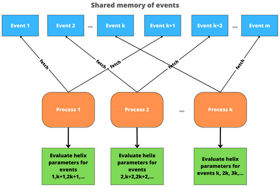
Figure 8.
Schematic diagram of the parallel Algorithm 1.
| Algorithm 1 Track Reconstruction |
| Require: DataFrame D containing hit coordinates , event and station identifiers, and track number |
| Ensure: Labeled tracks T |
| 1: Load TrackNETv2.1 model |
| 2: function GenerateCandidates(D) |
| 3: Candidate tracks [] |
| 4: for to do |
| 5: |
| 6: TrackNetv2.1(h) |
| 7: add c to C |
| 8: end for |
| 9: return C |
| 10: end function |
| 11: GenerateCandidates(D) |
| 12: function LabelTracks(C) |
| 13: Labeled tracks [] |
| 14: for c in C do |
| 15: fit helix to c |
| 16: calculate value for fitted helix |
| 17: if < threshold then |
| 18: label c as correct |
| 19: else |
| 20: label c as false |
| 21: end if |
| 22: add c to T |
| 23: end for |
| 24: return T |
| 25: end function |
| 26: LabelTracks(C) |
All tracks table contains the coordinates of the top of the event x, y, z, the identity number of the event N, the station number s, the detector number d, and the track number T within the event. Large number of tracks formed by different events necessitates improving the performance of the optimal helical parameter fitting process for each of the tracks. Thus, in our implementation, we propose a partitioning algorithm that uses multi-threaded computation to divide the workload among processing threads. The partitioning algorithm is based on the round-robin procedure that uses the approach of sequential execution of tasks by parallel threads. If we have k threads, tasks are distributed in such a way that the first thread will compute parameters for the first track from the dataset, the second thread will compute parameters for the second track, and so on, until we reach the k-th element (with a thread k), and in circular fashion, -th element will be processed by the first thread again, and so on, until all the elements of the table are processed.
4. Results and Discussion
The Algorithm 1 speed-up and performance is shown in Figure 9. Looking at the graph, we can notice that the speed-up of the algorithm is achieved and the processing time improves with the increase in the number of threads.
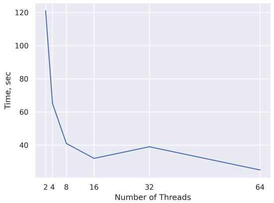
Figure 9.
Execution time of parallel Algorithm 1 as a function of thread count.
In this sub-subsection we introduce parallel Algorithm 2, which is based on different approach of fitting track trajectory [15].
| Algorithm 2 Polynomial Fit Method |
| Require: All Tracks Table with x, y, z, N, s, d, and T |
| 1: for each track in All Tracks Table do |
| 2: Compute initial parametrization u using centripetal method |
| 3: Define polynomials , , of degree k |
| 4: for each parameter in u do |
| 5: Compute n using Equation (12) |
| 6: Initialize search interval around |
| 7: repeat |
| 8: Apply Golden Ratio search on interval |
| 9: Update a and b based on Golden Ratio search |
| 10: Compute residuals and update , , |
| 11: until convergence criterion is met or maximum iterations are reached |
| 12: end for |
| 13: Compute final polynomials , , |
| 14: end for |
| Ensure: Fitted polynomial parameters for each track |
4.1. Parallel Algorithm 2
In reality, due to inhomogeneity of the magnetic field of the SPD setup and the influence of various factors distorting the particle trajectory, such as Coulomb scattering, etc., the helical line in space ceases to adequately describe the trajectory. In addition, the iterative nonlinear fitting method described above proves to be slower than the linear approach and more complicated to parallelize. Therefore, another method using a third-degree spatial polynomial was applied.
Assuming we have a set of n knot points , where , the parametrization is made, which associates knot points with parameters . Based on that parametrization, we can find an approximation curve, . Each of the approximation curves is represented by a polynomial function of a certain degree k.
The idea is to fit the curve such that the distance to the knot points from the curve is minimized given the parametrization u. To perform this step, we rely on the method of the least squares, where the sum of squares of residuals of the curve points and their corresponding knot points are minimized.
To iteratively approximate the parameters, it is required to make an initial parametrization, which is based on the centripetal parametrization approach (see formula below):
The input parameters for the algorithm are the same as for Algorithm 1 and contain the coordinates of the event node x, y, z, the event identification number N, the station number s, the detector number d, and the track number T within the event.
The algorithm is based on fitting spatial polynomials of the third degree to track coordinates. To find new estimates of parameters at each iteration, the Golden Ratio search method is used for locally minimizing the approximation error computed as described above from the residual values of knot points and the corresponding curve. Due to the more efficient computational cycle, this algorithm is characterized by a fast computation procedure and is therefore less computationally demanding.
Because the Golden search method demands a certain number of iterations until convergence, we need to determine the optimal number of iterations for convergence to the required calculation accuracy. To this end, we have applied convergence estimation methods according to the formula
Using this formula, we can estimate the number of iterations n that algorithm will take to find a minimum on the given interval between endpoints and for each corresponding dimension in the 3D plane for the estimated parameter value . The Golden Ratio search is an effective way of gradually reducing the interval for finding the minimum. Ensuring that the estimated minimum falls within the range defined by the two points immediately adjacent to the point with the lowest estimated value is crucial, regardless of the number of estimated points.
Next, polynomials are constructed using standard quadratic error minimization techniques:
4.2. Comparison of Performances for Two Algorithms
By comparing the two algorithms, the main aspects of each method can be highlighted as shown in Table 2.
Table 2.
Aspects of two algorithms.
Thus, it can be observed that Algorithm 2 appears to be superior when evaluated against the fundamental performance criteria provided earlier.
Parallelization is based on the multiprocessing library in the Python programming language. As an implementation, an algorithm for splitting the array of events into threads was used. Figure 10 illustrates how the number of threads affects the run-time of the parallel algorithm.
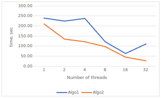
Figure 10.
Comparative running times of the two proposed parallel algorithms.
The algorithm was tested on a compute node with multiple cores and the following specifications: 32 cores, 64 Gb of memory, an AMD Ryzen processor, and 2 Tb of disk memory (SSD).
This system supports up to 64 parallel threads. In our experiment, we tested the computation time results for the sequential code without parallelization, with 2, 4, 8, 16, 32, and 64 parallel threads.
Our experiment used a track table consisting of 42,102 tracks. The average execution time of a subroutine to calculate the optimum helix parameters for 1 track from the whole set is approximately 0.5 × 10 s.
The results demonstrate a significant speed-up of up to six-fold. However, there is some decline in the speed-up achieved for higher thread numbers due to the additional memory fill factor. It is worth noting that this algorithm may face limitations in processing large datasets with high memory requirements.
4.3. Neural Network Algorithm for Track Recognition and Its Performance Results with False Tracks before and after Applying the Track Rejection Criterion
For the training, we used the TrackNET model as a software application that employs a deep recurrent neural network for local tracking. This network retrieves each track individually, progressing station by station. The model’s specifications have been thoroughly explained. The efficacy of track recovery is determined by evaluating recall and precision, the two most commonly used metrics. Recall denotes the proportion of true tracks that are recovered entirely, while precision indicates the proportion of actual tracks among all the tracks detected by the model.
To train the neural network, 50,000 model SPD events of simplified geometry were used. Each sample event, apart from the tracks (on average 5), contained false (noise) tracks, with an average of 60 false tracks per event.
The trained model is able to reconstruct 90% or more tracks. However, the neural network also outputs false tracks along with real tracks, with the number of false tracks being much higher. Therefore, in the total number of tracks from the dataset, reconstructed with TrackNETv3, only 2% are true tracks.
In order to increase the share of true tracks in the total number of all reconstructed tracks, we used a value of as a criterion for elimination. A false track is far enough away from the reconstructed helix, as opposed to a true track, that if the threshold for is chosen correctly, only false tracks will be screened out among all reconstructed tracks.
The screening threshold was calculated under ideal conditions, on a sample containing only true tracks, as the average value of plus 3 standard deviations, so that its value is 0.023. The distribution of for both true and false tracks is shown in Figure 11 and Figure 12.
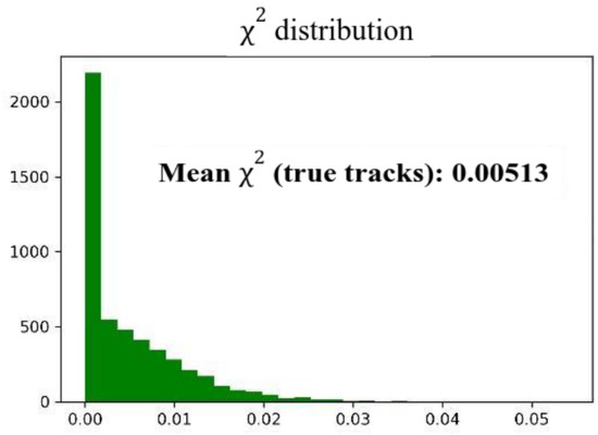
Figure 11.
Distribution of for true tracks.
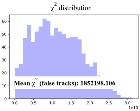
Figure 12.
Distribution of for false tracks.
Figure 13 illustrates how the recall and precision metrics vary with changes in the false track rejection criterion.
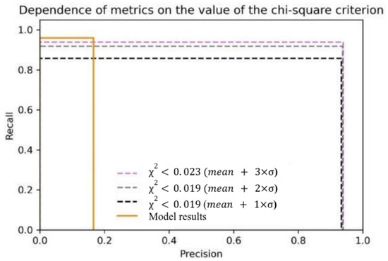
Figure 13.
Dependence of the recall and precision metrics on the value of the screening criterion.
In this way, the track sifting experiment increased the accuracy metric from 0.16 to 0.93. At the same time, the recall metric did not fall below 0.93. All the experiments were conducted using Ariadne library tools [16]. The resource calculations were performed using the heterogeneous computing platform HybriLIT (LIT, JINR) [17].
4.4. False Track Rejection with Contaminated Data
Due to bias in the original dataset, the model has some limitations in terms of the potentially poor reconstruction of true tracks in the presence of highly noisy data that contain a lot of false hits. Actual experimental data show that, on average, the number of false hits in each detector can reach up to n to , where n represents the total number of tracks per event. Therefore, to test the introduced criteria for track clustering based on the chi-squared measure, we propose modeling more realistic samples and adding noisy hits to the dataset, corresponding to two different noise levels. The first noise level will contain 100 false hits per station, while the higher noise level will contain 1000 false hits.
The comparative clustering results are presented in Table 3.
Table 3.
Center cluster chi-squared depending on zero level of noise, 100 false hits, 1000 false hits.
The model takes a pandas DataFrame object [18] containing information on events, with columns for x, y, z, the event number, the station number, and the track number (or −1 for fake hits) as input.
The algorithm produces candidate tracks as output, which are then converted into the hit index format and compared with the real tracks based on complete coincidence. The Ariadne library was used to train and test the model [16].
The algorithm is designed to improve the reconstruction of track trajectories in particle collision experiments. One sub-task is finding parameters to fit a helical line to a set of points along the track trajectory, which allows for filtering out false tracks by a proposed chi-squared error criterion. To speed up the track reconstruction process, we proposed a basic approach to parallelize the task of finding helix parameters for multiple tracks simultaneously. This approach significantly improves performance, as shown in the experimental results. The track reconstruction algorithm proposed in our paper consists of three major steps:
- The input data in the form of a DataFrame containing hit coordinates , event and station identifiers, and the track number are fed into the neural network.
- The network generates candidate tracks using the TrackNETv2.1 model.
- A thresholding procedure is applied to cluster the track candidates based on the chi-squared values obtained from fitting a helix to each trajectory. The tracks are then labeled as either false or correct.
The goal of the algorithm is to take in a DataFrame containing hit coordinates, event and station identifiers, and the track number and generate labeled tracks. The input DataFrame is denoted as D and the output labeled tracks are denoted as T.
The algorithm begins by loading the TrackNETv2.1 model, which will be used to generate candidate tracks. The function GenerateCandidates is then called to generate candidate tracks from the input DataFrame D. This function loops over each hit in D and applies the TrackNETv2.1 model to generate a candidate track for each hit. The candidate tracks are stored in a list called C.
Once the candidate tracks are generated, the function LabelTracks is called to apply a thresholding procedure to cluster the track candidates based on the chi-squared values obtained from fitting a helix to each trajectory. This function loops over each candidate track in C and fits a helix to the track. The chi-squared value is then calculated for the fitted helix. If the chi-squared value is below a certain threshold, the track is labeled as correct; otherwise, it is labeled as false. The labeled tracks are stored in a list called T.
The final output of the algorithm is the labeled tracks T.
Overall, the algorithm is a pipeline for track reconstruction, starting with raw hit data and generating labeled tracks using a neural network model and a thresholding procedure.
The results presented in Table 4 demonstrate that the proposed approach is capable of detecting correct tracks with high levels of recall and precision. Recall is calculated as the ratio of the number of real tracks detected by the model to the number of real tracks in the dataset. Precision is calculated as the ratio of the number of real tracks detected by the model to the total number of reconstructed tracks. The testing was performed on a DGX cluster equipped with A100 GPU with 40 Gb and 1 Tb memory, as well as a Dual 64-Core AMD CPU, using a dataset of 10,000 events. The training process took around 25.6 h to complete, with 500 epochs for training on a dataset comprising 100 noisy points and slightly more for a dataset comprising 1000 fake points.
Table 4.
Recall and precision with fake hits (100 and 1000 hits per station) and without fake hits.
In Rusov et al. [9], the authors present a combined approach based on TrackNetv3 and a GNN (graph neural network). The algorithm presented here in this paper describes a different approach to track elimination, where track candidates generated by the model are fed to a parallel track elimination algorithm with the same aim to reduce a false positive rate inherent to the TrackNetv2 model. We present a novel procedure with a clustering of track candidates based on chi-squared criteria. This approach demonstrated to be highly effective to reduce the false positive rate, as can be witnessed by the presented results. Comparing these two approaches, we can conclude that in terms of efficiency (recall and precision) both algorithms show similar results. Moreover, our algorithm displays a fast inference time (calculation time for 1 event) due to the parallel nature of the computation and less computational workload.
5. Conclusions and Outlook
This paper presents an approach to improve the quality and speed of tracking, which is a key procedure for data processing in high-energy physics experiments. This approach realizes an optimal balance between the efficiency of track reconstruction and the speed of this procedure on modern multicore computers. For this purpose, a threshold criterion of reconstruction quality is introduced, which uses the rms error of spiral and polynomial fitting for the measurement sets recognized by the neural network as the next track candidate. The right choice of the threshold allows us to keep the recall and precision metrics of the neural network track recognition efficiency at an acceptable level for physicists (although these metrics inevitably decrease with increasing data contaminations). In addition, it was possible to increase the speed of the entire chain of programs six-fold by paralleling the algorithm, reaching a rate of 2000 events per second, even with maximum noisy input data. This speed achieved on a DGX cluster equipped with A100 GPU with 40 Gb and 1 Tb memory, as well as with a Dual 64-Core AMD CPU significantly exceeds the results obtained in [19] on Nvidia V100 GPU taking into account their performance differences. Further multiple acceleration of the algorithm is supposed to be achieved by translating the program that implements it into C++.
Author Contributions
Conceptualization, G.O., M.M. and N.B.; methodology, G.O.; software, A.S.; validation, G.A. and G.O.; formal analysis, M.K., G.A. and A.S.; investigation, G.A. and G.O.; resources, G.O. and A.S.; data curation, M.K.; writing—original draft preparation, G.A. and A.S.; writing, G.A.; review and editing, G.O.; visualization, A.S.; supervision, M.M.; project administration, M.M. All authors have read and agreed to the published version of the manuscript.
Funding
This research was funded by the Program No. BR10965191 (Complex Research in Nuclear and Radiation Physics, High Energy Physics and Cosmology for the Development of Competitive Technologies) of the Ministry of Education and Science of the Republic of Kazakhstan.
Data Availability Statement
Not applicable.
Acknowledgments
The work was supported by the Program No. BR10965191 (Complex Research in Nuclear and Radiation Physics, High Energy Physics and Cosmology for the Development of Competitive Technologies) of the Ministry of Education and Science of the Republic of Kazakhstan.
Conflicts of Interest
The authors declare no conflict of interest.
Abbreviations
The following abbreviations are used in this manuscript:
| HEP | High-Energy Physics |
| JINR | Joint Institute for Nuclear Research |
| CERN | Conseil Europeen pour la recherche Nucleaire (fr.) or The European Organization |
| for Nuclear Research | |
| BNL | Brookhaven National Laboratory |
| LHC | The Large Hadron Collider of CERN |
| NICA | Nuclotron-based Ion Collider fAcility of JINR |
| RHIC | The Relativistic Heavy Ion Collider of BNL |
| EIC | The Electron-Ion Collider |
| SPD | Spin Physics Detector on NICA Collider |
| BM@N | Baryonic Matter at Nuclotron—the fixed-target experiment on NICA collider |
References
- Abazov, V.M.; Abramov, V.; Afanasyev, L.G.; Akhunzyanov, R.R.; Akindinov, A.V.; Akopov, N.; Alekseev, I.G.; Aleshko, A.M.; Alexakhin, V.Y.; Alexeev, G.D.; et al. Conceptual Design of the Spin Physics Detector. arXiv 2021, arXiv:2102.00442. [Google Scholar] [CrossRef]
- Frühwirth, R. Application of Kalman Filtering to Track and Vertex Fitting. Nucl. Instrum. Meth. A 1987, 262, 444–450. [Google Scholar] [CrossRef]
- Denby, B. Neural Networks and Cellular Automata in Experimental High Energy Physics. Comput. Phys. Commun. 1988, 49, 429–448. [Google Scholar] [CrossRef]
- Hopfield, J.J. Neural Networks and Physical Systems with Emergent Collective Computational Abilities. Proc. Nat. Acad. Sci. USA 1982, 79, 2554–2558. [Google Scholar] [CrossRef] [PubMed]
- Hopfield, J.J.; Tank, D.W. Computing with Neural Circuits: A Model. Science 1986, 233, 625–633. [Google Scholar] [CrossRef] [PubMed]
- Gyulassy, M.; Harlander, M. Elastic Tracking and Neural Network Algorithms for Complex Pattern Recognition. Comput. Phys. Commun. 1991, 66, 31–46. [Google Scholar] [CrossRef]
- Farrell, S.; Calafiura, P.; Mudigonda, M.; Anderson, D.; Vlimant, J.R.; Zheng, S.; Bendavid, J.; Spiropulu, M.; Cerati, G.; Gray, L.; et al. Novel Deep Learning Methods for Track Reconstruction. arXiv 2018, arXiv:1810.06111. [Google Scholar] [CrossRef]
- Ju, X.; Murnane, D.; Calafiura, P.; Choma, N.; Conlon, S.; Farrell, S.; Xu, Y.; Spiropulu, M.; Vlimant, J.R.; Aurisano, A.; et al. Performance of a Geometric Deep Learning Pipeline for HL-LHC Particle Tracking. Eur. Phys. J. C 2021, 81, 1–14. [Google Scholar] [CrossRef]
- Rusov, D.; Nikolskaia, A.; Goncharov, P.V.; Shchavelev, E.; Ososkov, G. Deep Neural Network Applications for Particle Tracking at the BM@N and SPD Experiments. Available online: https://inspirehep.net/files/804ee777e07426ddac430fd984d12ade (accessed on 15 June 2023).
- Gated Recurrent Unit. Available online: https://en.wikipedia.org/wiki/Gated_recurrent_unit (accessed on 14 March 2023).
- Amirkhanova, G.A.; Ashimov, Y.K.; Goncharov, P.V.; Zhemchugov, A.S.; Mansurova, M.Y.; Ososkov, G.A.; Rezvaya, Y.P.; Shomanov, A.S. Application of the Maximum Likelihood Method to Estimate the Parameters of Elementary Particle Trajectories in the Reconstruction Problem of the Internal Detector of the SPD NICA Experiment. In Proceedings of the Information and Telecommunication Technologies and Mathematical Modelling of High-Tech Systems, Moscow, Russia, 18–22 April 2022; pp. 335–341. [Google Scholar]
- Pelleg, D.; Moore, A.W. X-means: Extending k-means with Efficient Estimation of the Number of Clusters. Mach. Learn. 2002, 1, 727–734. [Google Scholar]
- Canetti, L.; Drewes, M.; Shaposhnikov, M. Matter and Antimatter in the Universe. New J. Phys. 2012, 9, 095012. [Google Scholar] [CrossRef]
- LHCb Collaboration. Framework TDR for the LHCb Upgrade: Technical Design Report; CERN: Geneva, Switzerland, 2012; Tech. Rep. CERNLHCC-2012-007. LHCb-TDR-12. [Google Scholar]
- Parametric Curve Fitting with Iterative Parametrization. Available online: https://meshlogic.github.io/posts/jupyter/curve-fitting/parametric-curve-fitting/ (accessed on 14 March 2023).
- Ariadne. Available online: https://github.com/t3hseus/ariadne (accessed on 14 March 2023).
- Adam, G.; Bashashin, M.; Belyakov, D.; Kirakosyan, M.; Matveev, M.; Podgainy, D.; Sapozhnikova, T.; Streltsova, O.; Torosyan, S.; Vala, M.; et al. IT-Ecosystem of the HybriLIT Heterogeneous Platform for High-Performance Computing and Training of IT-Specialists. In Proceedings of the CEUR Workshop, Avignon, France, 10–14 September 2018; Volume 2267, pp. 638–644. [Google Scholar]
- Stepanek, H. Thinking in Pandas; Apress: Berkeley, CA, USA, 2020. [Google Scholar] [CrossRef]
- Anderson, D.J. The HEP.TrkX Project. Approaching Charged Particle Tracking at the HL-LHC with Deep Learning, for Online and Offline Processing. Available online: https://indico.cern.ch/event/587955/contributions/2937540/ (accessed on 14 March 2023).


Disclaimer/Publisher’s Note: The statements, opinions and data contained in all publications are solely those of the individual author(s) and contributor(s) and not of MDPI and/or the editor(s). MDPI and/or the editor(s) disclaim responsibility for any injury to people or property resulting from any ideas, methods, instructions or products referred to in the content. |
© 2023 by the authors. Licensee MDPI, Basel, Switzerland. This article is an open access article distributed under the terms and conditions of the Creative Commons Attribution (CC BY) license (https://creativecommons.org/licenses/by/4.0/).