2.1. A New Approach: Continued Fractions with Splines
In previous contributions [
8,
9], a memetic algorithm was employed to find the approximations. Here, we present another method to fit continued fraction representations by iteratively fitting splines.
Splines provide a regression technique that involves fitting piecewise polynomial functions to the given data [
15]. The domain is partitioned into intervals at locations known as “knots”. Then, a polynomial model of degree
n is separately fitted for each interval while generally enforcing boundary conditions, including the continuity of the function and continuity of the first
-order derivatives at each of the knots. Splines can be represented as a linear combination of basis functions, of which the standard is the B-spline basis. Thus, fitting a spline model is equivalent to fitting a linear model of basis functions. We refer to Hastie et al. [
16] for the particular definition of the B-spline basis.
First, when all the functions
, we have a
simple continued fraction representation for all
i, which we can write as
Note that for a term
we say that it is at a “depth” of
i.
Finding the best values for the coefficients in the set of functions
can be addressed as a nonlinear optimization problem as in [
8,
9]. However, despite the great performance of that approach we aim to introduce a faster variant that can scale well to larger datasets such as this one.
Towards that end, and thinking about the scalability, we fit the model iteratively by depth as follows: we first consider only the first term
at depth 0, ignoring all other terms. We fit a model for the first term using the predictors
and target
. Next, we consider only the first and second depths, with the terms
and
, ignoring the rest. We then fit
using the previously fit model for
. For example, truncating the expansion at depth 1, we have
Thus, we fit using the predictors and the target . We label this target as . We repeat this process, fitting a new model by truncating at the next depth by using the models fit from previous depths and iterations.
We have that at depth , the target for the model is , where is the residual of the previous depth’s model, .
One notable characteristic of this approach is that if any model , evaluates to 0, then we will have a pole in the continued fraction, which is often spurious. To remedy this, we modify the structure of the fraction such that each fitted , is encouraged to be strictly positive on the domain of the training data. To do this, we add a constant to when calculating the target , where . Thus, the targets for are all non-negative, encouraging each , , to be strictly positive. For example, for , we would have that the target . Of course, we must then subtract from in the final continued fraction model.
We have found that data normalization often results in a better fit using this approach. It is sufficient to simply divide the targets uniformly by a constant when training and multiply by the same constant for prediction. We denote this constant parameter .
A good choice of the regression model for each
is a spline since they are well-established. For reasons stated in the next section, the exception is the first term
, which is a linear model. We use an additive model to work with multivariate data where each term is a spline along a dimension. That is, given
m predictor variables, we have that
for each term
,
, where each function
is a cubic spline along variable
j, that is,
is a piecewise polynomial of degree 3 and is a function of variable
j.
We implement the splines with a penalized cubic B-spline basis, that is,
, where each
is one of
k cubic B-spline basis functions along dimension
j and corresponds to one of
k knots. We use the following loss function
, i.e.,
where
is the matrix of cubic B-spline basis functions for all variables,
is the vector of all of the weights, and
is the associated second derivative smoothing penalty matrix for the basis for the spline
. This is standard for spline models [
16]. The pseudocode for this approach is shown in Algorithm 1.
| Algorithm 1: Iterative CFR using additive spline models with adaptive knot selection |
![Algorithms 16 00382 i001]() |
2.2. Adaptive Knot Selection
The iterative method of fitting continued fractions allows for an adaptive method of selecting knot placements for the additive spline models. For the spline model at depth , we use all of the knots of the spline model at depth . Then, for each variable, we place k new knots at the unique locations of the k samples with the highest absolute error from the model at depth . As the points with the highest error are likely to be very close to each other, we impose the condition that we take the samples with the highest error, but they must have alternating signs.
In this way, we select
k knots for
and
, with the first knot at the location of the sample with the highest absolute error computed from the model
. For the rest of the knots, the
knot is selected at the sample’s location with the next highest absolute error after the sample used for the
knot, and only if the sign of the (non-absolute) error of that sample is different from the sign of the (non-absolute) error of the sample used for the
knot. Otherwise, we move on to the next highest absolute error sample, and so on, until we fulfill this condition. This knot selection procedure is shown in Algorithm 2. Note that we let
be a linear model, as there is no previous model from which to obtain the knot locations.
| Algorithm 2: SelectKnots (Adaptive Knot Selection) |
![Algorithms 16 00382 i002]() |
The goal of using additive spline models with the continued fraction is to take advantage of the continued fraction representation’s demonstrated ability to approximate general functions (see the discussion on the relationship with Padé approximants in [
9]). The fraction’s hierarchical structure allows for the automatic introduction of variable interactions, which is not included individually in the additive models that constitute the fraction. The iterative approach to fitting makes for a better knot selection algorithm.
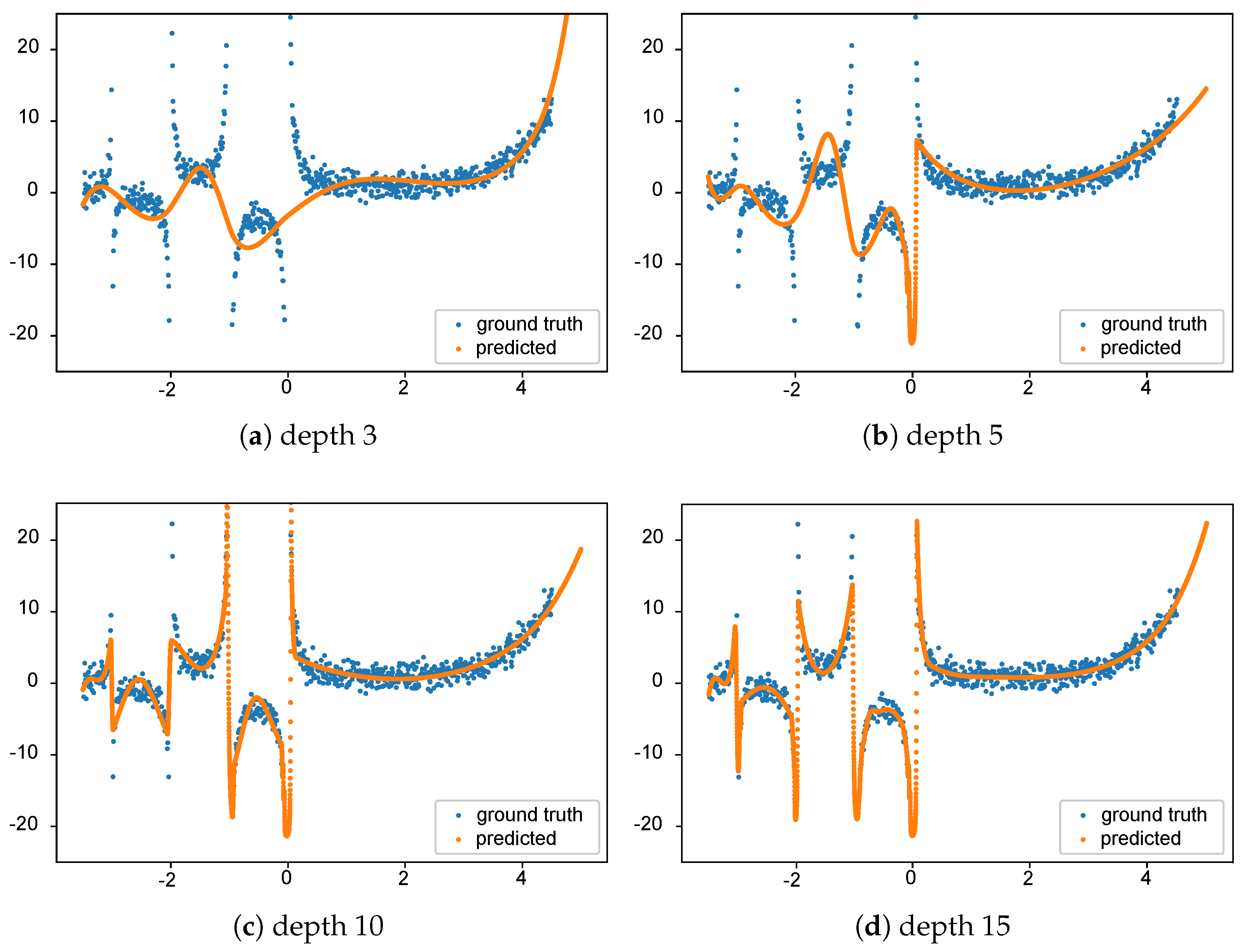
An example of this algorithm modeling the well-known gamma function (with standard normally distributed noise added) is demonstrated in
Figure 1. Here, we show how the fitting to gamma is affected by different values of depths (3, 5, 10, 15) in the
Spline Continued Fraction. As desired, it is evident from the figure that the
Spline Continued Fraction with more depth has a better fit with the data.
2.3. Data and Methods Used in the Study
We used the superconductivity dataset from Hamidieh [
7], available from the UCI Machine Learning repository (
https://archive.ics.uci.edu/ml/datasets/Superconductivty+Data, accessed on 11 September 2020). The website contains two files. In this work, we only used the
train.csv file, which contains information on 21,263 superconductors, including the critical temperature and a total of 81 attributes for each of them.
This dataset on superconductors utilizes elemental properties to predict the critical temperature (). The data extraction process involves obtaining ten features from the chemical formula for each of the eight variables, which include Atomic Mass, First Ionization Energy, Atomic Radius, Density, Electron Affinity, Fusion Heat, Thermal Conductivity, and Valence. This results in a total of 80 features. Additionally, the dataset includes one extra feature representing the count of elements present in the superconductor. The dataset encompasses both “oxides” and “metallic” materials, but excludes elements with atomic numbers greater than 86. After performing thorough data preparation and cleaning steps, the final dataset consisted of 21,263 samples, each described by 81 features.
Regarding the elemental distributions of the superconductors in the dataset, Oxygen constitutes approximately 56% of the total composition. Following Oxygen, the next most abundant elements are Copper, Barium, Strontium, and Calcium. As many of the research group’s primary interest is in iron-based superconductors, the following information is likely to be of significant interest to them. Within this dataset, Iron is present in about 11% of the superconductors, with a mean critical temperature () of 26.9 ± 21.4 K. On the other hand, the mean for non-iron-containing superconductors is 35.4 ± 35.4 K. Looking at the overall distribution of values, it is found to be right-skewed, with a noticeable peak centered around 80 K.
For a more detailed understanding of the data generation, feature extraction process, and specific characteristics of the dataset, readers can refer to Hamidieh’s original contribution in [
7].
We conducted two main studies to assess the generalization capabilities of many regression algorithms. We denote these as Out-of-Sample and Out-of-Domain, respectively. For the Out-of-Sample study, the data were randomly partitioned into two thirds training data and one third test data. Each model was fitted to the training data, and the RMSE was calculated on the separated test portion of the data.
For the Out-of-Domain study, the data were partitioned such that the training samples were always extracted from the set of samples with the lowest 90% of critical temperatures. For the test set, the samples come from the highest 10% of critical temperatures. It turned out that the lowest 90% had critical temperatures < 89 K, whereas the highest 10% had temperatures greater than or equal to 89 K that ranged from 89 K to 185 K (we highlight that the range of variation of the test set is more than that of the training set, making the generalization task a challenging one). For each of the 100 repeated runs of the Out-of-Domain test, we randomly took half of the training set (from lowest 90% of the observed value) to train the models and the same ratio from the test data (from 10% of the highest actual value) to estimate the model performance. The Out-of-Domain study allowed us to assess the capacity of several regression models in terms of “prediction” on a set of materials with higher critical temperatures, meaning that in this case generalization is strictly connected to the extrapolation capacity of the fitted models. We executed both the Out-of-Sample and Out-of-Domain tests 100 times to help validate our conclusions with statistical results.
The
Spline Continued Fraction model had a depth of 5, five knots per depth, a normalization constant of 1000, and a regularization parameter
of 0.5. These parameters resulted from a one-dimensional nonlinear model fitting to problems such as the gamma function with noise (already discussed in
Figure 1) and others, such as fitting the function
. The parameters were selected empirically using these datasets; no problem-specific tuning on the superconductivity datasets was conducted.
The final model was then iteratively produced by beginning at a depth of 1 and increasing the depth by one until the error was greater than that observed for a previous depth (which we considered as a proxy for overfitting the data).
To evaluate the performance of the
Spline Continued Fraction (
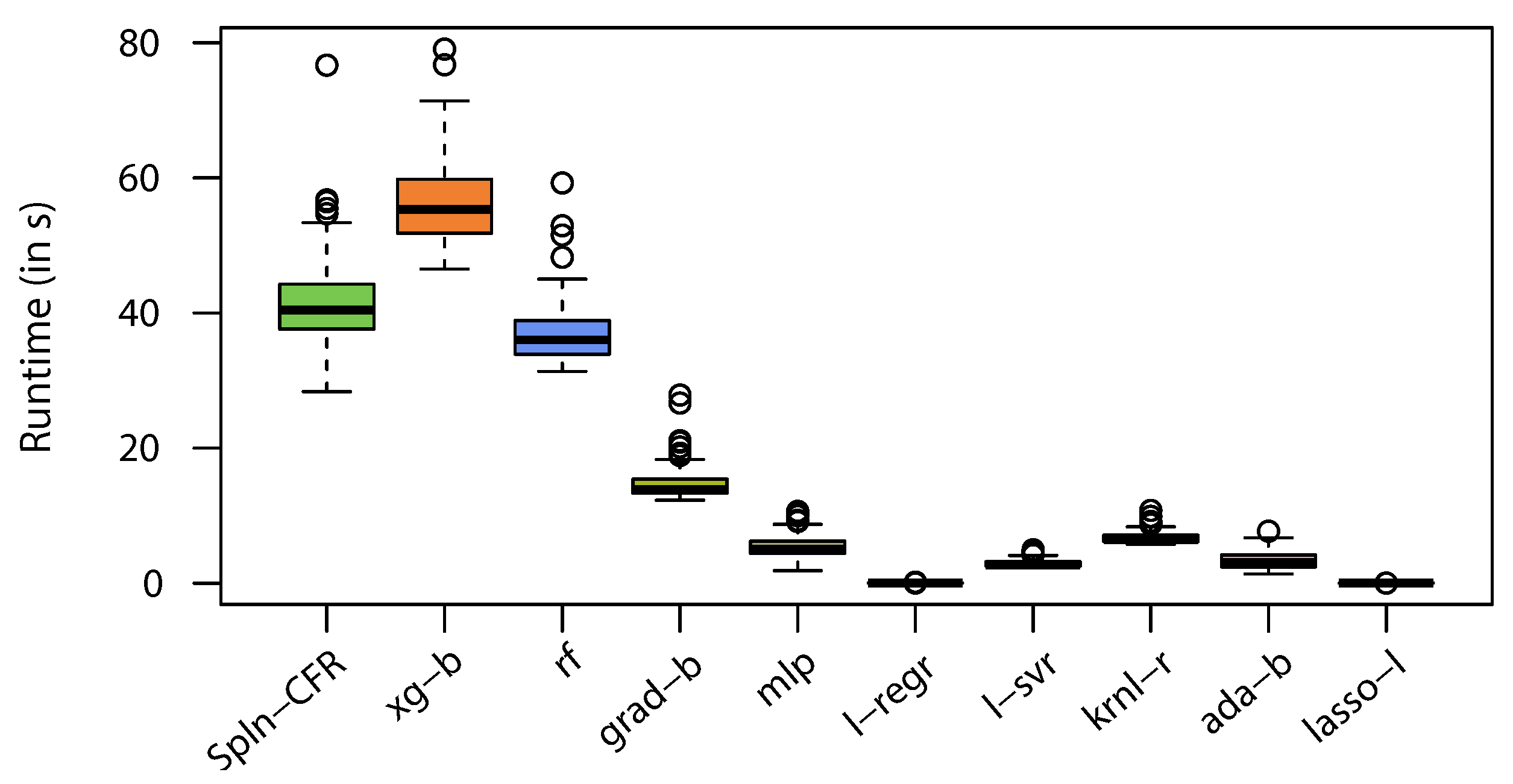
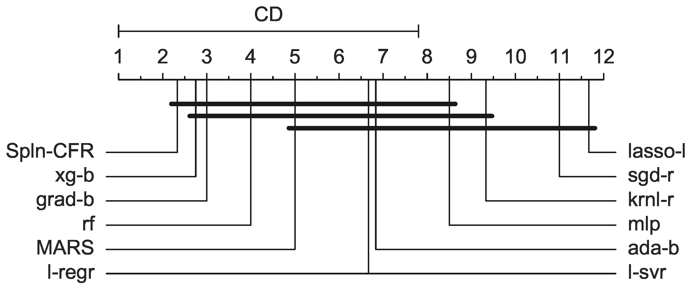
Spln-CFR) introduced in this paper with other state-of-the-art regression methods, we used a set of eleven regressors from two popular Python libraries, namely, the
XGBoost [
17] and
Scikit-learn [
18] machine learning libraries. The names of the regression methods are listed as follows:
AdaBoost (ada-b)
Gradient Boosting (grad-b)
Kernel Ridge (krnl-r)
Lasso Lars (lasso-l)
Linear Regression (l-regr)
Linear SVR (l-svr)
MLP Regressor (mlp)
Random Forest (rf)
Stochastic Gradient Descent (sgd-r)
XGBoost (xg-b)
The
XGBoost code is available as an open-source package (
https://github.com/dmlc/xgboost, accessed on 11 September 2020). The parameters of the
XGBoost model were the same as those used in Hamidieh (2018) [
7]. We kept the parameters of the other machine learning algorithms the same as the Scikit defaults.
All executions of the experiments were performed on an Intel
Core
i7-9750H hexcore-based computer with hyperthreading and 16 GB of memory running a Windows 10 operating system. We used Python v3.7 to implement the
Spline Continued Fraction using the pyGAM [
19] package. All experiments were executed under the same Python runtime and computing environment.


