Path Algorithms for Contact Sequence Temporal Graphs ^†

Abstract

This paper proposes a new time-respecting graph (TRG) representation for contact sequence temporal graphs. Our representation is more memory-efficient than previously proposed representations and has run-time advantages over the ordered sequence of edges (OSE) representation, which is faster than other known representations. While our proposed representation clearly outperforms the OSE representation for shallow neighborhood search problems, it is not evident that it does so for different problems. We demonstrate the competitiveness of our TRG representation for the single-source all-destinations fastest, min-hop, shortest, and foremost paths problems.

1. Introduction

This paper extends our previous paper on contact sequence temporal graphs [1]. We have extended our previous work mainly by adding two path-finding algorithms to our proposed TRG data structure. Also, we have considered the case when the TRG graph is acyclic and proposed path-finding algorithms that can further benefit from that property.

Temporal graphs are graphs that change over time. Therefore, temporal information is incorporated in the edges or vertices. In this paper, we are only concerned with graphs in which the temporal information is incorporated in the edges. Temporal graphs have applications in modeling a wide range of phenomena, such as communication networks, computational biology, transportation networks, the spread of viruses, social networks, etc. [2,3,4,5,6].

In a contact sequence temporal graph $G=(V,E)$, each edge $e\in E$ has the format $(u,v,t,w)$ where u and v are the source and target vertices, respectively, of the edge; t is its time stamp and w ($w\ge 0$) is the time it takes to get from u to v along this edge. We may begin traveling from u only at the time indicated by the timestamp t. We arrive at v at the time $=t+w$. Contact sequence temporal graphs may have multiple edges with the same source and target vertices, each with a different time stamp and possibly different weight.

An example of a real-life application of contact sequence temporal graphs is transportation networks such as the flight network of a particular airline. The nodes of the contact sequence temporal graph represent airports, and the edges model scheduled flights. Each flight can be described with (source, destination, start time and duration). There can be multiple flights between any two airports, each departing at a different time and possibly having a different duration.

Another model for describing temporal graphs is the interval temporal graph, $G=(V,E)$. This model has at most one edge between any pair of vertices (u and v). Each edge is labeled with a set of triplets of the form $(s,f,w)$ where s and f denote the start and the end of a time interval when we are allowed to commence travel from u (i.e., one can begin to travel on this edge at any time T, $s\le T\le f$). Like the contact sequence model, w is the weight and denotes the travel time.

One can easily verify that every contact sequence temporal graph has an equivalent interval temporal graph and that the reverse is also true when time is discrete. To make it clear, assume in a contact sequence temporal graph G, we have the edges $e_1=(u,v,t_1,w_1)$ and $e_2=(u,v,t_2,w_2)$. In the equivalent interval temporal graph, we will have only one edge between the nodes u and v and that edge is labeled with the following sequence of intervals: $\{(t_1,t_1,w_1),(t_2,t_2,w_2)\}$. Similarly, consider an interval temporal graph $G^{\prime }$ (assume time is restricted to integer values) containing an edge $e^{\prime }$ between nodes $u^{\prime }$ and $v^{\prime }$ which is labeled with the following interval $\left\{(s^{\prime },f^{\prime },w^{\prime })\right\}$ where $f^{\prime }=s^{\prime }+d^{\prime }$. In the equivalent contact sequence temporal graph, we will have the $d^{\prime }+1$ edges between $u^{\prime }$ and $v^{\prime }$: $e_i=(u^{\prime },v^{\prime },s^{\prime }+i,w^{\prime })$ where $0\le i\le d^{\prime }$. Whether we use contact sequence temporal graphs or interval temporal graphs depends on the nature of the application at hand [4].

A time-respecting path is defined as a path in which the departure time from each vertex is ≥ the arrival time at the same vertex. We note that the terms “path” and “time-respecting path” may be used interchangeably in this paper. Our focus is on four types of time-respecting paths: “earliest arrival” (also known as “foremost”) paths, “fastest” paths, “shortest” paths and “min-hop” paths. Examples of the different types of time-respecting paths used in the literature can be found in [7,8]. The input of a typical path-finding problem is an interval $[t_{start},t_{end}]$. Here, $t_{start}$ is the earliest time we can start from the source and $t_{end}$ is the latest time we are allowed to arrive at the destination. Let u be the source and v the destination vertices, respectively. The feasible paths from u to v are defined as time-respecting paths that leave u at or after $t_{start}$ and arrive at v at or before $t_{end}$. The paths we study in this paper should all be feasible. The earliest arrival or foremost path minimizes the arrival time at v. The fastest path minimizes the difference between the arrival time at v and the departure time from u. A shortest path minimizes the sum of the weights of the edges on the path, and a min-hop path minimizes the number of edges on the path. A Time Respecting Graph (TRG) is a graph in which all the paths are time respecting.

Wu et al. [8] propose two models to represent contact sequence temporal graphs. The first is a time-ordered sequence of edges (i.e., non-decreasing order of timestamps), which we call OSE in this paper, and the second is a model based on the time-respecting nature of the graph, which we call TRG_Wu. They develop algorithms for finding single-source, all-destinations optimal paths for both models. Their proposed algorithms based on the contact sequence temporal graph modeling are more efficient than those proposed in [7], which are based on the interval temporal graph models. Moreover, they show that their OSE algorithms are faster than their TRG_Wu algorithms for all considered path-finding problems, except for the fastest paths problem, where each model was faster on some datasets and slower on others.

Although it has been shown that the OSE-based algorithms are faster than those based on the TRG_Wu model for a specific group of path-finding problems, they are certainly slower on other problems. One group of those problems depends on the local properties of the graph. An example is the problem of finding the existence of a one-hop or two-hop path between two vertices. Therefore, developing a model superior to TRG_Wu on shallow-neighborhood-search problems and competitive with or more efficient than OSE on single-source all-destinations path-finding problems is very beneficial. We note that the OSE algorithms of Wu et al. [8] require that all edges of the temporal contact sequence graph have a strictly positive weight. Zschoche et al. [9] propose an alternative TRG data structure, TRG_Zchoche, for contact sequence temporal graphs. This data structure requires all edge weights to be integer and >0. They develop a linear-time algorithm based on the topological ordering of vertices for the single-source all-destinations shortest paths problem.

In this paper, we propose a new model for TRGs that we call TRG_Ours. Our proposed model is more memory-efficient than both TRG_Wu and TRG_Zschoche. We develop algorithms for the single-source all-destinations fastest, minhop, shortest and foremost path problems and use them to show the effectiveness of our model relative to TRG_Wu. We also propose algorithms for the case when the TRG graphs are acyclic and demonstrate the effectiveness of our algorithms using the same path problems.

The outline of this paper is as follows. Related work is reviewed in Section 1. The TRG models TRG_Wu, TRG_Zschoche, and TRG_Ours are described in Section 2.1, and the memory requirements of each are analyzed. Our algorithms for general TRG_Ours are described in Section 2.2, and our algorithms for acyclic TRG_Ours are described in Section 2.3. Experimental results are presented in Section 3.1. We conclude in Section 4.

Related Work

We have already mentioned the models proposed by Wu et al. [8] in Section 1. Due to the closeness of their work to ours, we will discuss their method in detail in the following sections. Their work improves on the work of Xuan et al. [7] for interval temporal graphs.

Finding optimal paths in the presence of constraints is the focus of another group of methods. Examples are the works of [10,11] for finding approximate optimal paths. In the problems studied by Hassan et al. [12], edge labels are used for classification purposes. Examples of edge labels are family/friend relationships in social networks.

Himmel et al. [13] propose a model that allows adding min and max wait times to each vertex. Their proposed model can be used to optimize a linear combination of criteria (e.g., fastest, shortest, foremost). They show the median runtime of their algorithm to be comparable with those proposed in [8]. However, the average runtime of their algorithm is around 10 times greater than those used in [8] (the average is taken over all the optimization criteria). The work by Bentert et al. [14] is an extension of this work which considers more optimization criteria, provides the missing proofs, and presents extended experimental results. Casteigts et al. [15] use a TRG similar to that of [9] with the main difference that they connect an edge to a node only if the timestamp of the edge is within $\delta$ of the timestamp of the node (where $\delta$ is an upper bound on the time one could remain in a node).

When the edge updates are not known in advance, another group of methods can be used, such as the ones in  [16,17,18]. They form Shortest Path Trees (SPTs) rooted at each vertex. The trees are updated after each temporal evolution of the graph.

Some methods choose a group of vertices as the landmark nodes. They then run a pre-processing step to calculate the distances from each vertex to those landmark nodes. These partial distances are combined to calculate the distances between each pair of vertices and are updated each time the graph evolves. Different types of landmark nodes have been considered in the literature. Examples are the hub nodes [19], nodes in a radius of K from a given node [20] and nodes for which the triangle equality holds for a sample subset of paths [21]. These methods are appropriate for problems in which edge updates are not known in advance.

Wu et al. [22] show that TRG_Wu is acyclic for contact sequence temporal graphs with no edge weight equal to 0. They develop an indexing scheme to efficiently answer reachability and time-based fastest and shortest paths queries for acyclic TRG_Wu. They allow for the contact sequence graph and hence its TRG_Wu to change over time by adding edges. The algorithms developed by Dean [23] also benefit from the topological ordering of nodes in the acyclic transformation of dynamic graphs. Their transformed graph is divided into different temporal snapshots. The minimum cost paths algorithm uses dynamic programming on the topologically sorted vertices in reverse chronological order.

A graph model has been used in [24] in which the geographic locations of the nodes determine their distances, and the nodes can be added or removed dynamically with time. The temporal evolution of the vertices has also been studied in other work such as [25]. We may need to calculate the upper bounds on the length of the optimal paths. An example application is the mobile ad-hoc networks in which flooding time can be used to compute the upper bound on the length of the fastest path. The search space for finding a semi-optimal path can be reduced by putting an upper bound of the flooding time [26]. Differential equations have been used in self-adapting methods that converge to the optimal paths for a fixed source node and edge updates that are not known in advance [27].

Path algorithms largely depend on the specific problem requirements. Different models and algorithms have been developed, each with emphasis on a particular requirement such as query response time [28], security [29], path difference between two consecutive graph snapshots [30] and number of destination nodes [31]. Akrida et al. [32] consider stochastic temporal graphs in which the probability of an edge existing in time t depends on its existence in the previous k time steps. Brunelli et al. [33] find Pareto-optimal paths in temporal graphs for cases when the start time is fixed.

Distributed algorithms for finding shortest paths are developed in [34,35,36], and surveys of the general area of temporal graphs appear in [37,38,39].

2. Materials and Methods

2.1. TRG Data Structures

A sample contact sequence temporal graph $G=(V,E)$ is shown in Figure 1a. Each edge is labeled with $<t,w>$ (timestamp and weight). For this graph, $\left|V\right|=3$ and $\left|E\right|=4$. Each contact sequence temporal graph has a corresponding static graph generated by removing the $(t,w)$ labels and coalescing the edges with the same source and destination to a single edge. In the example graph of Figure 1a, the corresponding static graph will have only one edge from vertex A to vertex B. Edge activity is defined as the ratio $\left|E\right|/|E_s|$ where $|E_s|$ is the number of edges in the static graph. Our example graph has $\left|E_s\right|=3$ and edge activity equal to $1.33$. Some paths in the graph of Figure 1a are time-respecting (e.g., the $ABC$ path that uses the edge $(A,B,4,1)$), and others are not (e.g., the $ABC$ path that uses the edge $(A,B,3,4)$).

Figure 1b demonstrates the OSE representation of our example graph. Each edge in Figure 1a is represented by a quadruple $(u,v,t,w)$ (source, destination, timestamp and weight). Using this representation, one needs to examine all the edges regardless of whether the objective is to find a time-respecting path from u to v or to find the one-hop neighbors of u. OSE-based time-efficient, one-pass algorithms have been developed in [8] for several single-source all-destinations optimal paths.

We already mentioned in Section 1 that all the paths are time-respecting in a time-respecting graph (TRG). We first describe the TRGs of [8,9] and then describe our proposed TRG.

2.1.1. TRG_Wu

Consider the edge $(u,v,t,w)$ in a contact sequence temporal graph. One can use this edge to depart vertex u at time t and arrive at vertex v at time $t+w$. Let $T_{out}\left(u\right)$ be the set of distinct times one can depart from u and $T_{in}\left(u\right)$ be the set of distinct times one can enter u. Equivalently, $T_{out}\left(u\right)$ and $T_{in}\left(u\right)$ can be defined as the sets of distinct timestamps on the edges of the forms $(u,\ast ,t,w)$ and $(\ast ,u,t,w)$, respectively. Given a graph $G=(V,E)$, Wu et al. [8] define a transformed graph $G^{\prime }=\left(V^{\prime }{E}^{\prime }\right)$. For each vertex u in G, there are two sets of vertices in $G^{\prime }$

$$V_{in}\left(u\right)=\{u^{\prime }=(u,t)|t\in T_{in}\left(u\right)\},$$

$$V_{out}\left(u\right)=\{u^{\prime }=(u,t)|t\in T_{out}\left(u\right)\}.$$

So, $V^{\prime }={\bigcup }_u\{V_{in}\left(u\right)\cup V_{out}\left(u\right)\}$. The process by which the edge set $E^{\prime }$ is formed is described below.

• For each $u\in V$, sort the vertices in $V_{in}\left(u\right)$ in ascending order of the in-time (arrival time). Connect each vertex to the next one (in the sorted order) using a zero-weight directed edge. Similarly, sort the vertices in $V_{out}\left(u\right)$ in ascending order of the out-time (departure time) and link each vertex to the next one using a zero-weight directed edge.
• For each $u\in V$ iterate over $V_{in}\left(u\right)$ in descending order of t. For each $(u,t_1)\in V_{in}\left(u\right)$, determine the minimum time-stamp $t_2$ in $T_{out}\left(u\right)$ for which the inequality $t_2\ge t_1$ holds. Check for an already existing edge from any vertex in $V_{in}\left(u\right)$ to $(u,t_2)\in V_{out}\left(u\right)$. If such an edge does not exist, add a directed one from $(u,t_1)$ to $(u,t_2)$ with a weight equal to 0.
• For each edge $e=(u,v,t,w)\in E$, add a directed edge with weight w from $(u,t)\in V_{out}\left(u\right)$ to $(v,t+w)\in V_{in}\left(v\right)$.

Figure 1c gives the TRG_Wu transformation of the graph in Figure 1a. We can easily see that for every time-respecting path in G, there is a path in $G^{\prime }$ and vice versa. Therefore, we can use the classic graph algorithms such as depth-first and breadth-first search on $G^{\prime }$ to easily solve a group of problems in G. An example is finding all nodes v that are reachable from u using time-respecting paths. Moreover, using $TRG\text{\_}Wu\left(G\right)$ over $OSE\left(G\right)$ results in faster solutions (especially when the number of reachable vertices is much less than $\left|V\right|$). From the described construction for $G^{\prime }$, we see that

$$|V^{\prime }|=\sum _{u\in V}\left(\right|T_{in}\left(u\right)|+|T_{out}\left(u\right)\left|\right)\le 2\left|E\right|$$

(1)

and

$$\begin{array}{c}\hfill |E^{\prime }|\le \sum _{u\in V}\left(\right|T_{in}\left(u\right)|-1)+\sum _{u\in V}\left(\right|T_{out}\left(u\right)|-1)\\ \hfill +\sum _{u\in V}min\left\{\right|T_{in}\left(u\right)|,|T_{out}\left(u\right)\left|\right\}+\left|E\right|\\ \hfill =\sum _{u\in V}\left(\right|T_{in}\left(u\right)|+|T_{out}\left(u\right)|+min\{|T_{in}\left(u\right)|,|T_{out}\left(u\right)\left|\right\})\\ \hfill -2\left|V\right|+\left|E\right|\le 4\left|E\right|-2\left|V\right|.\end{array}$$

(2)

2.1.2. TRG_Zschoche

Similar to TSG_Wu, TRG_Zchoche [9] removes the temporal information from the edges and adds them to the vertices. Here, the authors assume that all edge weights are integer and strictly positive. In TRG_Zchoche, for each $u\in V$, the $V_{in}\left(u\right)$ and $V_{out}\left(u\right)$ vertices are put into a single directed chain in increasing order of time rather than into two separate chains as in TRG_Wu and that is the main difference between the two models. Let $G^{″}=(V^{″},E^{″})$ be the TRG_Zscoche transformation of G. The following describes how to construct $G^{″}$ from G.

• The first step is to construct an intermediate graph $G_1=(V_1,E_1)$, in which each edge $(u,v,t,w)$ with $w>1$ is replaced by two edges $(u,v_{New},t,1)$ and $(v_{New},v,t+w-1,1)$. It is guaranteed that every path in G that uses the original $(u,v,t,w)$ gets to v at time $t+w$ in $G_1$.
• For each vertex $u\in V_1$, let $\Phi \left(u\right)=T_{in}\left(u\right)\cup T_{out}\left(u\right)$. For each $t\in \Phi \left(u\right)$ add a vertex $(u,t)$ to $V^{″}$.
• For each $u\in V_1$, sort the vertices $(u,\ast )$ in ascending order of time and make a chain by connecting each vertex to the next one using a directed zero-weight edge.
• For each edge $(u,v,t,w)\in E_1$ add a directed edge of weight = w from $(u,t)\in V^{″}$ to $(v,t+w)\in V^{″}$.

The TRG_Zschoche transformation of Figure 1a is shown in Figure 1d. Nodes $(B_n,\ast )$ are the $B_{new}$ nodes added to the graph in step 1. TRG_Zschoche can be shown to have the same time-respecting properties as TRG_Wu. Bounds on $|V^{″}|$ and $|E^{″}|$ are computed below.

• $|V_1|=|V|+D$ and $|E_1|=|E|+D$ where $D\le \left|E\right|$ is the number of edges in G with weight $>1$.
• $|V^{″}|={\mathsf{\Sigma }}_{u\in V_1}|\Phi \left(u\right)|$ = ${\mathsf{\Sigma }}_{u\in V_1}\left(\right|T_{in}\left(u\right)\cup T_{out}\left(u\right)\left|\right)$ ≤ $2|E_1|=2\left|E\right|+2D$ $\le 4\left|E\right|$.
• The number of chain edges is ${\mathsf{\Sigma }}_{u\in V_1}\left(\right|\Phi \left(u\right)|-1)={\mathsf{\Sigma }}_{u\in V_1}\left(\right(|T_{in}\left(u\right)\cup T_{out}\left(u\right)\left|\right)-1)\le 2|E_1|-|V_1|=2\left|E\right|+2D-\left|V\right|-D\le 3\left|E\right|-\left|V\right|$.
  The number of other edges in $E^{″}$ is $|E_1|\le 2\left|E\right|$. So, $|E^{″}|\le 5\left|E\right|-\left|V\right|$.

In TRG_Zschoche, all edge weights are either 0 or 1. We have shown that there are higher bounds on the number of vertices and edges in TRG_Zschoche than in TRG_Wu. However, that does not necessarily mean that the number of nodes and edges is always higher for TRG_Zschoche. As shown by our experimental datasets (Section 3.1) there are contact sequence temporal graphs for which TRG_Wu has more vertices and edges than TRG_Zschoche and vice-versa.

We look closer at the special case when all edge weights are 1. This special case is of interest because the experimental datasets used in [8] were derived from real-world temporal sequence graphs by setting all weights to 1 (the original weights were 0 as the original graphs modeled instantaneous communication); we use 11 of these datasets in our experiments of Section 3.1. When all edges have $w=1$, $D=0$. Hence, $|V_1|=|V|$ and $|V^{″}|={\mathsf{\Sigma }}_{u\in V}\left(\right|T_{in}\left(u\right)\cup T_{out}\left(u\right)\left|\right)\le {\mathsf{\Sigma }}_{u\in V}(|T_{in}\left(u\right)|+T_{out}\left(u\right)|)=|V^{\prime }|$. Also, $|E_1|=\left|E\right|$ and $|E^{″}|=\left|E\right|+{\mathsf{\Sigma }}_{u\in V}\left(\right(|T_{in}\left(u\right)\cup T_{out}\left(u\right)\left|\right)-1)$ ≤ $\left|E\right|-\left|V\right|+{\mathsf{\Sigma }}_{u\in V}(|T_{in}\left(u\right)|+|T_{out}\left(u\right)|$ ≤ $|E^{\prime }|$, whenever $\sum min\left\{\right|T_{in}\left(u\right)|,|T_{out}\left(u\right)|\ge |V\left|\right\}$. For most temporal graphs, we expect the sum of the minimums of the in and out degrees to exceed $\left|V\right|$. So, when all edges have $w=1$, TRG_Zschoche never has more vertices than TRG_Wu and almost always has fewer edges. This conclusion is borne out by the vertex and edge counts reported in Section 3.1.

Note, however, that in the more general case when edge weights are not restricted to 1, either data structure may have a lower vertex and/or edge count, and the upper bound on these counts is higher for TRG_Zschoche than for TRG_Wu.

2.1.3. TRG_Ours

Our TRG data structure improves over TRG_Wu by using fewer vertices and edges. Let $G^{‴}=(V^{‴},E^{‴})$ denote our TRG transformation of $G=(V,E)$. Let $V_{out}\left(u\right)$ have the same definition as in TRG_Wu. We define $t_m=max\{t:t\in T_{in}\left(u\right)\}$. Let $V_{out}^{\prime }\left(u\right)=V_{out}\left(u\right)\cup \left\{(u,t_m)\right\}$ in case $T_{out}\left(u\right)=\varnothing$ or $t_m>max\{t:t\in T_{out}\left(u\right)\}$. $V_{out}^{\prime }\left(u\right)$ is equal to $V_{out}\left(u\right)$ otherwise. We only use the $V_{out}$ nodes in our transformation. Therefore, we need to add the helper nodes (i.e., $(u,t_m)$), or otherwise, there will be the possibility of erroneously eliminating some nodes and edges. The set of nodes in TRG_Ours is constructed as follows

$$V^{‴}=\bigcup _{u\in V}{V}_{out}^{\prime }\left(u\right).$$

For each edge $(u,v,t,w)$ in E, $E^{‴}$ has a directed edge from $(u,t)\in V^{‴}$ to $(v,t^{\prime })\in V^{‴}$ such that $t^{\prime }$ is the smallest time $\ge t+w$ in $\{\overline{t}:(v,\overline{t})\in V_{out}^{\prime }\left(v\right)\}$. The weight of this edge is w. Additionally, for every vertex v, the vertices in $V_{out}^{\prime }\left(v\right)$ are chained in ascending timestamp order. The weight of a chain edge is 0. From this point on, we use the term “chain neighbors” of node $(u,t)$ to refer to all nodes in $V_{out}^{\prime }\left(v\right)$. Also, by the term “‘immediate chain neighbor” of node $(u,t)$, we mean the node that follows $(u,t)$ in the sorted list of $V_{out}\left(u\right)$ nodes. Figure 1e shows TRG_Ours for the example graph of Figure 1a. We have highlighted the “helper nodes”. If we omit the helper nodes, then the algorithms on the resulting graph will work as if node $C\in V$ and both its incoming edges and edge $(A,B,3,4)$ have been removed from the original graph $G=(V,E)$. Again, one may verify that TRG_Ours has the same time-respecting properties as does TRG_Wu. Bounds on $|V^{‴}|$ and $|E^{‴}|$ are computed below.

$$|V^{‴}|\le \sum _{u\in V}\left(\right|V_{out}\left(u\right)|+1)\le \left|E\right|+\left|V\right|$$

(3)

$$\begin{array}{c}\hfill |E^{‴}|\le |E|+\sum _{u\in V}\left|Tout\left(u\right)\right|\le \left|E\right|+\left|E\right|=2\left|E\right|\end{array}$$

(4)

It is easy to see that TRG_Ours will never have more vertices or more edges than either TRG_Wu or TRG_Zschoche.

2.2. Algorithms for General TRG_Ours

This section describes our single-source all-destinations algorithms for unconstrained instances of TRG_Ours. We also refer to these algorithms as cyclic algorithms. Algorithms specific to acyclic TRGs (acyclic algorithms) are described in Section 2.3. Notably, while our algorithms only find the length (duration) of the optimal paths, they can be easily modified to find the actual paths. Also, as mentioned in Section 1. The time complexities of the fastest and minhop paths algorithm are both $O(n+e)$, where n and e are the number of vertices and edges in the TRG_Ours graph, respectively.

2.2.1. Shortest Paths Algorithm for TRG_Ours

Our shortest paths algorithm is a modification of the well-known Dijkstra’s algorithm. The main difference is that we need to account for chain neighbors. Whenever the distance to a TRG node $(u,t)$ is fixed, the distance to all non-distance fixed nodes $(u,t^{\prime })\in V_{out}\left(u\right),t^{\prime }\ge t$ should be fixed to the same value. The neighbors of those chain neighbors should be updated in turn.

Algorithm 1 shows our shortest path algorithm. The input is the TRG_Ours representation of the temporal graph, the source node (in the original graph), and the start and end times. The output is a vector of the shortest distances from the source node to the nodes in the original graph (the $shortest\left[\right]$ vector). A local vector ($distance\left[\right]$) keeps track of the TRG graph’s node distances. We initialize the shortest distance for the source node to 0 and for all the other nodes to infinity. Lines 6 to 28 implement the modified Dijkstra’s function using a min priority queue ($pq$). The main modification over Dijkstra’s algorithm happens in the for loop in lines 16–27. This loop traverses the chain neighbors of $(u,t)$ (including itself) whose distances are not fixed yet and for each chain neighbor $(u,t^{\prime })$, updates the shortest distance to its neighbors $(u^{″},t^{″})$.

The time complexity is $O(n+elogn)$, where n and e are the number of nodes and vertices in the transformed graph, respectively.

Algorithm 1 Shortest paths algorithm for TRG_Ours

1: function ShortestPaths(G, s, $t_{start}$, $t_{end}$) ▹$G=(V,E)$ is TRG_Ours graph and s is the source node   2:    return Array $shortest\left[\right]$ of shortest path costs   3:    Initialize $shortest\left[s\right]=0$, all other distances to infinity   4:    Let $pq$ be a priority queue   ▹ Nodes with lower distance have higher priority   5:    Sort nodes in $V_{out}\left(s\right)$ in increasing order of time   6:    Place the first node in $V_{out}\left(s\right)$ with $t\ge t_{start}$ in $pq$   7:    while $pq$ is not empty do   8:    Let $(u,t)$ be head of $pq$   9:    Remove $(u,t)$ from $pq$ 10:    if $(u,t)$ is distance_fixed then 11:       continue 12:    end if 13:    if $shortest\left[u\right]$ equals infinity then 14:       $shortest\left[u\right]\leftarrow distance\left[\right(u,t\left)\right]$ 15:    end if 16:    for all non_distance_fixed $(u,t^{\prime })\in V_{out}\left(u\right)$ with $t\le t^{\prime }\le t_{end}$ do 17:       if $t^{\prime }\ne t$ then 18:        $distance\left[(u,t^{\prime })\right]\leftarrow distance\left[(u,t)\right]$ 19:       end if 20:       Mark $(u,t^{\prime })$ as distance_fixed 21:       for $(u^{″},t^{″})\in neighbors\left((u,t^{\prime })\right)$ do 22:        Let $w_{link}$ be the weight of the link from $(u,t^{\prime })$ to $(u^{″},t^{″})$ 23:        if $t^{″}\le t_{end}$ and $distance\left[(u,t^{\prime })\right]$ + $w_{link}$$<distance\left[(u^{″},t^{″})\right]$ then 24:         $distance\left[(u^{″},t^{″})\right]$ ← $distance\left[(u,t^{\prime })\right]$ + $w_{link}$ 25:        end if 26:       end for 27:    end for 28:    end while 29: end function

2.2.2. Foremost Paths Algorithm for TRG_Ours

For our foremost paths algorithm, we modify Breadth First Search (BFS). As we only use $V_{out}$ nodes, a node can be visited and its distance updated multiple times, but it can be expanded only once. By expanding a node, we mean putting it into the BFS queue and checking/updating its neighbors.

Algorithm 2 is our foremost paths algorithm. The inputs are the same as for the shortest paths algorithm. The output is a vector of foremost path distances for each node in the original graph ($foremost\left[\right]$). We initialize the foremost distance to 0 for the source node and to infinity for the other nodes. Lines 4–26 implement the body of the BFS algorithm. Our main modification over the conventional BFS happens at lines 21–25 when we process the immediate chain neighbor of node $(u,t)$. For two reasons, we have separated the immediate chain neighbor $(u,\overline{t})$ from the other neighbors process in lines 9–20. First, in our implementation, we do not add the chain neighbors to the adjacency list of our nodes. Second, when we visit $(u,\overline{t})$, we do not need to update $foremost\left[u\right]$ as it was already updated when we put $(u,t)$ in Q.

The time complexity is $O(n+e)$ where n and e are the number of nodes and edges in the transformed graph, respectively.

Algorithm 2 Foremost paths algorithm for TRG_Ours

1: function FastestPaths(G, s, $t_{start}$, $t_{end}$) ▹$G=(V,E)$ is TRG_Ours graph and s is the source node   2:    return Array $foremost\left[\right]$ of foremost path durations   3:    Initialize $foremost\left[s\right]=0$, all other distances to infinity   4:    Let Q be a queue   5:    Initialize Q with nodes in $V_{out}\left(s\right)$ with $t_{start}\le t\le t_{end}$   6:    while Q is not empty do   7:    Let $(u,t)$ be the head of Q   8:    Remove $(u,t)$ from Q   9:    for $(u^{\prime },t^{\prime })\in$ neighbors((u,t)) do 10:       Let $w_{link}$ be the weight of link between $(u,t)$ and $(u^{\prime },t^{\prime })$ 11:       arrival_time ← t + $w_{link}$ 12:       if arrival_time $>t_{end}$ then 13:        continue 14:       end if 15:       $foremost\left[u^{\prime }\right]$ ← $min$($foremost\left[u^{\prime }\right]$, $arrival\text{\_}time$) 16:       if $(u^{\prime },t^{\prime })$ is not visited and $t^{\prime }\le t_{end}$ then 17:        Mark $(u^{\prime },t^{\prime })$ as visited 18:        Add $(u^{\prime },t^{\prime })$ to Q 19:       end if 20:    end for 21:    Let $(u,\overline{t})$ be the next node in sorted order of $V_{out}\left(u\right)$▹ sorted in increasing order of time 22:    if $(u,\overline{t})$ is not visited and $\overline{t}\le t_{end}$ then 23:       Mark $(u,\overline{t})$ as visited 24:       Add $(u,\overline{t})$ to Q 25:    end if 26:    end while 27: end function

2.2.3. Fastest and Minhop Paths Algorithms for TRG_Ours

The fastest paths and the minhop paths algorithms for TRG_Ours have been demonstrated in detail in our earlier work [1]. Using a modified version of the standard DFS (depth first search) for the fastest paths algorithm and a modification of the standard BFS (breadth first search) for the minhop paths algorithm, we can obtain the time complexity of $O(n+e)$ for both where n and e are, respectively, the number of vertices and the number of edges in the transformed graph (TRG_Ours).

2.3. Algorithms for Acyclic TRG_Ours

Simpler and faster TRG algorithms for the considered path problems are possible when the TRGs for the contact sequence temporal graphs are acyclic. TRGs are acyclic, for example, when no edge of the original temporal graph has a weight that is 0.

As noted earlier, Wu et al. [22] have shown that TRG_Wu is acyclic when no edge in the contact sequence graph has a weight that is 0. The construction of TRG_Zschoche and TRG_Ours shows that these TRGs are also acyclic under the same condition. TRG_Zschoche requires all weights to be integer and >0. TRG_Wu and TRG_Ours may be acyclic even when the contact sequence graph has 0-weight edges. The simpler and faster algorithms for path problems on acyclic TRGs employ a topological ordering on the TRG vertices. Such an ordering is assured for acyclic TRGs. In this section, we describe path algorithms for acyclic TRG_Ours. The algorithms for acyclic TRG_Wu and acyclic TRG_Zschoche are similar.

2.3.1. Fastest Paths Algorithm on Acyclic TRG_Ours

For the fastest path algorithm on the acyclic TRGs, we iterate the nodes in topological order. When we visit a node, we update the fastest distance to its neighbors. For computing the fastest distance, we need to keep track of the time a path exited from the source node.

Algorithm 3 describes our Fastest Path algorithm for acyclic TRGs. The inputs are the same as our previous algorithms with the addition of “tp_list” which contains the topological order of the vertices in TRG. The output is a vector of the fastest paths in the original graph ($fastest\left[\right]$). We also use a local $distance\left[\right]$ vector to keep track of the local distances to nodes $(u,t)$ in the TRG graph. We set $fastest\left[\right]$ to 0 for the source node s and infinity for all other nodes. The local distances for nodes in $V_{out}$ are also initialized to 0 (and all others to infinity). We use a vector $latest\left[\right]$ to keep track—for each node $(u,t)$ − f the latest time we exited a node in $V_{out}\left(s\right)$ but could still arrive at $(u,t)$.

Algorithm 3 Fastest paths algorithm for acyclic TRG_Ours

1: function AcyclicFastestPaths(G, s, $tp\text{\_}list$, $t_{start}$, $t_{end}$)  ▹$G=(V,E)$ is TRG_Ours graph, s is the source node and $t{p}_{list}$ is the list of nodes in topological order   2:    return Array $fastest\left[\right]$ of fastest path durations   3:    Initialize $fastest\left[s\right]=0$, all other distances to infinity   4:    for $(u_s,t_s)\in V_{out}\left(s\right)$ where $t_{start}\le t_s\le t_{end}$ do   5:     $latest\left[(u_s,t_s)\right]\leftarrow t_s$   6:     $distance\left[(u_s,t_s)\right]\leftarrow 0$   7:    end for   8:    for $(u,t)\in tp\text{\_}list$ do   9:     if $distance\left[\right(u,t\left)\right]$ equals infinity then 10:        continue 11:     end if 12:     $fastest\left[u\right]\leftarrow min\left(fastest\right[u],distance[(u,t)\left]\right)$ 13:     if $t>t_{end}$ then continue 14:     Let $(u,\overline{t})$ be the next node in sorted order of $V_{out}\left(u\right)$ 15:     if $\overline{t}\le t_{end}$ and $latest\left[(u,\overline{t})\right]<latest\left[(u,t)\right]$ then 16:        $latest\left[(u,\overline{t})\right]\leftarrow latest\left[(u,t)\right]$ 17:        $distance\left[(u,\overline{t})\right]$ ← $min(distance\left[(u,\overline{t})\right],$ $distance\left[\right(u,t\left)\right])$ 18:     end if 19:     for $(u^{\prime },t^{\prime })\in$ neighbors((u,t)) do 20:        Let $w_{link}$ be the weight of link between $(u,t)$ and $(u^{\prime },t^{\prime })$ 21:        arrival_time ← t + $w_{link}$ 22:        if $arrival\text{\_}time>t_{end}$ then 23:         continue 24:        end if 25:        if $distance\left[(u^{\prime },t^{\prime })\right]$ > $arrival\text{\_}time$ − $latest\left[\right(u,t\left)\right]$ then 26:          $distance\left[(u^{\prime },t^{\prime })\right]$ ← $arrival\text{\_}time$ − $latest\left[\right(u,t\left)\right]$ 27:        end if 28:        if $latest\left[(u^{\prime },t^{\prime })\right]<latest\left[(u,t)\right]$ then 29:         $latest\left[(u^{\prime },t^{\prime })\right]=latest\left[(u,t)\right]$ 30:        end if 31:     end for 32:    end for 33: end function

The main body of the code is implemented in lines 8–32 where we iterate over the nodes in the topological order and update the $distance\left[\right]$ and $latest\left[\right]$ vectors for the neighbors of the visited nodes. Line 12 computes $fastest\left[u\right]$ as $mi{n}_{t\in t_{out}\left(u\right)}distance\left[(u,t)\right]$. Again, for each node $(u,t)$ we treat its immediate neighbor $(u,\overline{t})$ in a different manner than the other neighbors. There are two reasons for that: first, as mentioned before, in our implementation, we don’t add the chain neighbors to the adjacency list of the TRG graph. Moreover, for the immediate chain neighbor $(u,\overline{t})$, we only update it if $latest\left[(u,\overline{t})\right]$ is greater than that of $(u,t)$. If it were not for the if statement in lines 9–11, we would only need to update $latest\left[(u,\overline{t})\right]$ and not $distance\left[(u,\overline{t})\right]$. However, as we bypass nodes with a distance equal to infinity, $distance\left[(u,\overline{t})\right]$ may remain equal to infinity, and its neighbors may never get updated (the immediate chain neighbor is processed in lines 14–18 and the other neighbors in lines 19–31).

2.3.2. Minhop Paths Algorithm on Acyclic TRG_Ours

Similar to the algorithm for fastest paths on acyclic TRGs, here again, we iterate over the nodes in their topological order. Meanwhile, we also keep track of the number of hops, and as we visit the nodes, we update their neighbors.

Algorithm 4 is the minhop algorithm for TRG_Ours. The inputs are the same as those for Algorithm 3 and similar to that algorithm, we use the vector $minhop\left[\right]$ to record the distances in the original graph and $distance\left[\right]$ to record the distances in the TRG graph. We initialize the $minhop\left[s\right]$ and $distance\left[(u_s,t_s)\right]$ for $(u_s,t_s)\in V_{out}\left(s\right)$ to 0 and all the other distances to infinity. The for loop in lines 5–23 iterates over the nodes of TRG in their topological order. Lines 11–14 go through the immediate chain neighbor of $(u,t)$, namely $(u,\overline{t})$. Here, we treat this node a little differently from the other neighbors. We only update $distance\left[(u,\overline{t})\right]$ if $\overline{t}\le t_{end}$. The reason is that $(u,\overline{t})$ is only useful if it can update the distance of its neighbors, and that is only possible if the arrival time at its neighbors is within the pre-defined range. The for loop in lines 15–22 iterates over the non-chain neighbors of $(u,t)$ and updates the distance of each neighbor.

Algorithm 4 Minhop paths algorithm for acyclic TRG_Ours

1: function AcyclicMinhopPaths(G, s, $tp\text{\_}list$, $t_{start}$, $t_{end}$)  ▹$G=(V,E)$ is TRG_Ours graph, s is the source node and $t{p}_{list}$ is the list of nodes in topological order   2:    return Array $minhop\left[\right]$ of minhop path durations   3:    Initialize $minhop\left[s\right]=0$, all other distances to infinity   4:    Initialize $distance\left[(u_s,t_s)\right]$ to 0 for all $(u_s,t_s)\in V_{out}\left(s\right)$ where $t_{start}\le t_s\le t_{end}$   5:    for $(u,t)\in tp\text{\_}list$ do   6:     if $distance\left[\right(u,t\left)\right]$ equals infinity then   7:        continue   8:     end if   9:     $minhop\left[u\right]\leftarrow min\left(minhop\right[u],distance[(u,t)\left]\right)$ 10:     if $t>t_{end}$ then continue 11:     Let $(u,\overline{t})$ be the next node in sorted order of $V_{out}\left(u\right)$ 12:     if $\overline{t}\le t_{end}$ then 13:        $distance\left[(u,\overline{t})\right]$ ← $min(distance\left[(u,\overline{t})\right],$ $distance\left[\right(u,t\left)\right])$ 14:     end if 15:     for $(u^{\prime },t^{\prime })\in$ neighbors((u,t)) do 16:        Let $w_{link}$ be the weight of link between $(u,t)$ and $(u^{\prime },t^{\prime })$ 17:        arrival_time ← t + $w_{link}$ 18:        if $arrival\text{\_}time>t_{end}$ then 19:         continue 20:        end if 21:        $distance\left[(u^{\prime },t^{\prime })\right]\leftarrow min(distance\left[(u,t)\right]+1,distance\left[(u^{\prime },t^{\prime })\right])$ 22:     end for 23:    end for 24: end function

2.3.3. Shortest Paths Algorithm on Acyclic TRG_Ours

Our shortest paths algorithm differs from our minhop algorithm for acyclic TRGs_Ours only in that distances are incremented by the edge weight rather than by 1. More specifically, line 21 of Algorithm 4 should be changed to

$$\begin{array}{c}\hfill distance\left[(u^{\prime },t^{\prime })\right]\leftarrow min(distance\left[(u,t)\right]+w_{link},distance\left[(u^{\prime },t^{\prime })\right]).\end{array}$$

(5)

2.3.4. Foremost Paths Algorithm on Acyclic TRG_Ours

Our foremost paths algorithm for acyclic TRG_Ours is very similar to Algorithm 4; the only difference is line 21, where the distance is updated using arrival time. This means that line 21 in Algorithm 4 should be replaced with

$$\begin{array}{c}\hfill distance\left[(u^{\prime },t^{\prime })\right]\leftarrow min(arrival\text{\_}time,distance\left[(u^{\prime },t^{\prime })\right]).\end{array}$$

(6)

The time complexity of all the algorithms presented in this section is $O(n+e)$ where n and e are the number of nodes and vertices in the acyclic TRG graph, respectively.

2.4. Complexity of Algorithms

In this section, we perform a complexity comparison between OSE, TRG_Wu and TRG_Ours. The time complexities for the OSE algorithms and the TRG_Wu algorithms (except for minhop) are taken from [8]. Note, that in their complexity analysis, Wu et al. [8] assume that $\left|V\right|<\left|E\right|$, and therefore, drop all the $\left|V\right|$ terms. We do not make such an assumption and add the $\left|V\right|$ terms to their complexities. As noted earlier, the algorithms for acyclic TRG_Wu are similar to those used for acyclic TRG_Ours and have similar time complexities.

Table 1. Complexity comparison between OSE, TRG_Wu and TRG_Ours algorithms.

	Fastest	Minhop	Shortest	Foremost
OSE and cyclic TRG algorithms
OSE	$O\left(\right|T_{out}\left(s\right)\left|\right(\left|V\right|+\left|E\right|\left)\right)$	$O\left(\right|V|+|E\left|log\left(d_{max}\right)\right)$	$O\left(\right|V|+|E\left|log\left(d_{max}\right)\right)$	$O\left(\right|V|+|E\left|\right)$
TRG_Wu	$O\left(\right|V^{\prime }|+|E^{\prime }\left|\right)$	$O\left(\right|V^{\prime }|+|E^{\prime }\left|log\right|V^{\prime }\left|\right)$	$O\left(\right|V^{\prime }|+|E^{\prime }\left|log\right|V^{\prime }\left|\right)$	$O\left(\right|V^{\prime }|+|E^{\prime }\left|\right)$
TRG_Ours	$O\left(\right|V^{‴}|+|E^{‴}\left|\right)$	$O\left(\right|V^{‴}|+|E^{‴}\left|\right)$	$O\left(\right|V^{″}|+|E^{″}\left|log\right|V^{″}\left|\right)$	$O\left(\right|V^{‴}|+|E^{‴}\left|\right)$
Acyclic TRG algorithms
TRG_Wu	$O\left(\right|V^{\prime }|+|E^{\prime }\left|\right)$	$O\left(\right|V^{\prime }|+|E^{\prime }\left|\right)$	$O\left(\right|V^{\prime }|+|E^{\prime }\left|\right)$	$O\left(\right|V^{\prime }|+|E^{\prime }\left|\right)$
ine TRG_Ours	$O\left(\right|V^{‴}|+|E^{‴}\left|\right)$	$O\left(\right|V^{‴}|+|E^{‴}\left|\right)$	$O\left(\right|V^{‴}|+|E^{‴}\left|\right)$	$O\left(\right|V^{‴}|+|E^{‴}\left|\right)$

contains the complexities of the various algorithms. The notation used here is the same as in Section 2.1. $d_{max}$ is the maximum in-degree among all the original contact sequence temporal graph nodes. Although [8] does not give an algorithm for the min-hop paths problem, their OSE and TRG_Wu algorithms for shortest paths are easily modified to compute min-hop paths. We do not compare with TRG_Zschoche as this data structure requires that all edges in the temporal contact sequence graph have an integer weight and be $>0$. Further, for contact sequence temporal graphs that satisfy these requirements, TRG_Zschoche is expected to have more vertices and edges than TRG_Wu most of the time. A particular case when the reverse is true is when all edge weights are 1.

Based on Table 1, we expect that the algorithms for cyclic TRGs will perform better using TRG_Ours than TRG_Wu as our analysis of Section 2.1 shows that $|V^{\prime }|$ and $|E^{\prime }|$ will be larger than $|V^{‴}|$ and $|E^{‴}|$ in most cases. To compare the OSE algorithms and those for cyclic TRG graphs using TRG_Ours, we replace $|V^{‴}|$ with its upper bound derived in inequality (3) and $|E^{‴}|$ with $2\left|E\right|$ as per inequality (4). The resulting complexities of TRG_Ours will be $O(V+3|E\left|\right)$ which simplifies to $O(V+|E\left|\right)$ for both the fastest and minhop algorithms. Whether or not TRG_Our performs better than OSE depends on $|T_{out}\left(s\right)|$ and $d_{max}$. However, we do not expect improvements for the shortest and foremost path algorithms.

For acyclic TRG graphs, we expect that using TRG_Ours will result in better performance than using TRG_Wu because we expect $|V^{\prime }|$ and $|E^{\prime }|$ to be larger than $|V^{‴}|$ and $|E^{‴}|$ in most cases. We also expect the acyclic TRG algorithms to outperform their counterparts for cyclic TRGs. This is for the algorithms whose asymptotic complexity is the same for cyclic and acyclic graphs, as the latter algorithms have a more negligible overhead. Also, since the asymptotic complexity of the acyclic TRG algorithms is superior to that of the OSE algorithms except for the foremost paths problem, we expect the acyclic TRG algorithms to outperform their OSE counterparts except for the foremost paths problem. The OSE algorithm for the foremost paths problem has very low overhead and we do not expect any improvement from using acyclic TRGs.

3. Results

In this section, we compare the performance of path algorithms for both cyclic and acyclic TRG_Ours, acyclic TRG_Wu, and the algorithms given in [8] using OSE and TRG_Wu. The shortest paths algorithms in [8] are adapted for the min-hop problem. We do not compare with algorithms for TRG_Zschosche because TRG_Zschosche is restricted to temporal graphs with integer weights $>0$ and is expected to have more vertices and edges than TRG_Wu except in exceptional cases such as when all edge weights are 1. While the algorithm of Bentert et al. [14] can be used for each of our path problems by setting its parameters appropriately, its runtime was much larger than that of the other algorithms being benchmarked. So, we do not present the times for [14] here.

3.1. Setup

The computational platform we use for our experiments is an Intel Knights Landing with a maximum CPU clock cycle of 1.7 GHz and up to 384 GB RAM. All the codes are in C++. We used the g++ compiler with the following flags: $-std=c++11$ and $-O3$. The codes for the OSE data structure were obtained from the authors of [8] and used with no modification. We coded the remaining algorithms.

We use 11 of the datasets used by Wu et al. [8] in addition to an airline dataset. The airline dataset is taken from the Bureau of Transportation Statistics website (https://www.transtats.bts.gov/OT_Delay/OT_DelayCause1.asp (accessed on 1 February 2024)). The Wu datasets are taken from The KONECT Project website (http://konect.cc/networks/ (accessed on 1 February 2024)). The airline dataset contains information about flights in the US since 1987. For our experiments, we used data from January 2020. Self-loops were removed from all datasets in a preprocessing step, and undirected graphs were converted to directed ones by replacing each undirected edge with two directed ones. In all datasets (except the airline dataset), the weight w of every edge was set to 1, as was conducted in Ref. [5]). Since all edges of all datasets used by us have a strictly positive weight the TRG for each is acyclic. Hence, these datasets may be used by the algorithms for cyclic as well as acyclic TRGs and also by all OSE algorithms. We use acyclic datasets to assess our algorithms for cyclic TRGs because we expect little difference in runtime between cyclic and acyclic datasets. The runtime is expected to depend more on the number of edges and vertices and the reachability of vertices from the source rather than on whether the TRG has cycles. Additionally, this enables us to assess the performance gain obtained by the acyclic TRG algorithms relative to their cyclic counterparts.

Table 2. Description of the datasets used in this paper.

Dataset	$\left|\mathit{V}\right|$	$\left|\mathit{E}\right|$	$|{\mathit{E}}_{\mathit{s}}|$	$\left|\mathit{E}\right|\mathbf{/}|{\mathit{E}}_{\mathit{s}}|$
airline	351	599,183	5704	105.046
arxiv	28,093	9,193,606	6,296,894	1.46
conflict	116,836	5,835,570	4,055,742	1.44
digg	30,360	86,203	85,247	1.01
elec	7115	103,617	103,617	1
enron	86,978	2,269,980	594,912	3.82
epin	131,580	840,799	840,799	1
fb	63,731	1,634,070	1,634,070	1
flicker	2,302,925	33,140,017	33,140,017	1
growth	1,870,709	39,953,145	39,953,145	1
slash	51,083	139,789	130,370	1.07
youtube	3,223,585	18,750,748	18,750,748	1

summarizes the properties of the datasets we used. In this table, $\left|V\right|$ is the number of vertices, and $\left|E\right|$ is the number of temporal edges in a dataset. $E_s$ is the set of static edges. These are obtained from E by removing edge weights and timestamps and eliminating duplicate $(u,v)$ pairs. The $\left|E\right|/|E_s|$ values, which measure edge activity (i.e., how often a static edge becomes available), are rounded to 2 digits.

There are slight differences from the statistics reported in [8]. This is possible because the online datasets have been updated since the work of [8].

3.2. Number of Nodes and Edges after Transformation

In Section 2.1, we computed an upper bound on the number of nodes and edges in OSE, TRG_Wu, TRG_Zschoche, and TRG_Ours.

Table 3. Number of nodes and edges in different data structures.

	$\left|\mathit{V}\right|$	$\left|\mathit{E}\right|$		$\left|\mathit{V}\right|$	$\left|\mathit{E}\right|$		$\left|\mathit{V}\right|$	$\left|\mathit{E}\right|$
airline			arxiv			conflict
OSE	351	599,183	OSE	28,093	9,193,606	OSE	116,836	5,835,570
TRG_Wu	973,032	1,817,451	TRG_Wu	433,412	9,759,445	TRG_Wu	6,382,486	15,058,791
TRG_Ours	472,244	1,071,076	TRG_Ours	244,799	9,410,312	TRG_Ours	3,308,079	9,026,813
TRG_Zschoche	2,058,822	2,657,654	TRG_Zschoche	433,412	9,598,925	TRG_Zschoche	6,378,348	12,097,082
digg			elec			enron
OSE	30,360	86,203	OSE	7115	103,617	OSE	86,978	2,269,980
TRG_Wu	172,384	233,330	TRG_Wu	205,284	303,496	TRG_Wu	2,730,480	6,104,766
TRG_Ours	98,434	154,277	TRG_Ours	103,372	199,874	TRG_Ours	1,452,218	3,635,220
TRG_Zschoche	172,379	228,222	TRG_Zschoche	205,284	301,786	TRG_Zschoche	2,728,896	4,911,898
epin			fb			flicker
OSE	131,580	840,799	OSE	63,731	1,634,070	OSE	2,302,925	33,140,017
TRG_Wu	481,859	1,219,172	TRG_Wu	1,448,264	3,615,273	TRG_Wu	12,600,099	44,358,410
TRG_Ours	292,878	1,002,097	TRG_Ours	787,863	2,358,202	TRG_Ours	7,425,807	38,262,899
TRG_Zschoche	481,859	1,191,078	TRG_Zschoche	1,448,208	3,018,547	TRG_Zschoche	12,600,099	43,437,191
growth			slash			youtube
OSE	1,870,709	39,953,145	OSE	51,083	139,789	OSE	3,223,585	18,750,748
TRG_Wu	34,814,941	77,196,220	TRG_Wu	273,371	381,167	TRG_Wu	15,446,056	32,249,077
TRG_Ours	11,466,331	49,548,767	TRG_Ours	157,037	245,743	TRG_Ours	10,946,613	26,473,776
TRG_Zschoche	34,814,941	72,897,377	TRG_Zschoche	273,371	362,077	TRG_Zschoche	15,446,056	30,973,219

gives the actual number of nodes and edges for the datasets used in this paper.

As can be seen from Table 3, the number of nodes and vertices in TRG_Ours is less than that of the other TRG structures but more than that of OSE for all 12 datasets.

As noted in Section 2.1.2, the relative number of vertices and edges in TRG_Wu and TRG_Zschoche is very data-dependent. TRG_Zschoche has more vertices and edges than TRG_Wu on the airline dataset. In this dataset, $w>1$ for all edges. The remaining 11 datasets have $w=1$ for all edges. TRG_Zschoche has the same number of vertices as TRG_Wu on seven of these 11 datasets and a smaller number on the remaining four; TRG_Zschoche has a smaller number of edges than TRG_Wu on all 11 of our datasets with $w=1$. These results are consistent with Section 2.1.2 analysis.

3.3. Results for Cyclic TRG Algorithms

In this section, we present the results of running our algorithms for cyclic TRGs. We measured the average time using 100 different randomly selected start vertices as conducted in the experiments of [8].

The speedup obtained by TRG_Ours is computed using the formula ((time taken by TRG_Wu)/time taken by TRG_Ours). These speedups are shown visually in Figure 2. The speedups were computed using the non-rounded run times and then rounded to decimal points.

As can be seen, TRG_Ours is faster than TRG_Wu on 11 of the 12 datasets for the fastest paths, the min-hop paths, and the foremost paths problems. TRG_Ours is faster than TRG_Wu on all 12 datasets for the shortest paths problem. The speedup obtained by TRG_Ours on the fastest paths problem ranges from 0.63 to 6.81 and the speedup obtained for the minhop problem ranges from 0.76 to 7.76. The speedup ranges for the shortest paths and foremost paths problems are $[1.46,9.15]$ and $[0.60,6.52]$, respectively. On average, the speedup obtained by TRG_Ours over TRG_Wu is 3.63 on the fastest paths problem, 2.86 on the minhop problem, 2.95 for the shortest paths problem, and 2.85 for the foremost paths problem, across the 12 datasets.

We do not compare our cyclic TRG algorithms with the OSE algorithms of [8] as the latter are limited to contact sequence temporal graphs in which no edge weights 0, and so these OSE algorithms work only on instances whose TRGs are acyclic. Hence, the OSE algorithms are more appropriately compared to the algorithms for acyclic TRGs. While Wu et al. [8], have stated that their OSE algorithms could be extended to handle the case when edges weigh 0, such an extension would most likely increase the OSE algorithms’ run time.

3.4. Results for the Acyclic TRG Algorithms

Similar to the experiments on the cyclic algorithms, the runtimes of our algorithms for acyclic TRGs are the average time over 100 random start nodes as conducted by Wu et al. [8]. In this section, we use “ATRG_Wu” and “ATRG_Ours” to denote “Acyclic TRG_Wu” and “Acyclic TRG_Ours”.

The speedup values are computed using the same formula as our cyclic algorithms. Here, they are rounded to 2 decimal points.

Acyclic TRG_Ours is faster than acyclic TRG_Wu on all 12 datasets and for all four path problems. For the fastest paths problem, the speedup obtained is in $[1.45,2.47]$, and the average speedup over the 12 datasets is $2.09$. For the minhop paths problem, the speedup range is $[1.47,2.81]$, and the average speedup is $2.19$. The corresponding ranges and average speedup values are $[1.26,2.89]$ and $2.11$ for the shortest paths problem and $[1.45,2.74]$ and $2.11$ for the foremost paths problem. Acyclic TRG_Ours is also faster than OSE on all 12 datasets for the fastest, minhop and shortest path problems. As expected from our runtime analysis in Section 2.4, TRG_Ours is slower than OSE on all 12 datasets for the foremost paths problem. For the fastest paths problem, the speedup is in the range $[1.52,5.41]$ with an average speedup of $2.84$ across the 12 datasets. The speedup we obtain for the minhop problem is in the range of $[1.34,5.84]$, and the average speedup across the datasets is $3.01$. The speedup range and the average speedup are $[1.66,4.93]$ and $2.86$ for the shortest paths problem. Concerning the cyclic version of TRG_Ours, acyclic TRG_Ours is faster on 11 out of 12 datasets for the fastest, min-hop and foremost path problems and 10 out of 12 for the shortest paths problem. For the fastest paths problem, the speedup range is $[0.42,17.58]$, and the average speedup across the 12 datasets is $3.27$. For the min-hop paths problem, the speedup range and the average speedup are $[0.70,4.61]$ and $2.50$, respectively. The speedup ranges and average speedup are $[0.71,3.59]$ and $1.87$, respectively, for the shortest paths problem and $[0.45,22.28]$ and $4.77$ for the foremost paths problem. The results are visually shown in Figure 3, Figure 4, Figure 5 and Figure 6.

4. Discussion

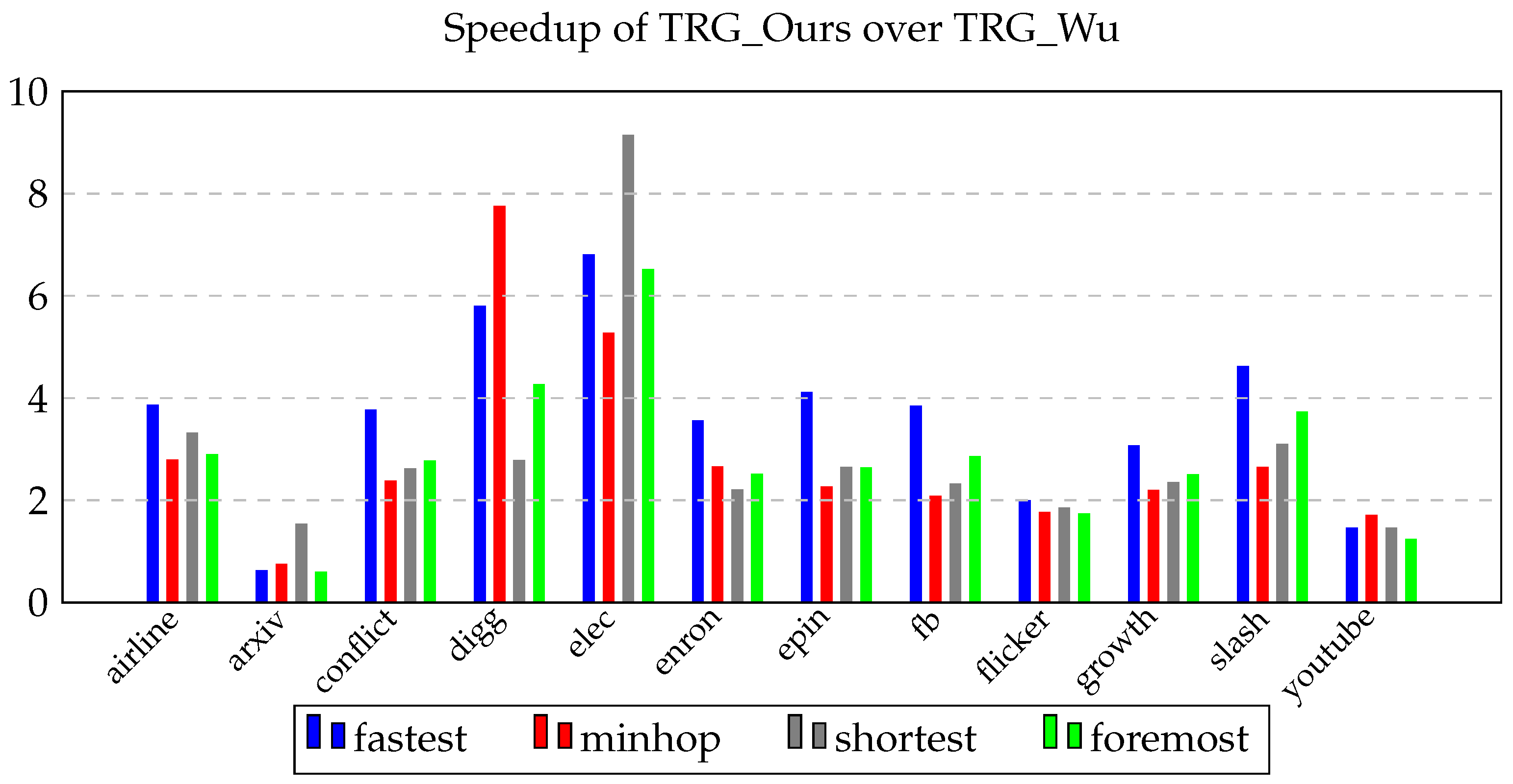
We have developed a new time-respecting graph data structure TRG_Ours for contact sequence temporal graphs. This data structure has fewer vertices and edges than previously proposed TRG structures: TRG_Wu and TRG_Zschoche. Benchmark experiments conducted for the fastest, min-hop, shortest and foremost paths problems indicate that TRG_Ours is superior to TRG_Wu on contact sequence temporal graphs whose TRG is cyclic. In fact, TRG_Ours outperformed TRG_Wu on all but one of our datasets on the fastest paths, min-hop paths, and foremost paths problems. It outperformed TRG_Wu on all 12 datasets for the shortest path problem.

Contact sequence temporal graphs with no edge whose weight is 0 result in acyclic TRGs. For acyclic TRGs, the path problems considered in this paper may be solved more simply using an algorithm based on a topological ordering of the vertices. When there are no edges whose weight is 0, these path problems may be solved using the OSE data structure of [8]. The algorithms for acyclic TRG_Ours were faster than those for acyclic TRG_Wu on all 12 of our datasets and for all four path problems studied in this paper. The acyclic algorithms using TRG_Ours were also faster than the OSE algorithms on all 12 datasets for the fastest paths, min-hop paths, and shortest paths problems but slower on all 12 datasets for the foremost paths problem.

We did not experiment with TRG_Zschoche as this data structure is expected to have more vertices and edges than TRG_Wu (except in the particular case when all edge weights are 1), and so it is expected to give an inferior performance than TRG_Wu. We have also pointed out that TRG structures are superior to OSE on problems requiring only local information (shallow neighborhood search problems), such as one-hop and 2-hop neighbors. So, while Wu et al. [8] conclude that OSE is the data structure of choice for single-source all-destinations problems, our work indicates that TRG structures can be highly competitive with OSE while providing distinct advantages for shallow neighborhood search problems.

References

1. Gheibi, S.; Banerjee, T.; Ranka, S.; Sahni, S. An Effective Data Structure for Contact Sequence Temporal Graphs. In Proceedings of the 2021 IEEE Symposium on Computers and Communications (ISCC), Athens, Greece, 5–8 September 2021; IEEE: Piscataway, NJ, USA, 2021; pp. 1–8. [Google Scholar]
2. Scheideler, C. Models and techniques for communication in dynamic networks. In Proceedings of the Annual Symposium on Theoretical Aspects of Computer Science, Juan les Pins, France, 14–16 March 2002; Springer: Berlin/Heidelberg, Germany, 2002; pp. 27–49. [Google Scholar]
3. Stojmenovic, I. Location updates for efficient routing in ad hoc networks. Handb. Wirel. Netw. Mob. Comput. 2002, 8, 451–471. [Google Scholar]
4. Holme, P.; Saramäki, J. Temporal networks. Phys. Rep. 2012, 519, 97–125. [Google Scholar] [CrossRef]
5. Liu, Y.; Kalagnanam, J.R.; Johnsen, O. Learning dynamic temporal graphs for oil-production equipment monitoring system. In Proceedings of the 15th ACM SIGKDD International Conference on Knowledge Discovery and Data Mining, Paris, France, 28 June–1 July 2009; pp. 1225–1234. [Google Scholar]
6. Bozhenyuk, A.; Belyakov, S.; Knyazeva, M. Modeling objects and processes in gis by fuzzy temporal graphs. In Recent Developments and the New Direction in Soft-Computing Foundations and Applications; Springer: Berlin/Heidelberg, Germany, 2021; pp. 277–286. [Google Scholar]
7. Bui-Xuan, B.M.; Ferreira, A.; Jarry, A. Evolving graphs and least cost journeys in dynamic networks. In Proceedings of the WiOpt’03: Modeling and Optimization in Mobile, Ad Hoc and Wireless Networks, Sophia-Antipolis, France, 3–5 March 2003. 10p. [Google Scholar]
8. Wu, H.; Cheng, J.; Ke, Y.; Huang, S.; Huang, Y.; Wu, H. Efficient algorithms for temporal path computation. IEEE Trans. Knowl. Data Eng. 2016, 28, 2927–2942. [Google Scholar] [CrossRef]
9. Zschoche, P.; Fluschnik, T.; Molter, H.; Niedermeier, R. The complexity of finding small separators in temporal graphs. J. Comput. Syst. Sci. 2020, 107, 72–92. [Google Scholar] [CrossRef]
10. Zhao, A.; Liu, G.; Zheng, B.; Zhao, Y.; Zheng, K. Temporal paths discovery with multiple constraints in attributed dynamic graphs. World Wide Web 2020, 23, 313–336. [Google Scholar] [CrossRef]
11. Ding, P.; Liu, G.; Zhao, P.; Liu, A.; Li, Z.; Zheng, K. Reinforcement Learning Based Monte Carlo Tree Search for Temporal Path Discovery. In Proceedings of the 2019 IEEE International Conference on Data Mining (ICDM), Beijing, China, 8–11 November 2019; IEEE: Piscataway, NJ, USA, 2019; pp. 140–149. [Google Scholar]
12. Hassan, M.S.; Aref, W.G.; Aly, A.M. Graph indexing for shortest-path finding over dynamic sub-graphs. In Proceedings of the Proceedings of the 2016 International Conference on Management of Data, San Francisco, CA, USA, 26 June–1 July 2016; pp. 1183–1197. [Google Scholar]
13. Himmel, A.S.; Bentert, M.; Nichterlein, A.; Niedermeier, R. Efficient computation of optimal temporal walks under waiting-time constraints. In Proceedings of the International Conference on Complex Networks and Their Applications, Lisbon, Portugal, 10–12 December 2019; Springer: Berlin/Heidelberg, Germany, 2019; pp. 494–506. [Google Scholar]
14. Bentert, M.; Himmel, A.S.; Nichterlein, A.; Niedermeier, R. Efficient computation of optimal temporal walks under waiting-time constraints. Appl. Netw. Sci. 2020, 5, 1–26. [Google Scholar] [CrossRef]
15. Casteigts, A.; Himmel, A.S.; Molter, H.; Zschoche, P. Finding temporal paths under waiting time constraints. Algorithmica 2021, 83, 2754–2802. [Google Scholar] [CrossRef]
16. Roditty, L.; Zwick, U. Dynamic approximate all-pairs shortest paths in undirected graphs. Siam J. Comput. 2012, 41, 670–683. [Google Scholar] [CrossRef]
17. Alshammari, M.; Rezgui, A. An all pairs shortest path algorithm for dynamic graphs. Comput. Sci 2020, 15, 347–365. [Google Scholar]
18. Chan, E.P.; Yang, Y. Shortest path tree computation in dynamic graphs. IEEE Trans. Comput. 2008, 58, 541–557. [Google Scholar] [CrossRef]
19. Cicerone, S.; D’Emidio, M.; Frigioni, D. On Mining Distances in Large-Scale Dynamic Graphs. In Proceedings of the ICTCS, Urbino, Italy, 18–20 September 2018; pp. 77–81. [Google Scholar]
20. Hong, J.; Park, K.; Han, Y.; Rasel, M.K.; Vonvou, D.; Lee, Y.K. Disk-based shortest path discovery using distance index over large dynamic graphs. Inf. Sci. 2017, 382, 201–215. [Google Scholar] [CrossRef]
21. Tretyakov, K.; Armas-Cervantes, A.; García-Bañuelos, L.; Vilo, J.; Dumas, M. Fast fully dynamic landmark-based estimation of shortest path distances in very large graphs. In Proceedings of the 20th ACM International Conference on Information and Knowledge Management, Glasgow Scotland, UK, 24–28 October 2011; pp. 1785–1794. [Google Scholar]
22. Wu, H.; Huang, Y.; Cheng, J.; Li, J.; Ke, Y. Reachability and time-based path queries in temporal graphs. In Proceedings of the 2016 IEEE 32nd International Conference on Data Engineering (ICDE), Helsinki, Finland, 16–20 May 2016; IEEE: Piscataway, NJ, USA, 2016; pp. 145–156. [Google Scholar]
23. Dean, B.C. Algorithms for minimum-cost paths in time-dependent networks with waiting policies. Netw. Int. J. 2004, 44, 41–46. [Google Scholar] [CrossRef]
24. Cvetkovski, A.; Crovella, M. Hyperbolic embedding and routing for dynamic graphs. In Proceedings of the IEEE INFOCOM 2009, Rio De Janeiro, Brazil, 19–25 April 2009; IEEE: Piscataway, NJ, USA, 2009; pp. 1647–1655. [Google Scholar]
25. Demetrescu, C.; Italiano, G.F. A new approach to dynamic all pairs shortest paths. J. ACM 2004, 51, 968–992. [Google Scholar] [CrossRef]
26. Clementi, A.; Silvestri, R.; Trevisan, L. Information spreading in dynamic graphs. Distrib. Comput. 2015, 28, 55–73. [Google Scholar] [CrossRef]
27. Zhang, X.; Chan, F.T.; Yang, H.; Deng, Y. An adaptive amoeba algorithm for shortest path tree computation in dynamic graphs. Inf. Sci. 2017, 405, 123–140. [Google Scholar] [CrossRef]
28. Calle, J.; Rivero, J.; Cuadra, D.; Isasi, P. Extending ACO for fast path search in huge graphs and social networks. Expert Syst. Appl. 2017, 86, 292–306. [Google Scholar] [CrossRef]
29. Chen, D.; Navarro-Arribas, G.; Borrell, J. On the applicability of onion routing on predictable delay-tolerant networks. In Proceedings of the 2017 IEEE 42nd Conference on Local Computer Networks (LCN), Singapore, 9 October 2017; IEEE: Piscataway, NJ, USA, 2017; pp. 575–578. [Google Scholar]
30. Fluschnik, T.; Niedermeier, R.; Schubert, C.; Zschoche, P. Multistage st path: Confronting similarity with dissimilarity in temporal graphs. In Proceedings of the 31st International Symposium on Algorithms and Computation (ISAAC 2020), Hong Kong, 14–18 December 2020; Schloss Dagstuhl-Leibniz-Zentrum für Informatik: Wadern, Germany, 2020. [Google Scholar]
31. Chabini, I.; Lan, S. Adaptations of the A* algorithm for the computation of fastest paths in deterministic discrete-time dynamic networks. IEEE Trans. Intell. Transp. Syst. 2002, 3, 60–74. [Google Scholar] [CrossRef]
32. Akrida, E.C.; Mertzios, G.B.; Nikoletseas, S.; Raptopoulos, C.; Spirakis, P.G.; Zamaraev, V. How fast can we reach a target vertex in stochastic temporal graphs? J. Comput. Syst. Sci. 2020, 114, 65–83. [Google Scholar] [CrossRef]
33. Brunelli, F.; Crescenzi, P.; Viennot, L. On Computing Pareto Optimal Paths in Weighted Time-Dependent Networks. Inf. Process. Lett. 2021, 168, 106086. [Google Scholar] [CrossRef]
34. Riazi, S.; Srinivasan, S.; Das, S.K.; Bhowmick, S.; Norris, B. Single-source shortest path tree for big dynamic graphs. In Proceedings of the 2018 IEEE International Conference on Big Data (Big Data), Seattle, WA, USA, 10–13 December 2018; IEEE: Piscataway, NJ, USA, 2018; pp. 4054–4062. [Google Scholar]
35. Ni, P.; Hanai, M.; Tan, W.J.; Wang, C.; Cai, W. Parallel algorithm for single-source earliest-arrival problem in temporal graphs. In Proceedings of the 2017 46th International Conference on Parallel Processing (ICPP), Bristol, UK, 14–17 August 2017; IEEE: Piscataway, NJ, USA, 2017; pp. 493–502. [Google Scholar]
36. Ning, Z.; Dai, G.; Liu, Y.; Ge, Y.; Wu, J. An Improved Index Based on MapReduce for Path Queries in Public Transportation Networks. In Proceedings of the 2018 14th International Conference on Natural Computation, Fuzzy Systems and Knowledge Discovery (ICNC-FSKD), Huangshan, China, 28–30 July 2018; IEEE: Piscataway, NJ, USA, 2018; pp. 919–926. [Google Scholar]
37. Ferone, D.; Festa, P.; Napoletano, A.; Pastore, T. Shortest paths on dynamic graphs: A survey. Pesqui. Oper. 2017, 37, 487–508. [Google Scholar] [CrossRef]
38. Nannicini, G.; Liberti, L. Shortest paths on dynamic graphs. Int. Trans. Oper. Res. 2008, 15, 551–563. [Google Scholar] [CrossRef]
39. Caro, D.; Rodríguez, M.A.; Brisaboa, N.R. Data structures for temporal graphs based on compact sequence representations. Inf. Syst. 2015, 51, 1–26. [Google Scholar] [CrossRef]
Figure 1. Ref. [1] (a) A temporal graph G, (b) OSE(G), (c) TRG_Wu(G), (d) TRG_Zschoche(G), and (e) TRG_Ours(G). For (d,e), as all the nodes belong to sets ϕ ( u ) and V o u t ( u ) , respectively. Therefore, we have not labeled them with the set memberships as we have conducted for (c).
Algorithms 17 00148 g001
Figure 2. Speedup obtained by cyclic TRG_Ours relative to cyclic TRG_Wu.
Algorithms 17 00148 g002
Figure 3. Speedup obtained by our acyclic fastest path algorithm.
Algorithms 17 00148 g003
Figure 4. Speedup obtained by our acyclic min-hop algorithm.
Algorithms 17 00148 g004
Figure 5. Speedup obtained by our acyclic shortest path algorithm.
Algorithms 17 00148 g005
Figure 6. Speedup obtained by our acyclic foremost path algorithm.
Algorithms 17 00148 g006