Efficient Algorithm for Proportional Lumpability and Its Application to Selfish Mining in Public Blockchains

Abstract

This paper explores the concept of proportional lumpability as an extension of the original definition of lumpability, addressing the challenges posed by the state space explosion problem in computing performance indices for large stochastic models. Lumpability traditionally relies on state aggregation techniques and is applicable to Markov chains demonstrating structural regularity. Proportional lumpability extends this idea, proposing that the transition rates of a Markov chain can be modified by certain factors, resulting in a lumpable new Markov chain. This concept facilitates the derivation of precise performance indices for the original process. This paper establishes the well-defined nature of the problem of computing the coarsest proportional lumpability that refines a given initial partition, ensuring a unique solution exists. Additionally, a polynomial time algorithm is introduced to solve this problem, offering valuable insights into both the concept of proportional lumpability and the broader realm of partition refinement techniques. The effectiveness of proportional lumpability is demonstrated through a case study that consists of designing a model to investigate selfish mining behaviors on public blockchains. This research contributes to a better understanding of efficient approaches for handling large stochastic models and highlights the practical applicability of proportional lumpability in deriving exact performance indices.

1. Introduction

Markov chains serve as the fundamental semantic model for a multitude of modeling formalisms employed in the reliability analysis and performance evaluation of complex systems, including Stochastic Petri nets [1,2], Stochastic Automata Networks [3,4], queuing networks [5,6], and Markovian process algebras [7,8].

Although the utilization of high-level specification formalisms greatly simplifies the creation of compositional and hierarchical quantitative models, even seemingly straightforward models can pose challenges due to a large number of states, making analysis a daunting task. To tackle this problem, exploring models with extensive state spaces without resorting to approximation or simulation techniques involves reducing the state space of the underlying Markov chain by aggregating states that exhibit equivalent behaviors [9,10]. This state-based reduction technique is known as lumping. Various notions of lumping, including strong and weak lumping [11], exact lumping [9,12], and strict lumping [13], have been introduced in the literature. The lumpability method enables efficient computation of exact performance indices [14] when the model is lumpable.

It is widely recognized that not all Markov chains are inherently lumpable, particularly those originating from real-world applications. To overcome this limitation, the notion of quasi-lumpability was introduced in [15], suggesting that transforming a quasi-lumpable Markov chain into a lumpable one allows for the application of steady state probability bounding methods [15,16,17,18,19] to obtain bounds on the performance indices of the original model.

In [20], the concept of proportional lumpability was introduced, expanding upon the original notion of lumpability. Unlike the broader definition of quasi-lumpability, proportional lumpability allows for the derivation of precise performance indices for the original process. Building on this foundation, our research in [21] delves deeper into the topic by juxtaposing proportional lumpability with other lumping definitions, such as weak lumpability [11,22], and the concept of exact lumpability for ordinary differential equations (ODEs) [23,24].

The definition of proportional lumpability entails identifying a function that assigns a positive coefficient to each state of the system. However, given the infinite set of potential functions, devising an efficient algorithmic technique to check or compute proportional lumpability is not immediately evident.

This paper explores the properties of proportional lumpability and elaborates on three alternative characterizations. The first, proven in [21], enables efficient verification of whether a partition of the state space is induced by an equivalence relation representing proportional lumpability. The second, proven in [25], is used to design an algorithm to calculate the coarsest proportional lumpability of a given Markov chain in time $O\left(\right|\mathcal{S}{|}^4)$ with $\left|\mathcal{S}\right|$ being the cardinality of the state space of the analyzed model. The third characterization is a novel contribution, and it allows us to improve on the above complexity by obtaining an algorithm for proportional lumpability running in $O\left(\right|\mathcal{S}{|}^{2}log\left|\mathcal{S}\right|)$. Similar to partition refinement algorithms used for the traditional concept of strong (or ordinary) lumpability, our approach demonstrates that computing the coarsest proportional lumpability refining a given initial partition is well defined, always yielding a unique solution. Furthermore, we demonstrate that the maximum proportional lumpability over an initial Markov chain, within a specified equivalence relation, can be interpreted as ordinary lumpability over a perturbation of the original chain. Consequently, we can leverage efficient algorithms for calculating the maximum lumpability over a Markov chain.

The effectiveness of proportional lumpability is illustrated through the presentation of a comprehensive case study. This study involves the development and analysis of a proportionally lumpable model specifically tailored for examining selfish mining behaviors within a public blockchain context. Our aim is to provide valuable insights into the concept of proportional lumpability and the broader applications of partition refinement techniques.

This work extends our prior investigations outlined in [25,26]. Expanding upon our earlier research on proportional lumpability [25], we introduce a pivotal, novel, third characterization in this paper. This result allows us to enhance the efficiency of our previously proposed algorithm, resulting in a groundbreaking approach to proportional lumpability. The algorithm now boasts a remarkable time complexity of $O\left(\right|\mathcal{S}{|}^{2}log\left|\mathcal{S}\right|)$, where $\left|\mathcal{S}\right|$ denotes the cardinality of the state space of the analyzed model, offering the potential to substantially enhance the scalability and applicability of proportional lumpability analyses. Furthermore, we expand on the findings in [25] by offering a thorough case study. This study is inspired by our previous work [26], where a strongly lumpable model for a concrete blockchain problem was presented. The model is carefully designed to investigate selfish mining behaviors within the framework of a public blockchain. In this paper, we present an extended version of the model studied in [26], designed to capture a more realistic configuration of the blockchain state under examination. Our analysis reveals that despite this broadening, the generalized model maintains its computational manageability. This resilience primarily stems from its adherence to a more general definition of lumpability, specifically, proportionally lumpability. Consequently, we can apply the findings presented in this paper to conduct precise analyses of the new model. This comprehensive approach aims to shed light on the dynamics of selfish mining in the real-world context of blockchain technology.

The structure of this paper is as follows: In Section 2, we delve into the theoretical underpinnings of continuous-time Markov chains and revisit the concept of strong (or ordinary) lumpability. Section 3 introduces the notion of proportional lumpability, providing a novel characterization of it along with an efficient algorithm for its verification. We discuss both the accuracy and complexity of the algorithm. In Section 4, we present a case study centered around a proportionally lumpable model for selfish mining in public blockchain. Finally, Section 5 offers concluding remarks and future directions to wrap up the paper.

2. Background

In this section, we provide a brief overview of the basics of continuous-time Markov chains [11,27,28] and introduce the notion of lumpability [22,29,30].

2.1. Stochastic Models

In this paper, we consider Markov chains or Markov processes that are stochastic models describing sequences of possible events in which the probability of each event depends only on the state attained in the previous event. More specifically, we concentrate on Continuous-Time Markov Chains.

A Continuous-Time Markov Chain (CTMC) with finite or countable state space $\mathcal{S}$ is a family $\left\{X\left(t\right)\right|t\in {\mathbb{R}}^{+}\}$ of $\mathcal{S}$-valued random variables such that

$$\begin{array}{cc}\mathit{Prob}(X\left(t_{n+1}\right)=s_{n+1}|X\left(t_1\right)=s_1,X\left(t_2\right)=s_2,\dots ,\hfill & X\left(t_n\right)=s_n)=\hfill \\ & \hfill \mathit{Prob}(X\left(t_{n+1}\right)=s_{n+1}|X\left(t_n\right)=s_n).\end{array}$$

This condition is the natural continuous-time analogue of the Markov property. It requires that the future behavior of the process is conditionally independent of its past evolution given the present states.

We assume that the Markov properties under consideration satisfy the following properties: a Markov process $X\left(t\right)$ is

• stationary if its statistical properties do not change by time, i.e., the family of random variables $(X\left(t_1\right),X\left(t_2\right),\dots ,X\left(t_n\right))$ has the same distribution as the collection $(X(t_1+\tau ),X(t_2+\tau ),\dots ,X(t_n+\tau ))$ for all $t_1,t_2,\dots ,t_n,\tau \in {\mathbb{R}}^{+}$.
• time-homogeneous if the conditional probability $\mathit{Prob}(X(t+\tau )=s|X\left(t\right)=s^{\prime })$ remains constant regardless of t, i.e., the behavior of the system does not depend on when it is observed. In particular, the transitions between states are independent of the time at which the transitions occur.
• irreducible if all states in its state space $\mathcal{S}$ can be reached from all other states by following the transitions of the process.

Within a Markov process, a state is labeled persistent or recurrent if the probability of the process eventually returning to that state is one. Otherwise, the state is called transient. In terms of a system, the recurrent states correspond to the behavior which is repeatedly exhibited by the system, whereas transient states correspond to a behavior which will be no longer exhibited after a certain time. A recurrent state is termed positive-recurrent or ergodic if the expected number of steps until the process returns to that state is less than infinity. A Markov process is ergodic if all its states are positive-recurrent. In the context of finite Markov chains, irreducibility alone ensures ergodicity. In this paper, we consider Continuous-Time Markov Chains, which are time-homogeneous, irreducible, and ergodic.

An ergodic Continuous-Time Markov Chain (CTMC) possesses an equilibrium (or steady-state) distribution, defined as the unique collection of positive real numbers $\pi \left(s\right)$ where $s\in \mathcal{S}$, satisfying the equation:

$$\underset{t\to \infty }{lim}\mathit{Prob}(X\left(t\right)=s|X\left(0\right)=s^{\prime })=\pi \left(s\right).$$

It is worth noting that the above equation for $\pi \left(s\right)$ is independent of $s^{\prime }$. We denote by $q(s,s^{\prime })$ the transition rate from state s to state $s^{\prime }$, where $s\ne s^{\prime }$. The sum of all transition rates out of state s to any other state in the chain is denoted as $q\left(s\right)$. A state s for which $q\left(s\right)=\infty$ is termed an instantaneous state, as it is instantaneously left upon entry. While theoretically possible, we assume throughout that $0<q\left(s\right)<\infty$ for each state s.

The infinitesimal generator matrix $\mathbf{Q}$ of a CTMC $X\left(t\right)$ with state space $\mathcal{S}$ is defined as the $\left|\mathcal{S}\right|\times \left|\mathcal{S}\right|$ matrix. Its off-diagonal elements are the $q(s,s^{\prime })$’s, and its diagonal elements are the negative sum of the off-diagonal elements of each row, i.e., $q(s,s)=-{\sum }_{s^{\prime }\in \mathcal{S},s^{\prime }\ne s}q(s,s^{\prime })$. For simplicity, we use $q(s,s^{\prime })$ to denote the components of matrix $\mathbf{Q}$. For $s\in \mathcal{S}$ and $S\subseteq \mathcal{S}$, we write $q(s,S)$ to denote ${\sum }_{s^{\prime }\in S}q(s,s^{\prime })$.

Any non-trivial vector of positive real numbers $\mathit{\mu }$ satisfying the system of global balance equations (GBEs) $\mathit{\mu }\mathbf{Q}=\mathbf{0}$ is referred to as an invariant measure of the CTMC.

Given an irreducible CTMC $X\left(t\right)$, if ${\mathit{\mu }}_1$ and ${\mathit{\mu }}_2$ are two invariant measures of $X\left(t\right)$, then there exists a constant $k>0$ such that ${\mathit{\mu }}_1=k{\mathit{\mu }}_2$. If the CTMC is ergodic, then there exists a unique invariant measure $\mathit{\pi }$ whose components sum to unity, i.e., ${\sum }_{s\in \mathcal{S}}\pi \left(s\right)=1$. In this case, $\mathit{\pi }$ represents the equilibrium or steady-state distribution of the CTMC.

2.2. Strong (or Ordinary) Lumpability

In the field of performance and reliability analysis, the notion of lumpability introduces a method for aggregating models. This method allows for the development of a reduced Markov chain compared to the original one while maintaining the ability to determine precise results for the original process.

The concept of lumpability is defined by equivalence relations that span the state space of the Markov chain. These relations create a division within the state space of the Markov chain, enabling the grouping of equivalent states into larger macro-states, which ultimately decreases the total state space. When the division fulfills the strong (or ordinary) lumpability condition [11,31], the equilibrium solution of the condensed process can provide a precise solution for the initial one.

The definition of strong lumpability was originally presented in [11] and has been extensively investigated in subsequent research [13,24,32,33,34].

Definition 1 

(Strong lumpability). Consider a CTMC $X\left(t\right)$ with a state space $\mathcal{S}$, and let ∼ denote an equivalence relation over $\mathcal{S}$. We define $X\left(t\right)$ to be strongly lumpable with respect to ∼ (or, alternatively, ∼ is termed as trong lumpability for $X\left(t\right)$) if ∼ induces a partition on the state space of $X\left(t\right)$ such that for any equivalence classes $S_i,S_j\in \mathcal{S}/\sim$ where $S_i\ne S_j$, and for any states $s,s^{\prime }\in S_i$, the transition rates from s to $S_j$ and from $s^{\prime }$ to $S_j$ are equal, i.e.,

$$q(s,S_j)=q(s^{\prime },S_j).$$

Therefore, an equivalence relation over the state space of a Markov process has a strong lumpability if it divides the space into equivalence classes, ensuring that within each class, the collective transition rates to any other class remain the same. It is important to highlight that every Markov process exhibits strong lumpability with respect to the identity relation, as well as the trivial relation, which comprises only one equivalence class.

In the paper by Kemeny et al. [11], it is demonstrated that for an equivalence relation ∼ over the state space of a Markov process $X\left(t\right)$, the aggregated process remains a Markov process for any initial distribution if and only if ∼ represents a strong lumpability for $X\left(t\right)$. Furthermore, the transition rate between two macro-states $S_i$ and $S_j$ in $\mathcal{S}/\sim$ is equal to $q(s,S_j)$ for any s belonging to $S_i$.

Proposition 1 

(Aggregated process for strong lumpability). Consider a CTMC $X\left(t\right)$ with a state space $\mathcal{S}$, infinitesimal generator $\mathbf{Q}$, and equilibrium distribution π. Let ∼ be a strong lumpability for $X\left(t\right)$ and $\tilde{X}\left(t\right)$ be the aggregated process with state space $\mathcal{S}/\sim$ and infinitesimal generator $\tilde{\mathbf{Q}}$ defined by, for any equivalence class $S_i,S_j\in \mathcal{S}/\sim$,

$$\tilde{q}(S_i,S_j)=q(s,S_j)$$

for any $s\in S_i$. Then, the equilibrium distribution $\tilde{\mathit{\pi }}$ of $\tilde{X}\left(t\right)$ is characterized by the property that for any equivalence class $S\in \mathcal{S}/\sim$,

$$\tilde{\pi }\left(S\right)=\sum _{s\in S}\pi \left(s\right).$$

3. Proportional Lumpability

The notion of proportional lumpability made its debut in [20]. Much like the notion of quasi-lumpability [15], which is also known as near-lumpability in [13], proportional lumpability builds upon the initial concept of strong lumpability. Furthermore, in contrast to the broader scope of quasi-lumpability, proportional lumpability allows for the precise derivation of a solution for the original process.

Definition 2 

(Proportional lumpability). Consider a CTMC $X\left(t\right)$ with a state space $\mathcal{S}$, and let ∼ denote an equivalence relation over $\mathcal{S}$. We define $X\left(t\right)$ to be proportionally lumpable with respect to ∼ (or, alternatively, ∼ is termed a proportional lumpability for $X\left(t\right)$) if ∼ induces a partition on the state space of $X\left(t\right)$ such that for any equivalence classes $S_i,S_j\in \mathcal{S}/\sim$ where $S_i\ne S_j$, and for any states $s,s^{\prime }\in S_i$,

$$\frac{q(s,S_j)}{\kappa \left(s\right)}=\frac{q(s^{\prime },S_j)}{\kappa \left(s^{\prime }\right)}.$$

where κ is a function from $\mathcal{S}$ to ${\mathbb{R}}^{+}$. We say that $X\left(t\right)$ is κ-proportionally lumpable with respect to ∼ (or, alternatively, ∼ is a κ-proportional lumpability for $X\left(t\right)$) if $X\left(t\right)$ is proportionally lumpable with respect to ∼ and function κ.

The next theorem proven in [20] establishes that proportional lumpability facilitates the calculation of a precise solution for the original model.

Theorem 1 

(Aggregated process for proportional lumpability). Consider a CTMC $X\left(t\right)$ with a state space $\mathcal{S}$, infinitesimal generator $\mathbf{Q}$, and equilibrium distribution π. Let κ denote a function from $\mathcal{S}$ to ${\mathbb{R}}^{+}$, ∼ be a κ-proportional lumpability for $X\left(t\right)$, and $\tilde{X}\left(t\right)$ be the aggregated process over the state space $\mathcal{S}/\sim$ and with infinitesimal generator $\tilde{\mathbf{Q}}$ defined by, for any equivalence classes $S_i,S_j\in \mathcal{S}/\sim$ where $S_i\ne S_j$, and for any state $s,\in S_i$,

$$\tilde{q}(S_i,S_j)=\frac{q(s,S_j)}{\kappa \left(s\right)}.$$

Then, $\tilde{\mathit{\mu }}$ such that for any equivalence class $S\in \mathcal{S}/\sim$,

$$\tilde{\mu }\left(S\right)=\sum _{s\in S}\pi \left(s\right)\kappa \left(s\right)$$

(1)

is an invariant measure of $\tilde{X}\left(t\right)$.

Definition 3 elucidates a technique for perturbing a CTMC that is proportionally lumpable, transforming it into one that is strongly lumpable. Unlike earlier perturbation approaches, Theorem 2 furnishes a method to calculate the stationary probabilities of a proportionally lumpable chain by leveraging those of the perturbed lumpable chain. The proof of Theorem 2 is available in [20].

Definition 3 

(Perturbed Markov chains). Consider a CTMC $X\left(t\right)$ with a state space $\mathcal{S}$ and infinitesimal generator $\mathbf{Q}$. Let κ denote a function from $\mathcal{S}$ to ${\mathbb{R}}^{+}$. We say that a CTMC $X^{\prime }\left(t\right)$ with infinitesimal generator ${\mathbf{Q}}^{\prime }$ is a perturbation of $X\left(t\right)$ with respect to κ if $X^{\prime }\left(t\right)$ is obtained from $X\left(t\right)$ by perturbing its rates such that for all $s,s^{\prime }\in \mathcal{S}$ with $s\ne s^{\prime }$,

$$q^{\prime }(s,s^{\prime })=\frac{q(s,s^{\prime })}{\kappa \left(s\right)}.$$

Theorem 2 

(Equilibrium distribution for proportional lumpability). Let $X\left(t\right)$ be a CTMC with state space $\mathcal{S}$, infinitesimal generator $\mathbf{Q}$, and equilibrium distribution π. Let κ be a function from $\mathcal{S}$ to ${\mathbb{R}}^{+}$. For any perturbation $X^{\prime }\left(t\right)$ of the original chain $X\left(t\right)$ with respect to κ, as per Definition 3, where $X^{\prime }\left(t\right)$ has an infinitesimal generator ${\mathbf{Q}}^{\prime }$ and equilibrium distribution ${\mathit{\pi }}^{\prime }$, the equilibrium distribution π of $X\left(t\right)$ adheres to the following property: let $K={\sum }_{s\in \mathcal{S}}{\pi }^{\prime }\left(s\right)/\kappa \left(s\right)$, then for all $s\in \mathcal{S}$,

$$\pi \left(s\right)=\frac{{\pi }^{\prime }\left(s\right)}{K\kappa \left(s\right)}.$$

Example 1. 

Consider the classic reliability problem concerning a system comprising N components. Each component $i\in 1,\dots ,N$ follows an exponential distribution with rate ${\mu }_i$ for time to failure, independent of the other components. This system type has been extensively researched, as seen in various works such as [35,36,37,38,39]. Following the approach in [38], we posit that upon system failure, it is restored to a new “good” state, and the restoration time follows an exponential distribution with rate λ. At any given time, the system state can be represented as a boolean vector of size N, $\overline{x}=(x_1,\dots ,x_N)$, where $x_i=1$ signifies the i-th component functioning and $x_i=0$ denotes failure. Consequently, the set of all feasible states is $\mathcal{S}={\{0,1\}}^N$. Under these conditions, the system’s state evolution over time can be modeled by a continuous-time Markov chain. The Markov process for a system with 3 components (i.e., $N=3$) is illustrated in Figure 1. Notably, this system is proportionally lumpable with respect to the given partition: $S_n=\{\overline{x}\in \mathcal{S}:\sum x_i=n\}$ with $n\in \{0,1,2,3\}$, i.e.,

• $\begin{array}{ccc}{S}_0\hfill & =& \left\{\right(0,0,0\left)\right\}\hfill \\ S_1\hfill & =& \left\{\right(1,0,0),(0,1,0),(0,0,1\left)\right\}\hfill \\ S_2\hfill & =& \left\{\right(1,1,0),(1,0,1),(0,1,1\left)\right\}\hfill \\ S_3\hfill & =& \left\{\right(1,1,1\left)\right\}\hfill \end{array}$

and the function κ such that for each state $s\in S_1\cup S_2$, $\kappa \left(s\right)=q\left(s\right)$, while for $s\in S_0\cup S_3$, $\kappa \left(s\right)=1$. Consequently, we can examine the aggregated Markov chain depicted in Figure 2. Utilizing Theorems 1 and 2, we are able to calculate the precise solution for the original model.

3.1. Three Alternative Characterizations of Proportional Lumpability

We introduce three alternative characterizations of proportional lumpability. The first one, proven in [21], provides an efficient method to determine if a partition of a Markov chain’s state space is induced by proportional lumpability. The second characterization, outlined in [25], has been utilized to describe an algorithm for computing the coarsest proportional lumpability of a given Markov chain in $O\left(\right|\mathcal{S}{|}^4)$ time. The third characterization is new, and it allows us to improve on the above complexity of obtaining an algorithm running in $O\left(\right|\mathcal{S}{|}^{2}log\left|\mathcal{S}\right|)$.

First, for a given equivalence relation ∼ over the state space of a CTMC, we denote by $q_{\sim }\left(s\right)$ the sum of all transition rates from the state s to any state t such that $s\nsim t$, i.e., for all $s\in \mathcal{S}$,

$$q_{\sim }\left(s\right)=\sum _{t\nsim s}q(s,t).$$

The following theorem shows that proportional lumpability can be characterized in terms of $q_{\sim }\left(s\right)$ by replacing $\kappa \left(s\right)$ with $q_{\sim }\left(s\right)$ in the original definition.

Theorem 3 

(Characterization 1 of proportional lumpability [21]). Let $X\left(t\right)$ be an ergodic CTMC with state space $\mathcal{S}$ and ∼ be an equivalence relation over $\mathcal{S}$. The relation ∼ is a proportional lumpability for $X\left(t\right)$ if and only if for any equivalence classes $S_i,S_j\in \mathcal{S}/\sim$ with $S_i\ne S_j$ and $s,s^{\prime }\in S_i$,

• $q_{\sim }\left(s\right)\ne 0$ if and only if $q_{\sim }\left(s^{\prime }\right)\ne 0$
• if $q_{\sim }\left(s\right)\ne 0$ then

  $$\frac{q(s,S_j)}{q_{\sim }\left(s\right)}=\frac{q(s^{\prime },S_j)}{q_{\sim }\left(s^{\prime }\right)}.$$

While the aforementioned characterization is useful for efficiently verifying whether a given relation conforms to proportional lumpability, its direct application in an algorithm for computing proportional lumpability refinement from an initial relation is not immediately apparent. As we will demonstrate below, if the relation undergoes changes during computation, $q_{\sim }$ also changes. Consequently, an equality from item 2 that is false in the current step might become true later. Conversely, the following characterization of proportional lumpability is more straightforward to employ in defining a partition refinement algorithm for proportional lumpability.

Theorem 4 

(Characterization 2 of proportional lumpability [25]). Consider a CTMC $X\left(t\right)$ with a state space $\mathcal{S}$, and let ∼ denote an equivalence relation over $\mathcal{S}$. The relation ∼ is a proportional lumpability for $X\left(t\right)$ if and only if for any equivalence classes $S_i,S_j,S_k\in \mathcal{S}/\sim$ where $S_i\ne S_j$, $S_i\ne S_k$, and $s,s^{\prime }\in S_i$,

• $q(s,S_k)\ne 0$ if and only if $q(s^{\prime },S_k)\ne 0$ and
• if $q(s,S_k)\ne 0$, then

  $$\frac{q(s,S_j)}{q(s,S_k)}=\frac{q(s^{\prime },S_j)}{q(s^{\prime },S_k)}$$

In order to introduce our new characterization, we need to recall that, as for strong lumpability, also in the case of proportional lumpability the equivalence relation $\mathcal{S}\times \mathcal{S}$ is always a proportional lumpability. However, this is not useful in the applications. On the other hand, the problem of “refining” a given initial equivalence relation in order to obtain a proportional lumpability is a challenging one.

Definition 4 

(Maximum Proportional Lumpability Problem). Let $X\left(t\right)$ be a CTMC with state space $\mathcal{S}$ and let $\mathcal{R}$ be an equivalence relation over $\mathcal{S}$. The maximum proportional lumpability problem over $X\left(t\right)$ and $\mathcal{R}$ consists of finding the largest equivalence relation ∼ such that $\sim \subseteq \mathcal{R}$ and ∼ is a proportional lumpability for $X\left(t\right)$.

In [25], we proved that the maximum proportional lumpability problem has always a unique solution that can be computed in time $O\left(\right|\mathcal{S}{|}^4)$. The following characterization allows us to improve such time complexity result. We recall that given an equivalence relation $\mathcal{R}$, $q_{\mathcal{R}}\left(s\right)$ denotes the sum of all transition rates from s to any state t such that $(s,t)\notin \mathcal{R}$. Notice that in Theorem 3, we referred to a generic equivalence relation ∼; hence, since we consider only ergodic CTMCs, the first item is only necessary to cover the case in which the relation ∼ is the total relation $\mathcal{S}\times \mathcal{S}$. In the following result, we do not have to explicitly deal with it, since we consider an equivalence relation $\mathcal{R}$ which is not total.

Theorem 5 

(Characterization 3 of proportional lumpability). Let $X\left(t\right)$ be an ergodic CTMC with state space $\mathcal{S}$ and $\mathcal{R}$ be an equivalence relation over $\mathcal{S}$ with $\mathcal{R}\ne \mathcal{S}\times \mathcal{S}$. The relation ∼ is the maximum proportional lumpability over $X\left(t\right)$ and $\mathcal{R}$ if and only if it is the largest equivalence relation included in $\mathcal{R}$ such that for any equivalence classes $S_i,S_j\in \mathcal{S}/\sim$ with $S_i\ne S_j$ and $s,s^{\prime }\in S_i$,

$$\frac{q(s,S_j)}{q_{\mathcal{R}}\left(s\right)}=\frac{q(s^{\prime },S_j)}{q_{\mathcal{R}}\left(s^{\prime }\right)}$$

Proof. 

$\Rightarrow )$ Suppose that ∼ is the maximum proportional lumpability over $X\left(t\right)$ and $\mathcal{R}$. This means that ∼ is the largest equivalence relation included in $\mathcal{R}$ for which there exists a function $\kappa$ from $\mathcal{S}$ to ${\mathbb{R}}^{+}$ such that ∼ is a $\kappa$-proportional lumpability. This means that ∼ is such that for any equivalence classes $S_i,S_j\in \mathcal{S}/\sim$ with $S_i\ne S_j$ and $s,s^{\prime }\in S_i$

$$\frac{q(s,S_j)}{\kappa \left(s\right)}=\frac{q(s^{\prime },S_j)}{\kappa \left(s^{\prime }\right)}$$

Let B be a union of equivalence classes of ∼. It holds that $q(s,B)\ne 0$ if and only if $q(s^{\prime },B)\ne 0$. Moreover,

$$\frac{q(s,B)}{\kappa \left(s\right)}=\frac{q(s^{\prime },B)}{\kappa \left(s^{\prime }\right)}$$

If $q(s,B)\ne 0$, this is equivalent to

$$\frac{\kappa \left(s\right)}{q(s,B)}=\frac{\kappa \left(s^{\prime }\right)}{q(s^{\prime },B)}$$

As a consequence,

$$\frac{q(s,S_j)}{q(s,B)}=\frac{q(s,S_j)}{\kappa \left(s\right)}\frac{\kappa \left(s\right)}{q(s,B)}=\frac{q(s^{\prime },S_j)}{\kappa \left(s^{\prime }\right)}\frac{\kappa \left(s^{\prime }\right)}{q(s^{\prime },B)}=\frac{q(s^{\prime },S_j)}{q(s^{\prime },B)}$$

Let $B_i$ be the equivalence class of $\mathcal{R}$ to which s and $s^{\prime }$ belong. It holds that $S_i\subseteq B_i$. Moreover, $\mathcal{S}\setminus B_i$ is a union of equivalence classes of ∼. Since $X\left(t\right)$ is ergodic, $\mathcal{R}\ne \mathcal{S}\times \mathcal{S}$, and $s\sim s^{\prime }$, it has to be $q(s,\mathcal{S}\setminus B_i)=q_{\mathcal{R}}\left(s\right)\ne 0$ and $q(s^{\prime },\mathcal{S}\setminus B_i)=q_{\mathcal{R}}\left(s\right)\ne 0$. Hence, ∼ satisfies

$$\frac{q(s,S_j)}{q_{\mathcal{R}}\left(s\right)}=\frac{q(s^{\prime },S_j)}{q_{\mathcal{R}}\left(s^{\prime }\right)}$$

Finally, ∼ has to be the largest equivalence relation included in $\mathcal{R}$ that satisfies such equations, since any equivalence relation included in $\mathcal{R}$ satisfying such equations is a proportional lumpability and ∼ is by hypothesis the largest proportional lumpability included in $\mathcal{R}$.

⇐) Suppose that ∼ is the largest equivalence relation included in $\mathcal{R}$ that satisfies the equations

$$\frac{q(s,S_j)}{q_{\mathcal{R}}\left(s\right)}=\frac{q(s^{\prime },S_j)}{q_{\mathcal{R}}\left(s^{\prime }\right)}$$

Since $\mathcal{R}\ne \mathcal{S}\times \mathcal{S}$ and $X\left(t\right)$ is ergodic, it holds that $q_{\mathcal{R}}\left(s\right)$ is greater than 0 for each $s\in \mathcal{S}$. Hence, ∼ is a proportional lumpability included in $\mathcal{R}$. We still have to prove that it is the largest one. Let us assume by contraddiction that there exists another proportional lumpability ≈ included in $\mathcal{R}$ and larger than ∼. There exists a function $\kappa$ from $\mathcal{S}$ to ${\mathcal{R}}^{+}$ such that ≈ is a $\kappa$-proportional lumpability. This means that for any equivalence classes $T_i,T_j\in \mathcal{S}/\approx$ with $T_i\ne T_j$ and $s,s^{\prime }\in T_i$,

$$\frac{q(s,T_j)}{\kappa \left(s\right)}=\frac{q(s^{\prime },T_j)}{\kappa \left(s^{\prime }\right)}$$

As a consequence, if B is a union of equivalence classes of ≈, it holds that

$$\frac{q(s,B)}{\kappa \left(s\right)}=\frac{q(s^{\prime },B)}{\kappa \left(s^{\prime }\right)}$$

Hence, if $q(s,B)\ne 0$,

$$\frac{\kappa \left(s\right)}{q(s,B)}=\frac{\kappa \left(s^{\prime }\right)}{q(s^{\prime },B)}$$

Let $B_i$ be the equivalence class of $\mathcal{R}$ to which s and $s^{\prime }$ belong. The set $\mathcal{S}\setminus B_i$ is a union of equivalence classes of ≈. Therefore ≈ also satisfies

$$\frac{q(s,T_j)}{q_{\mathcal{R}}\left(s\right)}=\frac{q(s^{\prime },T_j)}{q_{\mathcal{R}}\left(s^{\prime }\right)}$$

which contradicts the fact that ∼ was the largest satisfying such equations.    □

As a consequence, the maximum proportional lumpability over a CTMC $X\left(t\right)$ included in a given equivalence relation $\mathcal{R}$ can be seen as a lumpability over the perturbed chain $X^{\prime }\left(t\right)$ in which the rate $q(s,s^{\prime })$ is divided by $q_{\mathcal{R}}\left(s\right)$.

Corollary 1. 

Let $X\left(t\right)$ be an ergodic CTMC with state space $\mathcal{S}$ and let $\mathcal{R}$ be an equivalence relation over $\mathcal{S}$ with $\mathcal{R}\ne \mathcal{S}\times \mathcal{S}$. The relation ∼ is the maximum proportional lumpability over $X\left(t\right)$ and $\mathcal{R}$ if and only if it is the largest lumpability included in $\mathcal{R}$ over the CTMC $X_{\mathcal{R}}\left(t\right)$ whose infinitesimal generator ${\mathbf{Q}}_{\mathcal{R}}$ is defined as

$$q_{\mathcal{R}}(s,s^{\prime })=\frac{q(s,s^{\prime })}{q_{\mathcal{R}}\left(s\right)}$$

Hence, we can exploit any efficient algorithm for computing the maximum lumpability included in a given equivalence relation in order to compute the maximum proportional lumpability included in the same equivalence relation, as illustrated in Algorithm 1.

Algorithm 1 Computation of the Maximum Proportional Partition

1: function  MaxProp($\mathcal{S},\mathbf{Q},\mathcal{R}$)   2:        if $\mathcal{R}=\mathcal{S}\times \mathcal{S}$ then return $\mathcal{R}$   3:        for $s\in \mathcal{S}$ do   4:               $q_{\mathcal{R}}\left(s\right)=0$   5:               for $s^{\prime }\in \mathcal{S}$ do   6:                  if $(s,s^{\prime })\notin \mathcal{R}$ then   7:                      $q_{\mathcal{R}}\left(s\right)=q_{\mathcal{R}}\left(s\right)+q(s,s^{\prime })$   8:        for $s\in \mathcal{S}$ do   9:               for $s^{\prime }\in \mathcal{S}$ do 10:                  $q_{\mathcal{R}}(s,s^{\prime })=q(s,s^{\prime })/q_{\mathcal{R}}\left(s\right)$ 11:       return MaxLump(${\mathbf{Q}}_{\mathcal{R}}$,$\mathcal{R}$)

The correctness of the described algorithm is immediately followed by Corollary 1, while its complexity depends on the complexity of the subroutine used for computing the maximum lumpability.

Corollary 2 

(Correctness and Complexity). Let MaxLump be an algorithm that, given the infinitesimal generator ${\mathbf{Q}}^{\prime }$ of a CTMC $X^{\prime }\left(t\right)$ and an equivalence relation $\mathcal{R}$ over the states of the chain, computes the largest lumpability of $X^{\prime }\left(t\right)$ included in $\mathcal{R}$. Let $\mathbf{Q}$ be the infinitesimal generator of a CTMC $X\left(t\right)$ over state space $\mathcal{S}$ and $\mathcal{R}$ be an equivalence relation over $\mathcal{S}$. It holds that MaxProp($\mathcal{S},\mathbf{Q},\mathcal{R}$) returns the largest proportional lumpability of $X\left(t\right)$ included in $\mathcal{R}$. Moreover MaxProp has the same time complexity as MaxLump.

Currently, the fastest algorithm for computing the largest lumpability runs in time $O\left(\right|\mathcal{S}{|}^{2}log\left|\mathcal{S}\right|)$ if the infinitesimal generator of the chain is provided as a matrix [40,41].

3.2. Comparison with Lumpability of the Embedded Markov Chain

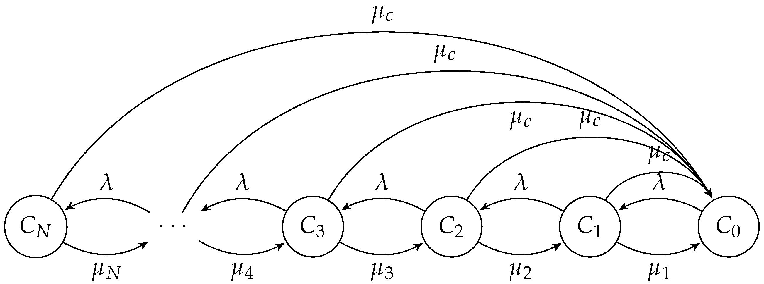
We contrast proportional lumpability with the lumpability of the embedded Markov chain, as defined in [21]. Examples 2 and 3 offer fresh insights into this comparison.

One common method for determining the stationary probability distribution of an ergodic continuous-time Markov chain $X\left(t\right)$ involves examining its embedded Markov chain $X^E\left(t\right)$. Technically, the embedded Markov chain is a regular discrete-time Markov chain (DTMC), sometimes referred to as its jump process. For a given $X\left(t\right)$ with state space $\mathcal{S}$, each entry of the one-step transition probability matrix of the corresponding embedded Markov chain is denoted by $p(s,s^{\prime })$, signifying the conditional probability of transitioning from state s to state $s^{\prime }$. This probability is defined as follows:

$$p(s,s^{\prime })=\frac{q(s,s^{\prime })}{q\left(s\right)}fors\ne s^{\prime }$$

while $p(s,s)=0$. Let us assume that $X^E\left(t\right)$ is aperiodic, and let ${\mathit{\pi }}^{*}$ be its steady-state distribution. Therefore, we can compute the equilibrium distribution $\mathit{\pi }$ of $X\left(t\right)$ in the following way: let $W={\sum }_{s\in \mathcal{S}}{\pi }^{*}\left(s\right)/q\left(s\right)$, then

$$\pi \left(s\right)=\frac{{\pi }^{*}\left(s\right)}{Wq\left(s\right)}.$$

It is important to note that our definition of $q_{\sim }\left(s\right)$ differs from that of $q\left(s\right)$ in general. Therefore, the proportionally lumpable property of $X\left(t\right)$ does not necessarily imply that the corresponding embedded Markov chain $X^E\left(t\right)$ is lumpable. Conversely, if $X^E\left(t\right)$ exhibits lumpability, then $X\left(t\right)$ is proportionally lumpable with respect to the function $\kappa$ from $\mathcal{S}$ to ${\mathbb{R}}^{+}$, where $\kappa \left(s\right)=q\left(s\right)$ for all $s\in \mathcal{S}$. In summary, we can affirm that if $X\left(t\right)$ possesses a strongly lumpable embedded process, then it is also proportionally lumpable. However, the reverse is not necessarily true.

Example 2. 

Let us reconsider the reliability problem for a system comprising N components. Suppose our focus now shifts to determining the number of operational components at any given time. Thus, the state space $\mathcal{S}=C_i:0\le i\le N$, where $C_i$ represents the system state with i functioning components. We posit that in each state $C_i$, the time to failure of a component follows an exponential distribution with rate ${\mu }_i$. Additionally, each component can undergo restoration with a rate of λ. In certain scenarios, system failures may occur due to the simultaneous malfunctioning of components resulting from common underlying factors. These common-cause failures could stem from issues like shared power supply failures, environmental conditions (such as earthquakes, floods, humidity, etc.), common maintenance issues, and so forth. Simultaneous failures attributed to common causes may happen at a rate of ${\mu }_c$. The state transition diagram for this system repair model is depicted in Figure 3.

We can prove that this model is proportionally lumpable with respect to the relation ∼ over $\mathcal{S}$ given by the reflexive, symmetric, and transitive closure of $\{(C_i,C_j):1\le i,j\le N\}$, and the function κ such that $\kappa \left(C_i\right)=q_{\sim }\left(C_i\right)$ for $i\in \{0,\dots ,N\}$. This relation induces two equivalence classes, named $S_0=\left\{C_0\right\}$ and $S_1=\{C_1,\dots ,C_N\}$, and the model in Figure 3 results to be proportionally lumpable, whose aggregated chain is depicted in Figure 4.

In this case, the model in Figure 3 does not have a strongly lumpable embedded process due to the fact that $q\left(C_i\right)\ne q_{\sim }\left(C_i\right)$ for each $i\in \{0,\dots ,N\}$.

Example 3. 

Consider the model described in Example 1. We showed that the CTMC depicted in Figure 1 is proportionally lumpable. It is easy to see that this model has also a strongly lumpable embedded process. Indeed, this is trivially followed by Theorem 3 and the fact that $q\left(s\right)=q_{\sim }\left(s\right)$ for all $s\in \mathcal{S}$ where ∼ is the relation inducing the partition $S_n=\{\overline{x}\in \mathcal{S}:\sum x_i=n\}$ with $n\in \{0,1,2,3\}$.

4. A Case Study

To articulate our case study, we introduce Performance Evaluation Process Algebra (PEPA) [8] as a high-level formal specification language that is used to study either behavioral or performance properties of complex systems (see, e.g., [42]). This enables us to precisely describe the system slated for analysis.

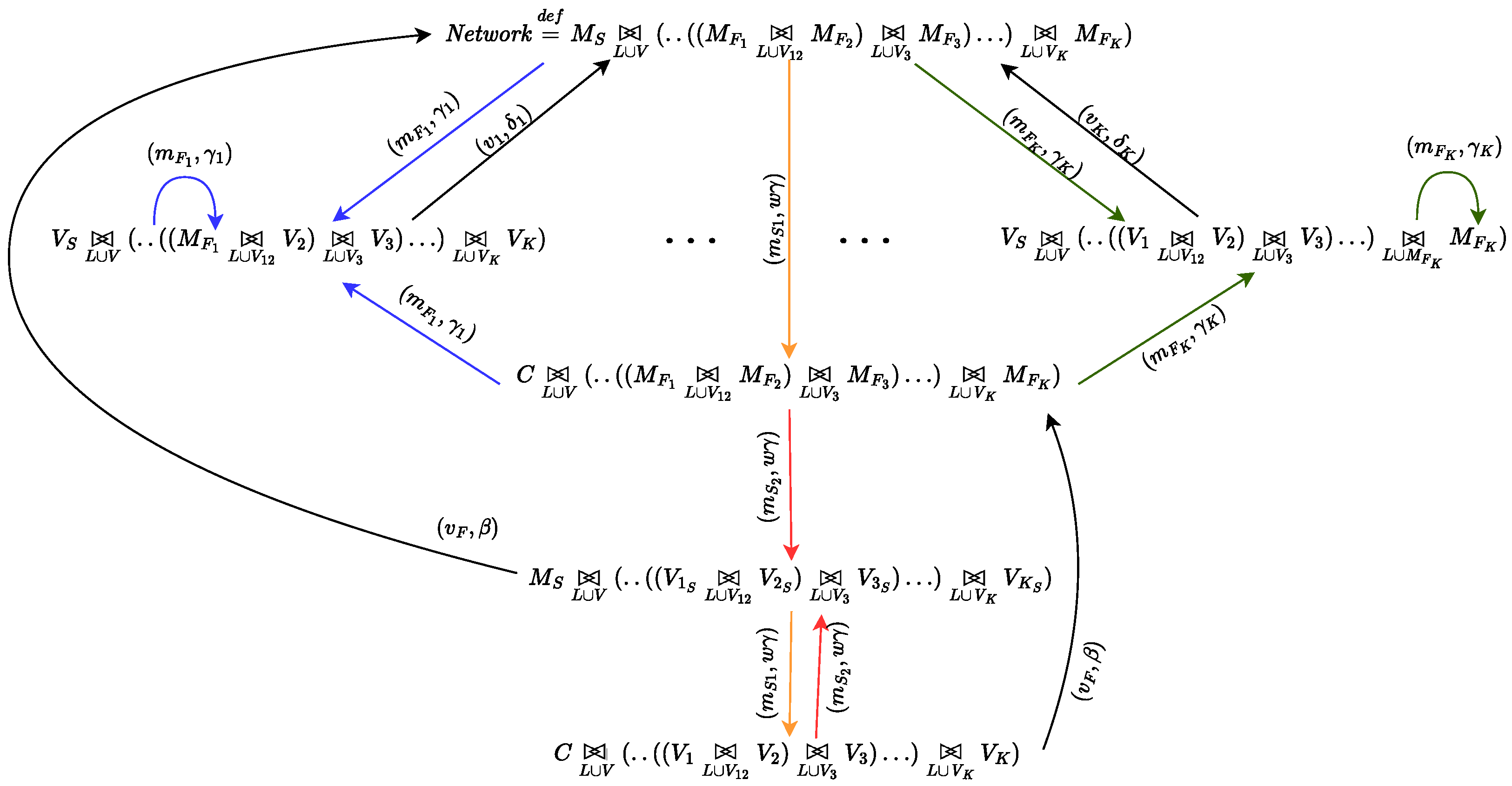
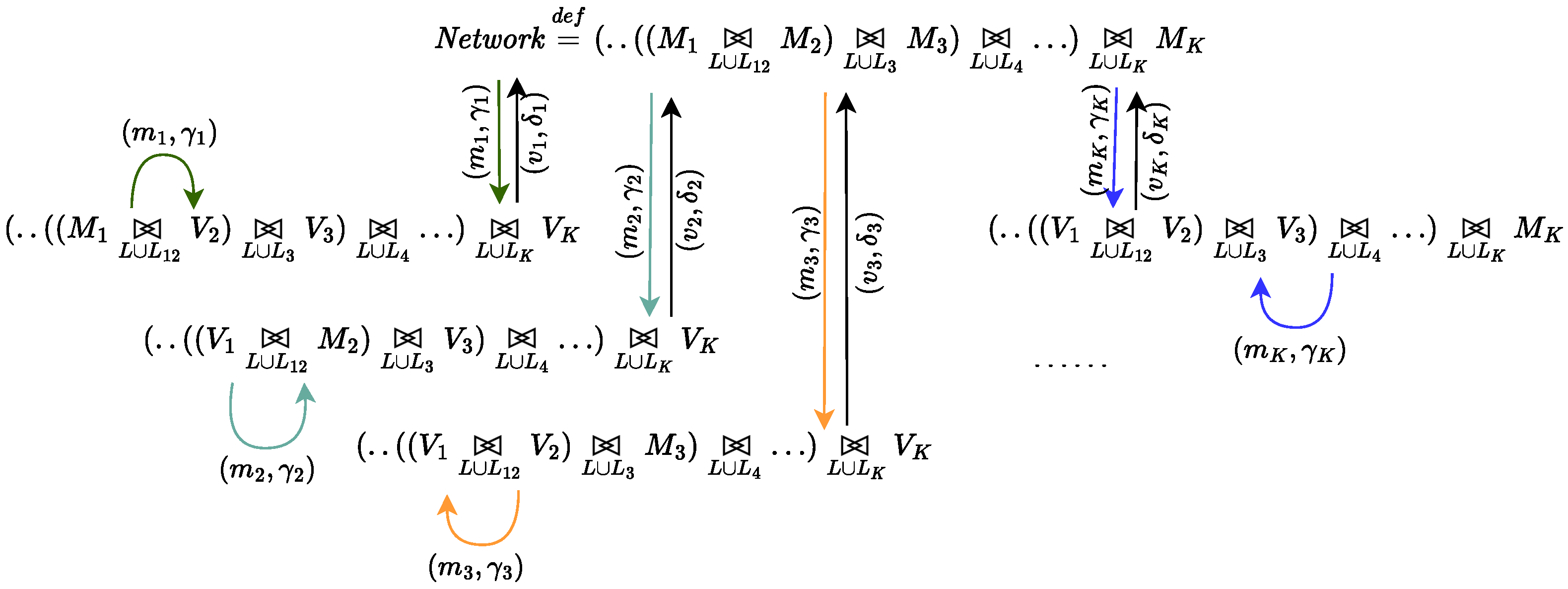
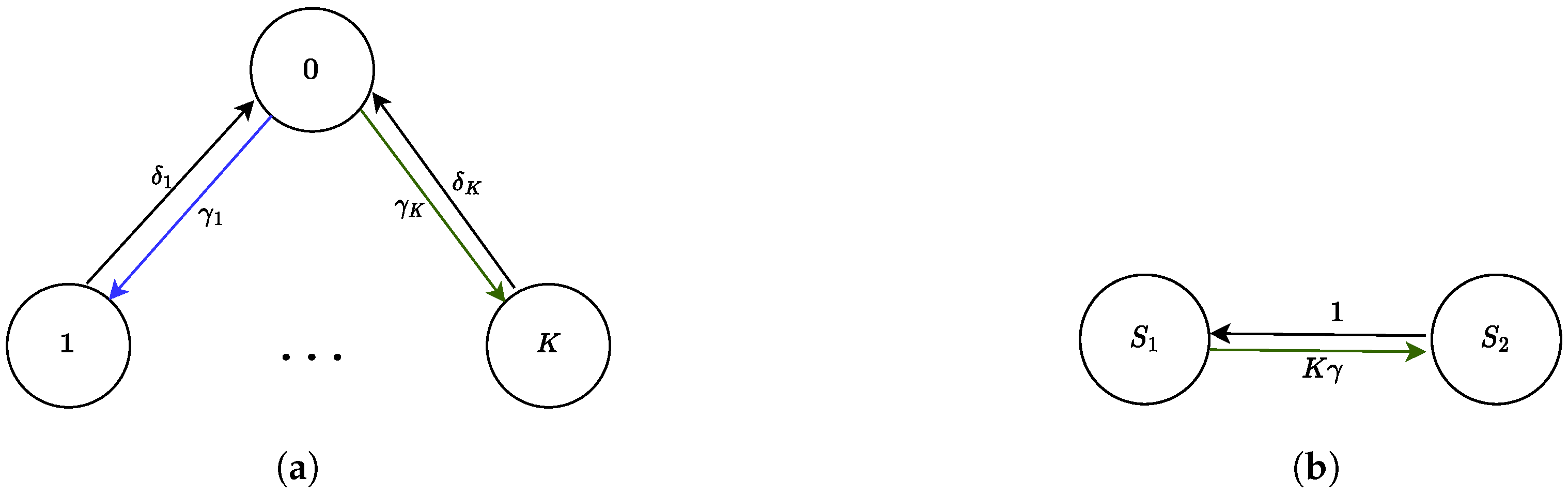
4.1. The Process Algebra PEPA

In this section, we aim to provide a concise overview of Performance Evaluation Process Algebra (PEPA) and shed light on its notable advantages. One of the primary strengths of PEPA lies in its compositional nature. This inherent compositional quality allows for a modular and scalable approach in modeling complex systems. Further, each PEPA specification corresponds to an underlying stochastic process that, under specific assumptions, takes the form of a continuous-time Markov process.

The practical utility of PEPA is enhanced by the availability of a dedicated tool seamlessly integrated into the Eclipse environment, known as the PEPA Eclipse Plug-in [43]. This tool facilitates the application of PEPA, offering a user-friendly environment for modeling and analysis within the Eclipse framework.

A fundamental aspect of a PEPA system specification is its representation as a collection of active agents or components. These components collaboratively engage in activities to collectively shape the overall system behavior. This cooperative behavior is encapsulated by the interaction of components and their respective activities, forming a structured framework for system analysis.

Importantly, the behavior of each individual component within the PEPA framework is characterized by its activities, providing a nuanced understanding of its role within the larger system context. Moreover, the influence of the environment on each component adds a layer of realism to the model, accounting for external factors that may impact the system dynamics.

To facilitate a clear and standardized representation, the syntax for PEPA terms is rigorously defined by a specific grammar as described below:

$$\begin{array}{cc}\hfill & P::=P\stackrel{⊳⊲}{L}P|P/L|SS::=(\alpha ,r).S|S+S|A\hfill \end{array}$$

In this context, the symbols used carry specific meanings within the framework of PEPA. The variable S denotes a sequential component, highlighting a distinct, ordered execution of activities. On the other hand, the variable P represents a model component, which can be obtained as the cooperation of sequential terms, signifying cooperative behavior among them. The operators in PEPA hold distinctive meanings. For instance, $(\alpha ,r).S$ denotes an operation where the activity $(\alpha ,r)$ is performed, involving an action type $\alpha$ and a corresponding rate r. Subsequently, the system behaves as P. The operator $P+Q$ signifies a system that can exhibit the behavior of either P or Q. The choice combinator + represents competition between components. The term $P+Q$ enables all the current activities of both P and Q. The first activity to complete distinguishes one of the components, P or Q. The other component of the choice is discarded. The component $P/L$ operates by behaving as P but with a modification: any activity of type within the set L undergoes relabeling with the unknown type $\tau$.

Introducing constants, denoted by symbols like A, involves defining equations, such as $A\stackrel{def}{=}P$. This equation assigns the behavior of the component P to the constant A, providing a means to encapsulate specific system characteristics within constants.

The cooperation combinator $\stackrel{⊳⊲}{L}$ represents an interaction between two components. The interaction is determined by the set of action types L, referred to as the cooperation set. Activities with action types in this set, known as shared activities, require synchronization between the components. It is assumed that components independently proceed with activities whose types do not belong to the cooperation set L. Crucially, the duration of a shared activity is influenced by the rate of the slower participant. If an activity within a component has an unknown rate denoted as ⊤, the rate of the shared activity will align with that of the other component.

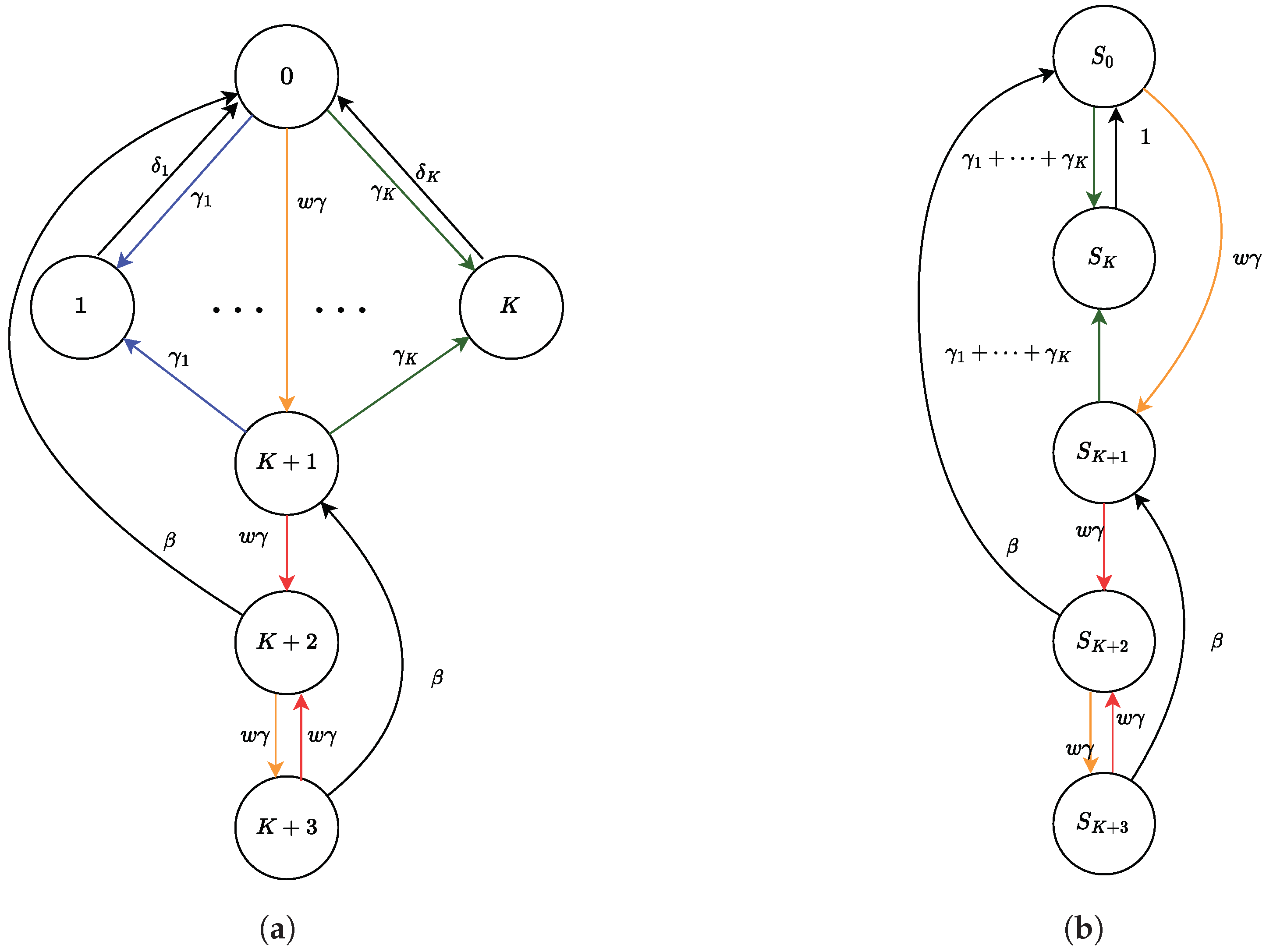
4.2. Selfish Mining in Public Blockchains

The problem of selfish mining in public blockchains (see, e.g., [44,45,46,47,48]) arises when a minority mining pool adopts a strategic approach to maximize its rewards at the expense of other miners. This attack strategy involves the mining pool keeping its successfully mined blocks private, creating a fork in the blockchain. Meanwhile, honest miners continue to mine on the public chain, unaware of the pool’s private branch. As the selfish miners discover more blocks, they strengthen their lead on the public chain and continue to keep their blocks secret. When the public branch approaches the pool’s private branch in length, the selfish miners reveal blocks from their private chain to the public one, causing the public chain to become the shorter branch and their private chain to become the longer one. This results in a waste of resources for honest miners and can lead to a higher number of forks in the blockchain, impacting its performance and security. The selfish mining attack is a significant concern in blockchain systems and requires careful analysis and consideration to develop more robust and efficient solutions.

In the rest of this paragraph, we introduce a PEPA model tailored for the analysis of the selfish mining attack. The model we are about to delineate represents a generalization of the one outlined in [26]. In contrast to the assumptions made in [26], where all miners possess identical computational capabilities for both mining and verification phases, we extend our model to accommodate variations in miners’ computational powers. Consequently, the rates at which miners mine or verify blocks may differ. This adjustment mirrors a more realistic configuration of the blockchain state, enabling us to delve into real-world scenarios with greater precision and relevance. It is important to note that the case study presented in this paper is different from the one discussed in [26]. Our focus encompasses an examination of how the verification time influences the effectiveness of the selfish mining strategy. This consideration becomes particularly significant in the context of the evolving landscape of blockchain technology, notably with the advent of smart contracts. As outlined in seminal work [45], the impact of verification time on selfish mining strategies may not be negligible, rendering our model applicable to a broader spectrum of scenarios.

Our investigation specifically centers on the relationship between verification times and the advantages gained by selfish miners. To elaborate further, we present a PEPA model designed for a blockchain network utilizing a Proof-of-Work (PoW) consensus mechanism. This model accounts for a coalition of fair miners alongside a single selfish miner. Each miner, denoted as $M_i$, operates with an individual computational power represented by ${\gamma }_i$ and verifies blocks with a time frame following an exponentially distributed pattern, with a mean duration of ${\beta }_i^{-1}$.

In

Table 1. PEPA model of a network with K fair miners.

$M_i$	$\stackrel{def}{=}$	$(m_i,{\gamma }_i).M_i+{\displaystyle \sum _{j\ne i}}(m_j,\top ).V_i$
$V_i$	$\stackrel{def}{=}$	${\displaystyle \sum _{j\ne i}}(v_j,{\beta }_i).M_i+{\displaystyle \sum _{j\ne i}}(m_j,\top ).V_i$
$\mathit{Network}$	$\stackrel{def}{=}$	$(..\left(\left(M_1\stackrel{⊳⊲}{L\cup L_{12}}{M}_2\right)\stackrel{⊳⊲}{L\cup L_3}\right)\stackrel{⊳⊲}{L\cup L_4}\cdots )\stackrel{⊳⊲}{L\cup {\mathit{L}}_{\mathit{K}}}{M}_K$
where		$i,j\in \{1,\cdots ,K\}$ and $L=\{m_1,\cdots ,m_K\},L_{12}=\{v_3,\cdots ,v_K\},$
		$L_j=\{v_1,\dots ,v_K\}\setminus \left\{v_j\right\}\mathrm{for} j\ge 3$

, we report the specification of a network composed of $K\ge 3$ fair miners.

Let us inspect the behavior of a single fair (verifying) miner, say $M_1$.

Miner $M_1$ initiates block mining with action type $m_1$ at a rate of ${\gamma }_1$, subsequently returning to its initial state to commence mining another block. Upon receiving a block from the network via an activity $(m_j,\top )$ where $j\in \{2,\dots ,K\}$, $M_1$ enters the verification process, moving to state $V_1$. Notice that, when $M_1$ announces a block, according to the operational semantics of PEPA, $m_1$ is received by all miners except $M_1$. Thus, all miners moves to state $V_1$, while $M_1$ is still mining. Now, according to the synchronization operation, all miners in $V_1$ synchronize on $\left\{v_1\right\}$, and the block is verified at a rate of ${\delta }_1=min({\beta }_2,{\beta }_3,\cdots ,{\beta }_K)$. Once the verification is completed, all the verifying miners simultaneously move to the mining phase. Importantly, $M_1$ remains capable of receiving new blocks from the network during the verification phase through activities $(m_j,\top )$, where $j\in \{2,\dots ,K\}$.

The derivation graph of the model is depicted in Figure 5, where ${\delta }_1=min({\beta }_2,{\beta }_3,\cdots ,{\beta }_K)$, ${\delta }_2=min({\beta }_1,{\beta }_3,\cdots ,{\beta }_K)$, …, ${\delta }_K=min({\beta }_1,{\beta }_2,\cdots ,{\beta }_{K-1})$.

The continuous-time Markov chain underlying the system is depicted in Figure 6a, with states $\{0,1,\dots ,K\}$ where 0 denotes the state of the network in which all miners are mining and $j\in \{1,\dots ,K\}$ denotes the state in which $M_j$ is mining while all the other miners are verifying. It would be interesting to aggregate fair miners into a fair environment according to a relation $\mathcal{R}$ such that $i\mathcal{R}j$ for all $i,j\in \{1,\dots ,K\}$. By applying Theorem 4, one can easliy find that the maximum proportional lumpability for this system with respect to $\mathcal{R}$ is the one induced by the partition:

• $\begin{array}{ccc}{S}_1\hfill & =& \left\{0\right\}\hfill \\ S_2\hfill & =& \{1,\cdots ,K\}\hfill \end{array}$

and the function $\kappa$ such that for each state $s\in S_2$, $\kappa \left(s\right)=q\left(s\right)$, while for $s\in S_1$, $\kappa \left(s\right)=1$. The resulting aggregated CTMC is represented in Figure 6b. As the number of miners in a blockchain can be significantly high, an aggregated model can prove useful in reducing the state space and efficiently calculating performance indices of interest.

Let us now consider a scenario where a network includes a selfish mining pool exercising control with hash power $w\gamma$, utilizing action types $m_{S_1}$ and $m_{S_2}$ for block mining. The PEPA specification for this network, comprising K honest miners and one selfish miner ($M_S$ representing the mining pool), is detailed in

Table 2. PEPA model of a network with K fair miners and one selfish pool $M_S$.

$M_{F_i}$	$\stackrel{def}{=}$	$(m_{F_i},{\gamma }_i).M_{F_i}+{\displaystyle \sum _{j\ne i}}(m_{F_j},\top ).V_i+(m_{S_2},\top ).V_{i_S}$
$V_i$	$\stackrel{def}{=}$	${\displaystyle \sum _{j\ne i}}(v_j,{\beta }_j).M_{F_i}+{\displaystyle \sum _{j\ne i}}(m_{F_j},\top ).V_i$
$V_{i_S}$	$\stackrel{def}{=}$	$(v_S,\beta ).M_{F_i}+(m_{S_2},\top ).V_{i_S}$
$M_S$	$\stackrel{\mathit{def}}{=}$	$(m_{S_1},w\gamma ).C+{\displaystyle \sum _i}(m_{F_i},\top ).V_S$
C	$\stackrel{\mathit{def}}{=}$	$(m_{S_2},w\gamma ).M_S+{\displaystyle \sum _i}(m_{F_i},\top ).V_S$
$V_S$	$\stackrel{\mathit{def}}{=}$	${\displaystyle \sum _i}(v_i,\beta ).M_S+{\displaystyle \sum _{j\ne i}}(m_{F_j},\top ).V_S$
$\mathit{Network}$	$\stackrel{def}{=}$	$M_S\stackrel{⊳⊲}{L\cup V}(..\left(\left(M_{F_1}\stackrel{⊳⊲}{L\cup V_{12}}{M}_{F_2}\right)\stackrel{⊳⊲}{L\cup V_3}{M}_{F_3}\right)\cdots )\stackrel{⊳⊲}{L\cup {\mathit{V}}_{\mathit{K}}}{M}_{F_K})$
where		$i,j\in \{1,\cdots ,K\}$ and $L=\{m_{S_2},m_1,\cdots ,m_K\},V=\{v_1,\cdots ,v_K\},$
		$V_{12}=\{v_S,v_3,\cdots ,v_K\},V_j=\{v_S,v_1,\dots ,v_K\}\setminus \left\{v_j\right\}\mathrm{for} j\ge 3$

. The action type $m_{S_1}$ denotes the first block privately mined by the selfish pool, creating a separate branch, while $m_{S_2}$ represents the second successful block. Upon the production of the second block, two blocks are revealed from the private branch to the public, prompting the rest of the network to transition from the shorter public branch to the newly disclosed blocks. This behavior is reflected in the model, where all network nodes align on the action type $v_S$ upon the announcement of the selfish pool’s second block.

Note that, for modeling simplicity, the selfish miner discloses two blocks from the private branch to the public. However, it is important to acknowledge that the model can be expanded to accommodate a more extended queue of blocks.

Figure 7 represents the derivation graph of the model presented in Table 2, while the Markov process corresponding to the system with K fair components and one selfish pool is represented in Figure 8a. Also in this case, if we define a relation $\mathcal{R}$ among states such that $i\mathcal{R}j$ for all $i,j\in 1,\dots ,K$, this would enable the aggregation of all fair miners into a fair environment. Indeed, by applying Theorem 4, one can find that the maximum proportional lumpability contained in $\mathcal{R}$ is the one induced by the state partition:

• $\begin{array}{ccc}{S}_0\hfill & =& \left\{0\right\}\hfill \\ S_K\hfill & =& \{1,\cdots ,K\}\hfill \\ S_{K+1}\hfill & =& \{K+1\}\hfill \\ S_{K+2}\hfill & =& \{K+2\}\hfill \\ S_{K+3}\hfill & =& \{K+3\}\hfill \end{array}$

and the function $\kappa$ such that for each state $s\in S_K$, $\kappa \left(s\right)=q\left(s\right)$, while for $s\in S_0\cup S_{K+1}\cup S_{K+2}\cup S_{K+3}$, $\kappa \left(s\right)=1$. Thus, we can analyze the aggregated Markov chain represented in Figure 8b and, by Theorems 1 and 2, we can compute the exact solution to the original model.

The symbolic expression of the steady-state probabilities of the Markov chain underlying the lumped network depicted in Figure 8b are:

$$\pi \left(S_0\right)={\displaystyle \frac{{\beta }^2(\mathsf{\Gamma }+w\gamma )+\beta w\gamma (2\mathsf{\Gamma }+\gamma ))}{G}},\pi \left(S_k\right)={\displaystyle \frac{{\beta }^2\mathsf{\Gamma }(\mathsf{\Gamma }+2w\gamma )+\beta \mathsf{\Gamma }w\gamma (2\mathsf{\Gamma }+3\gamma ))}{G}}$$

$$\pi \left(S_{K+1}\right)={\displaystyle \frac{w\gamma \beta (\beta +2w\gamma )}{G}},\pi \left(S_{K+2}\right)={\displaystyle \frac{w{\gamma }^2(\beta +w\gamma )}{G}},\pi \left(S_{K+3}\right)={\displaystyle \frac{w{\gamma }^3}{G}},$$

where $\mathsf{\Gamma }={\gamma }_1+\dots ,{\gamma }_K$, while G is the normalizing constant

$$G={\beta }^2\mathsf{\Gamma }(1+\mathsf{\Gamma })+2\beta (1+\mathsf{\Gamma })(\beta +\mathsf{\Gamma })w\gamma +\beta (4+3\mathsf{\Gamma })w{\gamma }^2+2w{\gamma }^3.$$

By applying Theorem 1, we derive the steady-state probability of the original system; in particular, referring to Figure 8, we obtain:

$$\pi \left(0\right)=\pi \left(S_0\right)=,\pi (K+1)=\pi \left(S_{K+1}\right),\pi (K+2)=\pi \left(S_{K+1}\right),\pi (K+3)=\pi \left(S_{K+3}\right)$$

$$\pi \left(i\right)=\frac{\beta {\prod }_{j=1,j\ne i}^K{\delta }_j{\gamma }_i(\beta \mathsf{\Gamma }+2(\beta +\mathsf{\Gamma })w\gamma +3w{\gamma }^2)}{G}.$$

5. Conclusions

In this study, we have delved into the concept of proportional lumpability and have introduced three distinct characterizations of this novel notion. These characterizations have laid the groundwork for the development of an efficient algorithm designed to automatically check the property of proportional lumpability for, even complex, CTMCs.

The first characterization, as outlined in [21], provides a streamlined method for verifying whether a given relation aligns with proportional lumpability. Building upon this, a second characterization presented in [25] enables the creation of an algorithm for computing proportional lumpability by iteratively refining an initial relation. In this paper. we introduced a novel characterization that significantly enhances computational efficiency, leading to the development of an algorithm for proportional lumpability with a time complexity of $O\left(\right|\mathcal{S}{|}^{2}log\left|\mathcal{S}\right|)$.

To demonstrate the efficacy of proportional lumpability, we conducted an extensive case study akin to the approach outlined in [26]. Specifically, we expanded upon the findings in [26] by analyzing a strongly lumpable model meticulously designed to probe selfish mining behaviors within the context of a public blockchain. The model examined in this paper represents an extended, more general version of the one presented in [26], tailored to capture a more realistic depiction of the blockchain state under investigation. Unlike the assumptions in [26], where all miners are assumed to possess identical computational capabilities for both mining and verification phases, our extended model acknowledges variations in miners’ computational powers. This adjustment offers a more authentic portrayal of the blockchain state, enabling a deeper exploration of real-world scenarios with enhanced accuracy and relevance.

It is crucial to emphasize that the case study presented in this paper diverges from the one discussed in [26]. Our primary focus revolves around investigating how verification time influences the efficacy of the selfish mining strategy. This examination assumes particular importance in the context of the dynamic landscape of blockchain technology, especially with the emergence of smart contracts. As highlighted in seminal work such as [45], the impact of verification time on selfish mining strategies cannot be underestimated, thereby rendering our model applicable to a wider array of scenarios.

Our objective is to offer valuable insights into the concept of proportional lumpability and highlight the broader applications of partition refinement techniques.

As part of our future research endeavors, we aim to explore the possibility of further relaxing the definition of proportional lumpability by introducing approximated semantics, aligning with the spirit of the proposed approaches, e.g., in [49,50,51,52,53]. This future direction aims to enhance the flexibility and applicability of proportional lumpability in various modeling scenarios.

Furthermore, we aim to delve into the concept of component substitution as outlined in [54], specifically for approximating solutions of stochastic models expressed within the framework of Performance Evaluation Process Algebra (PEPA). This approach is introduced to tackle the computational complexity inherent in analyzing PEPA models. The proposed method involves substituting certain components within the models to simplify the analysis process, potentially leading to more efficient and scalable solutions. This methodology hinges upon the notion of behavioral independence [55] to delineate specific restricted classes of models. Essentially, this property affirms that the actions of a specific group of components within a model are unaffected by the actions of other components. This characteristic serves as a valuable means of discerning independent and semi-independent behaviors. The authors suggest substituting a component in a model with a simplified version of itself. This streamlined component maintains the same interactions as the original but usually has fewer states. As a result, the ensuing model generates a significantly smaller Continuous-Time Markov Chain (CTMC), simplifying the solution process. However, determining the transition rates within the simplified component is often challenging. Therefore, an iterative approach, in the spirit of the one proposed in [56], is employed to converge between two or more reduced models. As a future work, we plan to investigate a variant of component substitution grounded in the concept of proportional lumpability. This endeavor will enable us to leverage the findings presented in this paper to efficiently compute an exact solution for the model under consideration. This strategy is in line with the overarching goal of improving the practical usability of PEPA models within real-world systems, thus aiding in the optimization of performance evaluation procedures in computer and digital systems.

References

1. Molloy, M.K. Performance Analysis Using Stochastic Petri Nets. IEEE Trans. Comput. 1982, 31, 913–917. [Google Scholar] [CrossRef]
2. Valk, R.; Vidal-Naquet, G. Petri nets and regular languages. J. Comput. Syst. Sci. 1981, 23, 299–325. [Google Scholar] [CrossRef]
3. Plateau, B. On the stochastic structure of parallelism and synchronization models for distributed algorithms. Sigmetrics Perf. Eval. Rev. 1985, 13, 147–154. [Google Scholar] [CrossRef]
4. Fourneau, J.M.; Plateau, B.; Stewart, W.J. Product form for stochastic automata networks. In Proceedings of the ValueTools 2007 Conference, ICST, Brussels, Belgium, 22–27 October 2007; pp. 1–10. [Google Scholar]
5. Balsamo, S.; Marin, A. Queueing Networks in Formal methods for performance evaluation. In LNCS; Springer: Berlin/Heidelberg, Germany, 2007; Chapter 2; pp. 34–82. [Google Scholar] [CrossRef]
6. Lazowska, E.D.; Zahorjan, J.L.; Graham, G.S.; Sevcick, K.C. Quantitative System Performance: Computer System Analysis Using Queueing Network Models; Prentice Hall: Englewood Cliffs, NJ, USA, 1984. [Google Scholar]
7. Hermanns, H. Interactive Markov Chains; Springer: Berlin/Heidelberg, Germany, 2002. [Google Scholar] [CrossRef]
8. Hillston, J. A Compositional Approach to Performance Modelling; Cambridge University Press: Cambridge, UK, 1996. [Google Scholar] [CrossRef]
9. Schweitzer, P. Aggregation Methods for Large Markov Chains. In Proceedings of the International Workshop on Computer Performance and Reliability, Pisa, Italy, 26–30 September 1983; pp. 275–286. [Google Scholar]
10. Stewart, G. Computable error bounds for aggregated Markov chains. J. ACM 1983, 30, 271–285. [Google Scholar] [CrossRef]
11. Kemeny, J.G.; Snell, J.L. Finite Markov Chains; Springer: Berlin/Heidelberg, Germany, 1976. [Google Scholar] [CrossRef]
12. Baarir, S.; Dutheillet, C.; Haddad, S.; Iliè, J.M. On the use of exact lumping in partially symmetrical Well-formed Petri Nets. In Proceedings of the International Conference on the Quantitative Evaluaiton of Systems (QEST’05), Torino, Italy, 19–22 September 2005; pp. 23–32. [Google Scholar] [CrossRef]
13. Buchholz, P. Exact and Ordinary lumpability in finite Markov chains. J. Appl. Probab. 1994, 31, 59–75. [Google Scholar] [CrossRef]
14. Kant, K. Introduction to Computer System Performance Evaluation; McGraw-Hill: New York, NY, USA, 1992. [Google Scholar]
15. Franceschinis, G.; Muntz, R. Bounds for quasi-lumpable Markov chains. Perform. Eval. 1994, 20, 223–243. [Google Scholar] [CrossRef]
16. Courtois, P.J.; Semal, P. Computable Bounds for Conditional Steady-State Probabilities in Large Markov Chains and Queueing Models. IEEE J. Sel. Areas Commun. 1986, 4, 926–937. [Google Scholar] [CrossRef]
17. Franceschinis, G.; Muntz, R. Computing Bounds for the Performance Indices of Quasi-Lumpable Stochastic Well-Formed Nets. IEEE Trans. Softw. Eng. 1994, 20, 516–525. [Google Scholar] [CrossRef]
18. Baarir, S.; Beccuti, M.; Dutheillet, C.; Franceschinis, G. From partially to fully lumped Markov chains in stochastic well formed Petri nets. In Proceedings of the Valuetools 2009 Conference, Pisa, Italy, 20–22 October 2009; ACM: New York, NY, USA, 2009; p. 44. [Google Scholar] [CrossRef]
19. Milios, D.; Gilmore, S. Component aggregation for PEPA models: An approach based on approximate strong equivalence. Perform. Eval. 2015, 94, 43–71. [Google Scholar] [CrossRef]
20. Marin, A.; Piazza, C.; Rossi, S. Proportional Lumpability. In Proceedings of the International Conference on Formal Modeling and Analysis of Timed Systems, FORMATS, Amsterdam, The Netherlands, 27–29 August 2019; Springer: Berlin/Heidelberg, Germany, 2019; pp. 265–281. [Google Scholar] [CrossRef]
21. Marin, A.; Piazza, C.; Rossi, S. Proportional Lumpability and Proportional Bisimilarity. Acta Inform. 2021, 59, 211–244. [Google Scholar] [CrossRef]
22. Ledoux, J. A necessary condition for weak lumpability in finite Markov processes. Oper. Res. Lett. 1993, 13, 165–168. [Google Scholar] [CrossRef]
23. Kuo, J.; Wei, J. Lumping analysis in monomolecular reaction systems. analysis of approximately lumpable system. Ind. Eng. Chem. Fundam. 1969, 8, 124–133. [Google Scholar] [CrossRef]
24. Li, G.; Rabitz, H. A general analysis of exact lumping in chemical kinetics. Chem. Eng. Sci. 1989, 44, 1413–1430. [Google Scholar] [CrossRef]
25. Piazza, C.; Rossi, S. Reasoning about Proportional Lumpability. In Proceedings of the Quantitative Evaluation of Systems, Paris, France, 23–27 August 2021; Springer: Berlin/Heidelberg, Germany, 2021; Volume 12846, pp. 372–390. [Google Scholar] [CrossRef]
26. Smuseva, D.; Marin, A.; Rossi, S. Selfish Mining in Public Blockchains: A Quantitative Analysis. In Proceedings of the EAI International Conference on Performance Evaluation Methodologies and Tools, Crete, Greece, 6–7 September 2023; Springer: Berlin/Heidelberg, Germany, 2023; pp. 18–32. [Google Scholar] [CrossRef]
27. Ross, S.M. Stochastic Processes, 2nd ed.; John Wiley & Sons: Hoboken, NJ, USA, 1996. [Google Scholar]
28. Taylor, H.M.; Karlin, S. An Introduction to Stochastic Modeling; Academic Press: Cambridge, MA, USA, 1998; Chapter IX. [Google Scholar]
29. Jacobi, M.N. A robust spectral method for finding lumpings and meta stable states of non-reversible Markov chains. Elect. Trans. Numer. Anal. 2010, 37, 296–306. [Google Scholar]
30. Derisavi, S.; Hermanns, H.; Sanders, W.H. Optimal state-space lumping in Markov chains. Elsevier Inf. Process. Lett. 2003, 87, 309–315. [Google Scholar] [CrossRef]
31. Baarir, S.; Beccuti, M.; Dutheillet, C.; Franceschinis, G.; Haddad, S. Lumping partially symmetrical stochastic models. Perform. Eval. 2011, 68, 21–44. [Google Scholar] [CrossRef]
32. Sumita, U.; Rieders, M. Lumpability and time-reversibility in the aggregation-disaggregation method for large Markov chains. Commun. Stat. Stoch. Models 1989, 5, 63–81. [Google Scholar] [CrossRef]
33. Wei, J.; Kuo, J.C. Lumping analysis in monomolecular reaction systems. Analysis of the exactly lumpable system. Ind. Eng. Chem. Fundam. 1969, 8, 114–123. [Google Scholar] [CrossRef]
34. Tomlin, A.S.; Li, G.; Rabitz, H.; Tóth, J. The effect of lumping and expanding on kinetic differential equations. SIAM J. Appl. Math. 1997, 57, 1531–1556. [Google Scholar] [CrossRef]
35. Frostig, E. Jointly optimal allocation of a repairman and optimal control of service rate for machine repairman problem. Eur. J. Oper. Res. 1999, 116, 274–280. [Google Scholar] [CrossRef]
36. Hooghiemstra, G.; Koole, G. On the convergence of the power series algorithm. Perform. Eval. 2000, 42, 21–39. [Google Scholar] [CrossRef]
37. Katehakis, M.; Derman, C. Optimal Repair Allocation in a Series System. Math. Oper. Res. 1984, 9, 615–623. [Google Scholar] [CrossRef]
38. Katehakis, M.; Smit, L. A successive lumping procedure for a class of markov chains. Probab. Eng. Informational Sci. 2012, 26, 483–508. [Google Scholar] [CrossRef]
39. Ungureanu, V.; Melamed, B.; Katehakis, M.; Bradford, P. Deferred Assignment Scheduling in Cluster-Based Servers. Clust. Comput. 2006, 9, 57–65. [Google Scholar] [CrossRef]
40. Valmari, A.; Franceschinis, G. Simple O(m logn) Time Markov Chain Lumping. In Proceedings of the International Conference on TACAS, Edinburgh UK, 15–19 July 2010; Springer Verlag: Berlin/Heidelberg, Germany, 2010; Volume 6015, pp. 38–52. [Google Scholar] [CrossRef]
41. Groote, J.F.; Rivera Verduzco, J.; De Vink, E.P. An Efficient Algorithm to Determine Probabilistic Bisimulation. Algorithms 2018, 11, 131. [Google Scholar] [CrossRef]
42. Hillston, J.; Marin, A.; Piazza, C.; Rossi, S. Persistent stochastic non-interference. Fundam. Informaticae 2021, 181, 1–35. [Google Scholar] [CrossRef]
43. Tribastone, M.; Duguid, A.; Gilmore, S. The PEPA Eclipse Plug-in. Perf. Eval. Rev. 2009, 36, 28–33. [Google Scholar] [CrossRef]
44. Carlsten, M.; Kalodner, H.; Weinberg, S.M.; Narayanan, A. On the instability of bitcoin without the block reward. In Proceedings of the ACM SIGSAC Conference on Computer and Communications Security, Vienna, Austria, 24–28 October 2016; pp. 154–167. [Google Scholar] [CrossRef]
45. Eyal, I.; Sirer, E.G. Majority is not enough: Bitcoin mining is vulnerable. Commun. ACM 2018, 61, 95–102. [Google Scholar] [CrossRef]
46. Göbel, J.; Keeler, H.P.; Krzesinski, A.E.; Taylor, P.G. Bitcoin blockchain dynamics: The selfish-mine strategy in the presence of propagation delay. Perform. Eval. 2016, 104, 23–41. [Google Scholar] [CrossRef]
47. Wright, C.S. The Fallacy of the Selfish Miner in Bitcoin: An Economic Critique. Soc. Sci. Res. Netw. 2018. [Google Scholar] [CrossRef]
48. Motlagh, S.G.; Mišić, J.; Mišić, V.B. The Impact of Selfish Mining on Bitcoin Network Performance. IEEE Trans. Netw. Sci. Eng. 2021, 8, 724–735. [Google Scholar] [CrossRef]
49. Pattipati, K.R.; Kostreva, M.M.; Teele, J.L. Approximate mean value analysis algorithms for queuing networks: Existence, uniqueness, and convergence results. J. ACM 1990, 37, 643–673. [Google Scholar] [CrossRef]
50. Chandy, K.M.; Hergox, U.; Woo, L. Approximate Analysis of General Queueing Networks. IBM J. Res. Dev. 1975, 19, 43–49. [Google Scholar] [CrossRef]
51. Miner, A.S.; Ciardo, G.; Donatelli, S. Using the exact state space of a Markov model to compute approximate stationary measures. In Proceedings of the 2000 ACM SIGMETRICS International Conference on Measurement and Modeling of Computer Systems, New York, NY, USA, 18–21 June 2000; pp. 207–216. [Google Scholar] [CrossRef]
52. Gilmore, S.; Hillston, J.; Ribaudo, M. An Efficient Algorithm for Aggregating PEPA Models. IEEE Trans. Softw. Eng. 2001, 27, 449–464. [Google Scholar] [CrossRef]
53. Casagrande, A.; Dreossi, T.; Piazza, C. Hybrid Automata and ϵ-Analysis on a Neural Oscillator. In Proceedings of the Proceedings First International Workshop on Hybrid Systems and Biology, HSB, Newcastle Upon Tyne, UK, 3 September 2012; Volume 92, pp. 58–72. [Google Scholar] [CrossRef]
54. Thomas, N.; Bradley, J.T.; Thornley, D.J. Approximate solution of PEPA models using component substitution. In Proceedings of the IEE Proceedings—Computers and Digital Technique; IET Digital Library: Stevenage, UK, 2023; Volume 150, pp. 67–74. [Google Scholar] [CrossRef]
55. Thomas, N. Behavioural independence and control in PEPA. In Proceedings of the First Workshop on Process Algebra with Stochastic Timed Activities (PASTA’02), Edinburgh, UK, 2002; Newcastle University Library: Newcastle Upon Tyne, UK, 2002. [Google Scholar]
56. Gribaudo, M.; Sereno, M. Approximation Technique of Finite Capacity Queuing Networks Exploiting Petri Net Analysis. In Proceedings of the Fourth International Workshop on Queuing Networks with Finite Capacity (QNETs 2000), lkley, UK, 20–21 July 2000. [Google Scholar]
Figure 1. CTMC representing the reliability of a system with 3 components.
Algorithms 17 00159 g001
Figure 2. Aggregated CTMC representing the reliability of the system in Figure 1.
Algorithms 17 00159 g002
Figure 3. CTMC for system repair model with common-cause failures.
Algorithms 17 00159 g003
Figure 4. Aggregated CTMC for system repair model with common-cause failures.
Algorithms 17 00159 g004
Figure 5. Derivation graph of the model presented in Table 1.
Algorithms 17 00159 g005
Figure 6. (a) Markov chain underlying the model presented in Table 1 and (b) its aggregation according to proportional lumpability.
Algorithms 17 00159 g006
Figure 7. Derivation graph of the model presented in Table 2.
Algorithms 17 00159 g007
Figure 8. (a) Markov chain underlying the model presented in Table 2 and (b) its aggregation according to proportional lumpability.
Algorithms 17 00159 g008