Evaluating Diffusion Models for the Automation of Ultrasonic Nondestructive Evaluation Data Analysis

Abstract

We develop decision support and automation for the task of ultrasonic non-destructive evaluation data analysis. First, we develop a probabilistic model for the task and then implement the model as a series of neural networks based on Conditional Score-Based Diffusion and Denoising Diffusion Probabilistic Model architectures. We use the neural networks to generate estimates for peak amplitude response time of flight and perform a series of tests probing their behavior, capacity, and characteristics in terms of the probabilistic model. We train the neural networks on a series of datasets constructed from ultrasonic non-destructive evaluation data acquired during an inspection at a nuclear power generation facility. We modulate the partition classifying nominal and anomalous data in the dataset and observe that the probabilistic model predicts trends in neural network model performance, thereby demonstrating a principled basis for explainability. We improve on previous related work as our methods are self-supervised and require no data annotation or pre-processing, and we train on a per-dataset basis, meaning we do not rely on out-of-distribution generalization. The capacity of the probabilistic model to predict trends in neural network performance, as well as the quality of the estimates sampled from the neural networks, support the development of a technical justification for usage of the method in safety-critical contexts such as nuclear applications. The method may provide a basis or template for extension into similar non-destructive evaluation tasks in other industrial contexts.

1. Introduction

Ultrasonic (UT) non-destructive evaluation (NDE) is used in many applications to establish a fitness-for-service argument for components under test [1]. Its usage is widely established in safety-critical contexts such as aviation and nuclear energy [2]. Despite its usefulness, the manual analysis of UT datasets is costly and time-consuming and there is considerable interest in automating the process. This is true for nuclear energy in particular, as ongoing concerns for the environment have sponsored a renewed interest in nuclear energy production as the emissions-free energy it produces may help in stemming the tide of global warming. In order to enhance the cost-effectiveness of nuclear energy relative to emissions-producing alternatives, nuclear plant owner–operators are investigating the use of statistical learning techniques to reduce the financial impact of necessary but costly UT NDE data analysis.

While modern statistical learning methods [3] providing decision support in industrial contexts show great promise, the risk and consequence of failure often prevents their usage in highly regulated safety-critical contexts. It is the failure of such methods to provide guarantees on out-of-distribution performance that most strongly prejudices against their usage in the field where any number of factors may impact or skew the distribution of acquired data away from the training data and perhaps negatively impact performance [4]. Our contribution is to demonstrate a principled usage of a state-of-the-art generative model that trains offline on each dataset independently, and so depends only on the distribution of the data at hand, skirting any dependence on out-of-distribution generalization. We work with generative models based on variational inference that allow us to describe, understand, and proof test performance using probabilistic reasoning that captures the method’s rationale in a way that regulators familiar with probabilistic risk assessment might be comfortable with.

As shown in Figure 1, we summarize a UT data set of ascans as a time series consisting of the peak amplitude response time of flight for each ascan. We express the UT data analysis task, on the time series, in probabilistic terms that relate it to a Conditional Score-Based Diffusion (CSDI) [5] loss function and train a CSDI model to perform the probabilistically specified task. We use the threshold reconstruction error of a Variational Autoencoder trained to encode and decode UT $ascas$ to partition the time series dataset as nominal and anomalous subsets; by ignoring the anomalous subset during training, the dataset distribution is effectively biased towards the nominal distribution. Sampling from the trained model and comparing sampled results to the observed data allows us to identify and quantify deviations from nominal.

The CSDI model is a conditional score-based derivative of DPM first introduced in [6] and reformulated in [7,8]. The CSDI architecture differentiates itself by exhibiting state-of-the-art results for time series data imputation on numerous bench-marks and popular time series performance metrics [5]. We use CSDI to impute or estimate unobserved nominal data in our UT NDE datasets. We investigate opportunities to improve nominal estimates by partitioning training datasets to induce bias towards the nominal distribution.

CSDI is based on DiffWave [9], which in turn is based on a U-Net like architecture [10]. U-Nets consist of a symmetric stacked encoder and decoder network; with the encoder a series of down-sampling blocks, and the decoder a series of up-sampling blocks. Skip connections run between the corresponding blocks of the encoder and decoder. CSDI models are defined as forward and reverse Markov chain processes, where the forward process noises an input data vector, bringing it from the input data distribution at time step $t=0$, to a Gaussian noise vector at time step $t=T$. The reverse process denoises, to bring a sampled noise vector at $t=T$, to the learned approximation of the data distribution at time step $t=0$. During training CSDI optimizes the error on a learned prediction of the noise that must be removed from the data at time step t to bring it to the step-wise denoised data at time step $t-1$. In addition to time step information, CSDI models inject conditional masks, temporal embeddings, and feature embeddings to each up and down sampling block during training. The embeddings and masks get picked up by the attention mechanisms [11] in the residual layers [12] of the U-Net encoder and decoder blocks. The attention mechanisms facilitate the learning of the conditional data distribution.

2. Related Work

Automated Data Analysis of Pressure Tubes, an end-to-end expert system that provides decision support and explainability for automated flaw characterization in UT NDE data taken from PT, is proposed in [13,14,15]. The system is based on deterministic rules and explainability is generated using a tree-based system developed with input from practitioners. Ref. [16] investigates the use of a self-supervised two-stage Decibel Scan (DBSCAN)-based method to identify and cluster anomalies in UT NDE data taken from PT. The first stage clusters on the basis of learned features in the data, the second on the basis of location. A proof-of-concept supervised CNN based architecture is used in [17] to identify flaws in PT UT data. Labels are provided by manual data analysis and training data are down-sampled and concatenated to manage compute requirements. The results suggest that supervised training methods are able to identify suitably labeled flaw regions in UT data, but the results are adversely impacted by noise in the dataset.

All referenced work shares a dependency on labelled data and out of distribution generalization. In the case of [13,14,15] labels and analysis are required in order to generate the set of rules on which the system operates. In the case of [17], labeled data are required to train the neural networks used to identify flaws. The robustness of any system relying on labelled data depends on the amount of labeled data provided; more is considered better. The use of large datasets supports generalization in the type of deep learning systems trained in [17] and will allow rules-based systems, as in [13,14,15], to account for a wider variety of field conditions. The difficulty in terms of real-world applications of sufficient complexity is that field conditions may vary widely and in an unanticipated fashion, so that a dataset of any size cannot be guaranteed to provide the information required for sufficient generalization.

3. UT NDE and Nuclear Fuel Channel Pressure Tubes

A typical Canada Deuterium Uranium (CANDU) reactor contains 480 zirconium alloy Pressure Tubes (PT). Each is approximately 560 mm long, with a diameter of 100 mm and wall thickness around five millimeters. During reactor operation the PT house the reactor fuel. PT operate under high pressure and temperature and experience significant neutron flux. These factors cause the PT to geometrically deform and make thinning and weakening of the pipe wall possible over time. PT are also subject to chemical processes that increase the risk of catastrophic failure due to embrittlement; this is especially relevant in and around evolving cracks, scratches, and fissures in the PT material [18].

The confirmation of PT integrity by way of physical inspection is one risk-mitigation strategy employed by nuclear owner operators to ensure continued safe operation. And so during planned maintenance outages PT are emptied of their fuel and inspected with UT NDE tooling. A primary goal of inspections is to locate and characterize material flaws. Flaws are sudden changes in pipe wall geometry such as those caused by abrasion and wear of reactor fuel bundles and debris interacting with the PT inner diameter surface. Flaws are of interest primarily because regions at the bounding points of their geometry are under increased mechanical stress which enhances the risk of catastrophic failure [18]. In order to monitor and mitigate the risk of such an outcome PT flaws are characterized and a set of criteria are used to determine the risk of each to continued safe reactor operation.

4. Dataset Details

The UT probe acquiring the data is situated on a rotating mechanical head which when centered inside an empty PT, and pushed very slowly down its length as the head spins, allows data acquisition over the entire inner diameter surface of the PT in a tight corkscrew pattern. Our dataset contains 3600 $ascans$ per head rotation, on an axial raster of ∼0.2 mm. In this dataset the subject under test is a calibration fixture, which is a mock PT, scanned before every real PT inspection. The signal response from notches in the fixture is used to verify and tune UT probes to meet inspection quality requirements. Figure 1 provides a detailed look at a portion of our dataset. Each $ascan$ in the dataset is associated with the tool position (axial and rotary) and time of data acquisition. This allows the set to be ordered (and visualized) in time, or position, of acquisition as desired.

For our purposes we reduce the dimensionality of the $ascan$ dataset, summarizing each $ascan$ by the time of flight of its maximum value $t_{pa}$, which we refer to as peak amplitude response time of flight. This is simply the time in $\mathsf{\mu }$s at which the peak value of a given $ascan$ (such as those in the top right column of Figure 1) occurs. Multiplying $t_{pa}$ by the speed of sound v in $D_{2}O$ (deuterium oxide, or heavy water, is the nuclear fuel coolant in a CANDU reactor) gives the round-trip distance between the UT probe and the primary reflector, in this case the calibration fixture inner diameter pipe wall.

We can extract $t_{pa}$ from a given $ascan$ using an $argmax(·)$ function (scientific computing software libraries generally include an $argmax\left(\right)$ function that will return an array’s maximum value and index) operating on the $ascan$ data vector. So, given a set of $ascans$$\mathcal{A}$ with elements a, we construct dataset $\mathcal{X}$ as follows:

$$\mathcal{X}=\left\{argmax\right(a\left)\right|\forall a\in \mathcal{A}\}$$

(1)

where $argmax\left(a\right)$ yields $t_{pa}$ for $a\in \mathcal{A}$.

5. Manual Data Analysis on the Manifold

UT NDE data analysis often involves the identification and characterization of variance from the nominal trend in some set of assumed continuous measured quantities. In fact, the estimation of the difference between an observed and an inferred nominal value constitutes the bulk of UT NDE data analysis effort. In most industrial contexts, anomalies have a relatively low rate of occurrence and this puts discriminative learning methods, which rely on a balance of classes within the dataset, at a disadvantage. As we will demonstrate, generative models like Variational Autoencoders (VAE) and Diffusion Probabilistic Models (DPM) are accommodating in this regard, in that they allow us to leverage the prevalence of the nominal trend within the data to predict a would-be nominal signal where it is unobserved. As an added bonus, the semantics of variational inference lend well to the expression of the UT NDE data analysis task as sampling from learnable distribution, which facilitates a technical justification for the use of generative methods in highly regulated contexts conversant in probabilistic risk assessment.

An extension of the manifold hypothesis [19] is that there exists a set of distinct data-generating factors, each contributing to the distribution of an observed data set [20]. Given this is true, we could say that in some sense the process of manual UT data analysis involves classifying the data caused by these factors as nominal or anomalous and then using the classification to identify and infer a possibly obscured nominal trend. We draw from the concept of data generating factors and assume the existence of two groups of factors in our dataset. A nominal group consisting of all factors supporting the smooth operation of the data-acquisition system over a continuous surface of the material under test. And an anomalous set of data generating factors—those causing spurious or noisy operation in data acquisition and those causing unanticipated discontinuity in the otherwise-continuous properties and features of the material under test.

On the basis of this understanding, we can reframe the task of the analyst as the determination of a partition for nominal and anomalous data and subsequent estimation of the nominal trend on the basis of the nominal information. Ultimately identifying the nominal trend allows the estimation of unobserved nominal data, which in turn supports the estimate of variance from an estimated nominal in observed anomalous data.

Traditional approaches to establish a useful partition may involve some form of data classification and curve fitting. For instance, some threshold may be used to partition observed data, and then some curve fitting technique applied to identify nominal trend. However, accurate identification of the nominal trend is sensitive to the quality of the partition. Given a correct partition the relative ease of identifying nominal trend follows. But, as in Figure 2, heuristic approaches are brittle and fail when the partition mixes support from nominal and anomalous data-generating factors. This detracts from the usefulness of such methods, as the difficulty in diagnosing errors leads to a lack of confidence in results.

6. A Probabilistic Model for UT Data Analysis

Given an ordered set of $ascans$ taken as a UT probe passes over the surface of a test subject. Let dataset $\mathcal{X}$ be the similarly ordered peak amplitude response time of flight of each $ascan$ in the set. Let the ordering provide a one-to-one mapping between each $x\in \mathcal{X}$ and a unique time and position of data acquisition. Define $\mathcal{X}$ as the union of nominal and anomalous data subsets ${\mathcal{X}}^n$ and ${\mathcal{X}}^a$ so that $\mathcal{X}$ is partitioned:

$$\mathcal{X}={\mathcal{X}}^n\cup {\mathcal{X}}^a$$

(2)

Then according to our understanding of data generating factors x is distributed as joint probability

$$x\sim P(x^n,x^a)$$

(3)

where $x^n\in {\mathcal{X}}^n$ and $x^a\in {\mathcal{X}}^a$.

We define dataset ${\mathcal{X}}^u$ with elements $x^u\in {\mathcal{X}}^u$ to allow reference to unobserved nominal data. The $x^u$ are the nominal signals that would have been observed were it not for the occurrence of an anomalous data generating factor. In terms of causality we might conceive of ${\mathcal{X}}^u$ as the observations that would have occurred had we intervened to constrain the effect of anomalous data-generating factors.

We desire estimates for $x^u\in {\mathcal{X}}^u$. An analyst estimates the unobserved nominal data by first classifying observed data as either nominal or anomalous and then estimating unobserved nominal data on the basis of observed local nominal signal. This estimate relies on an inference process that makes strong use of the observed element wise continuity in ${\mathcal{X}}^n$. We model this estimation process as sampling the unobserved nominal with a conditional dependence on the observed nominal:

$$x^u\sim P\left(x^u\right|{\mathcal{X}}^n)$$

(4)

In the unsupervised learning setting we are given no knowledge of membership in ${\mathcal{X}}^n$, ${\mathcal{X}}^a$, or ${\mathcal{X}}^u$. The best we can do directly from the dataset is sample $x^u\sim P\left(x\right|\mathcal{X})$. We believe that with some engineering we can do better than this, and make the reasonable assumption that unobserved nominal data are distributed as the observed nominal so that

$$x^u\sim P\left({\mathcal{X}}^n\right)$$

(5)

Substituting $x^n$ for $x^u$ in Expression (4) gives

$$\begin{array}{c}\hfill x^u\sim P\left(x^n\right|{\mathcal{X}}^n)\end{array}$$

(6)

which, given the assumptions, allows the estimation of ${\mathcal{X}}^u$ by way of some unsupervised generative model trained to sample from $P\left(x^n\right|{\mathcal{X}}^n)$ by training on partitioned dataset $\mathcal{X}$.

Because PT are well maintained, and data are acquired with very strict quality controls, we expect that cardinality $|{\mathcal{X}}^n| \gg |{\mathcal{X}}^a|$. This implies that in general $P\left(x^n\right)\gg P\left(x^a\right)$ and allows us to consider the approximation

$$\begin{array}{c}\hfill x^n\sim P\left(\mathcal{X}\right)\end{array}$$

(7)

This circuitously suggests a model trained on all observed data

$$\begin{array}{c}\hfill x^u\sim P\left(x\right|\mathcal{X})\end{array}$$

(8)

which could also allow the accurate estimation of $x^u\in {\mathcal{X}}^u$. We coin Expression (6) the Nominal Data Model (NDM), and (8) the Observed Data Model (ODM).

7. Diffusion Probabilistic Models

Diffusion Probabilistic Models (DPM) are a class of latent variable models of the form $p_{\theta }\left({\mathbf{x}}_0\right):=\int p_{\theta }\left({\mathbf{x}}_{0:T}\right)d{\mathbf{x}}_{1:T}$ where the data vector ${\mathbf{x}}_0\sim q\left({\mathbf{x}}_0\right)$ is of the same dimension as latent vectors ${\mathbf{x}}_1,...,{\mathbf{x}}_T$ and p is parameterized by $\theta$ [7]. The model chains the input variable vector ${\mathbf{x}}_0$ with the T latent variable vectors and defines a forward and reverse process over the chain. The model architecture presumes a learned Gaussian transition from each vector in the chain to the next, with each transition parameterized by a neural network of input and output dimension equal to the input variable vector. (We assume that the reader is familiar with the semantics and notation that is the lingua franca of variational inference and diffusion processes so that this high-level overview may serve as a refresher. For a full treatment and development of variational inference and VAE, see [21], for Denoising Diffusion Probabilistic Models see [7], and for Conditional Score-Based Diffusion, see [5]).

The approximate posterior $q\left({\mathbf{x}}_{1:T}\right|{\mathbf{x}}_0)$, or forward process, is defined as a Markov chain that transforms input data vectors to a target distribution by gradually adding noise at each of T steps according to a learnable variance schedule ${\beta }_1,...,{\beta }_T$:

$$\begin{array}{ccc}\hfill q\left({\mathbf{x}}_{1:T}\right|{\mathbf{x}}_0)& \hfill :=\prod _{t=1}^{T}q\left({\mathbf{x}}_t\right|{\mathbf{x}}_{t-1}),\hspace{1em}\hspace{1em}\hfill & \hfill q\left({\mathbf{x}}_t\right|{\mathbf{x}}_{t-1}):=\mathcal{N}({\mathbf{x}}_t;\sqrt{1-{\beta }_t}{\mathbf{x}}_{t-1},{\beta }_t\mathbf{I})\end{array}$$

(9)

The reverse process is a joint probability $p_{\theta }\left({\mathbf{x}}_{0:T}\right)$ defined as a Markov chain starting at $p\left({\mathbf{x}}_T\right)=\mathcal{N}({\mathbf{x}}_T;\mathbf{0},\mathbf{I})$ that transforms its input across T learned Gaussian transitions:

$$\begin{array}{ccc}\hfill p_{\theta }\left({\mathbf{x}}_{0:T}\right)& \hfill :=p\left({\mathbf{x}}_T\right)\prod _{t=1}^T{p}_{\theta }\left({\mathbf{x}}_{t-1}\right|{\mathbf{x}}_t),\hspace{1em}\hspace{1em}\hfill & \hfill p_{\theta }\left({\mathbf{x}}_{t-1}\right|{\mathbf{x}}_t):=\mathcal{N}({\mathbf{x}}_{t-1};{\mathit{\mu }}_{\theta }({\mathbf{x}}_t,t),{\Sigma }_{\theta }({\mathbf{x}}_t,t)\mathbf{I})\end{array}$$

(10)

Diffusion models admit closed form expressions for sampling ${\mathbf{x}}_t$ at arbitrary step t. Being differentiable they support training by stochastic gradient descent to optimize the variational lower bound L on negative log likelihood:

$$\begin{array}{c}\hfill \mathbb{E}[-log{p}_{\theta }\left({\mathbf{x}}_0\right)]\le {\mathbb{E}}_q\left[-log\frac{p_{\theta }\left({\mathbf{x}}_{0:T}\right)}{q\left({\mathbf{x}}_{1:T}\right|{\mathbf{x}}_0)}\right]={\mathbb{E}}_q\left[-logp\left({\mathbf{x}}_T\right)-\sum _{t\ge 1}log\frac{p_{\theta }\left({\mathbf{x}}_{t-1}\right|{\mathbf{x}}_t)}{q\left({\mathbf{x}}_t\right|{\mathbf{x}}_{t-1})}\right]:=L\end{array}$$

(11)

where $\mathbb{E}$ is the expectation. Sampling of ${\mathbf{x}}_t$ at arbitrary time step t is achieved as follows:

$$\begin{array}{c}\hfill q\left({\mathbf{x}}_t\right|{\mathbf{x}}_0)=\mathcal{N}({\mathbf{x}}_t;\sqrt{\overline{\alpha }}{\mathbf{x}}_0,(1-{\overline{\alpha }}_t)\mathbf{I})\end{array}$$

(12)

where ${\alpha }_t:=1-{\beta }_t$ and ${\overline{\alpha }}_t:={\prod }_{s=1}^t{\alpha }_s$.

7.1. Denoising Diffusion Probabilistic Models

Denoising Diffusion Probabilistic Models (DDPM) reformulate the variational bound in Equation (11) [7] as follows:

$$\begin{array}{c}\hfill L:={\mathbb{E}}_q\left[D_{KL}(q\left({\mathbf{x}}_T\right|{\mathbf{x}}_0)\left|\right|p\left({\mathbf{x}}_T\right))+\sum _{t>1}{D}_{KL}(q\left({\mathbf{x}}_{t-1}\right|{\mathbf{x}}_t,{\mathbf{x}}_0)\left|\right|p_{\theta }\left({\mathbf{x}}_{t-1}\right|{\mathbf{x}}_t))-log{p}_{\theta }\left({\mathbf{x}}_0\right|{\mathbf{x}}_1)\right]\end{array}$$

(13)

where the forward process variance schedule ${\beta }_t$, which may be learned, is fixed to constants. This removes all learnable parameters from the first term of Equation (13); removing it from consideration during training. The reverse process covariance matrix ${\Sigma }_{\theta }({\mathbf{x}}_t,t)={\sigma }^2\mathbf{I}$ is also set to step dependent unlearned constants; which removes it from consideration during training also. Reparameterizing the sampling procedure in Equation (12) with ${\mathbf{x}}_t({\mathbf{x}}_0,\mathit{ϵ})=\sqrt{{\overline{\alpha }}_t}{\mathbf{x}}_0+\sqrt{1-{\overline{\alpha }}_t}\mathit{ϵ}$ where $\mathit{ϵ}\sim \mathcal{N}(\mathbf{0},\mathbf{I})$ leads to the parameterization

$$\begin{array}{cc}\hfill {\mathit{\mu }}_{\theta }({\mathbf{x}}_t,t)=\frac{1}{{\alpha }_t}\left({\mathbf{x}}_t-\frac{{\beta }_t}{\sqrt{1-{\alpha }_t}}{\mathit{ϵ}}_{\theta }({\mathbf{x}}_t,t)\right),& \hfill {\sigma }_{\theta }({\mathbf{x}}_t,t)={\tilde{\beta }}_t^{1/2},where{\tilde{\beta }}_t=\left\{\begin{array}{c}\hfill \frac{1-{\alpha }_{t-1}}{1-{\alpha }_t}{\beta }_{t}t>1\hfill \\ \hfill {\beta }_{1}t=1\hfill \end{array}\right.\hfill \end{array}$$

(14)

where ${\mathit{ϵ}}_{\theta }$ is a learnable denoising function that reverses the forward process. With this parameterization, the DDPM loss function reduces to

$$\begin{array}{c}\hfill L_{DDPM}\left(\theta \right):={\mathbb{E}}_{t,{\mathbf{x}}_0,\mathit{ϵ}}\left[{\parallel \mathit{ϵ}-{\mathit{ϵ}}_{\theta }(\sqrt{\overline{\alpha }}{\mathbf{x}}_0+\sqrt{1-{\overline{\alpha }}_t}\mathit{ϵ},t)\parallel }^2\right]\end{array}$$

(15)

The DDPM model includes a decoder in the final step of the reverse process to improve sampling. The decoder relies on the linear scaling of data on the range $[-1,1]$ and allows the direct sampling of ${\mathit{\mu }}_{\theta }({\mathbf{x}}_1,1)$ without any addition of noise.

7.2. Conditional Score-Based Diffusion

Conditional Score-Based Diffusion (CSDI) [5] models introduce a conditional into the reverse process of the DDPM as follows:

$$\begin{array}{cc}\hfill p_{\theta }\left({\mathbf{x}}_{0:T}^{ta}\right|{\mathbf{x}}_0^{co})& \hfill :=p\left({\mathbf{x}}_T^{ta}\right)\prod _{t=1}^T{p}_{\theta }\left({\mathbf{x}}_{t-1}^{ta}\right|{\mathbf{x}}_t^{ta},{\mathbf{x}}_0^{co}),{\mathbf{x}}_T^{ta}\sim \mathcal{N}(\mathbf{0},\mathbf{I}),\hfill \end{array}$$

(16)

$$\begin{array}{cc}\hfill p_{\theta }\left({\mathbf{x}}_{t-1}^{ta}\right|{\mathbf{x}}_t^{ta},{\mathbf{x}}_0^{co})& \hfill :=\mathcal{N}({\mathbf{x}}_{t-1}^{ta};{\mathit{\mu }}_{\theta }({\mathbf{x}}_t^{ta},t|{\mathbf{x}}_0^{co}),{\sigma }_{\theta }({\mathbf{x}}_t^{ta},t|{\mathbf{x}}_0^{co})\mathbf{I})\hfill \end{array}$$

(17)

where imputation targets ${\mathbf{x}}_0^{ta}\in {\mathcal{X}}^{ta}$ are unobserved data, and ${\mathbf{x}}_0^{co}\in {\mathcal{X}}^{co}$ are the observed data on which estimates of the unobserved data are made conditional. Introducing a conditional into the expression for ${\mathit{ϵ}}_{\theta }$ in the DDPM parameterization in Equation (14), we arrive at the parameterization for CSDI:

$$\begin{array}{cc}\hfill {\mathit{\mu }}_{\theta }({\mathbf{x}}_t^{ta},t|{\mathbf{x}}_0^{co})=\frac{1}{{\alpha }_t}\left({\mathbf{x}}_t^{ta}-\frac{{\beta }_t}{\sqrt{1-{\alpha }_t}}{\mathit{ϵ}}_{\theta }({\mathbf{x}}_t^{ta},t|{\mathbf{x}}_0^{co})\right)& \end{array}$$

(18)

$$\begin{array}{c}\hfill {\sigma }_{\theta }({\mathbf{x}}_t^{ta},t|{\mathbf{x}}_0^{co})={\tilde{\beta }}_t^{1/2},where{\tilde{\beta }}_t=\left\{\begin{array}{c}\hfill \frac{1-{\alpha }_{t-1}}{1-{\alpha }_t}{\beta }_{t}t>1\hfill \\ \hfill {\beta }_{1}t=1\hfill \end{array}\right.\end{array}$$

(19)

Which implies the corresponding CSDI loss function:

$$\begin{array}{c}\hfill \underset{\theta }{min}L\left(\theta \right):=\underset{\theta }{min}{\mathbb{E}}_{{\mathbf{x}}_0\sim q\left({\mathbf{x}}_0\right),\mathit{ϵ}\sim \mathcal{N}(\mathbf{0},\mathbf{I}),t}{\parallel \mathit{ϵ}-{\mathit{ϵ}}_{\theta }({\mathbf{x}}_t^{ta},t|{\mathbf{x}}_0^{co})\parallel }_2^2\end{array}$$

(20)

CSDI implements a self-supervised learning method, inspired by training in masked language models, which holds back observed data, in an amount determined by the “missing ratio” hyperparameter, as simulated unobserved targets with ground truth. The CSDI architecture uses an attention mechanism with multi-head and fully connected layers to identify temporal and feature dependencies. The feature dependencies are used to generate "side information" that is passed to the gated activation unit in each residual diffusion layer. The diffusion layers are each composed as a U-Net with skip connections all passing information to the final convolutional output layers.

8. Experiments and Results

We seek to interpret results in terms of the probabilistic models developed in Section 6. Where alignment between the models and results gleaned from their implementations will be taken to imply that there exists a principled basis to which we may fix an understanding of performance, and that this may in turn provide the basis for a technical justification of the use of diffusion-based methods in safety-critical contexts. To make relevant observations we begin by constructing a number of datasets to train diffusion models on.

Dataset $\mathcal{X}$ that underlies the NPM and OPM of Expressions (6) and (8), respectively, is defined as a partition ${\mathcal{X}}^n,{\mathcal{X}}^a$ that classifies the data as nominal or anomalous. To test the validity of the probabilistic models, and their DPM based implementations, we generate a collection of datasets each based on a unique partition of the data. We first use manual classification to construct a ground truth dataset ${\mathcal{X}}_{gt}$ with partition formed by ${\mathcal{X}}_{gt}^n$, and ${\mathcal{X}}_{gt}^a$. We then use a method similar to that described in [22] to construct a series of datasets with partitions generated using output from a VAE. Partitions are constructed by first training a VAE to encode and decode the $ascans$ from which dataset $\mathcal{X}$ is derived. Then percentiles of the mean squared error of $ascan$ reconstruction are used as thresholds to partition $\mathcal{X}$ so that the time of flight associated with $ascans$ with a reconstruction error less than the threshold percentile value are classified as nominal, and otherwise anomalous. Thus, given the value of the 90th MSE percentile we construct dataset ${\mathcal{X}}_{0.90}$ the union of ${\mathcal{X}}_{0.90}^n$, and ${\mathcal{X}}_{0.90}^a$. Each of the constructed datasets is then a unique partition over the data.

We test DDPM and CSDI diffusion models on each of the datasets and train them for five epochs. Our implementations of DDPM and CSDI are based on the code provided with [5]. The training of CSDI models requires a missing ratio hyperparameter which is equivalently expressed as the percentage rate of observed data held back as simulated ground truth during training. This percentage regulates the degree to which the conditional mechanism of the model is exercised on the observed nominal data. DDPM models do not exercise a conditional mechanism when training. We test CSDI models on the range of missing data rates $[10\%,20\%,\dots ,50\%]$.

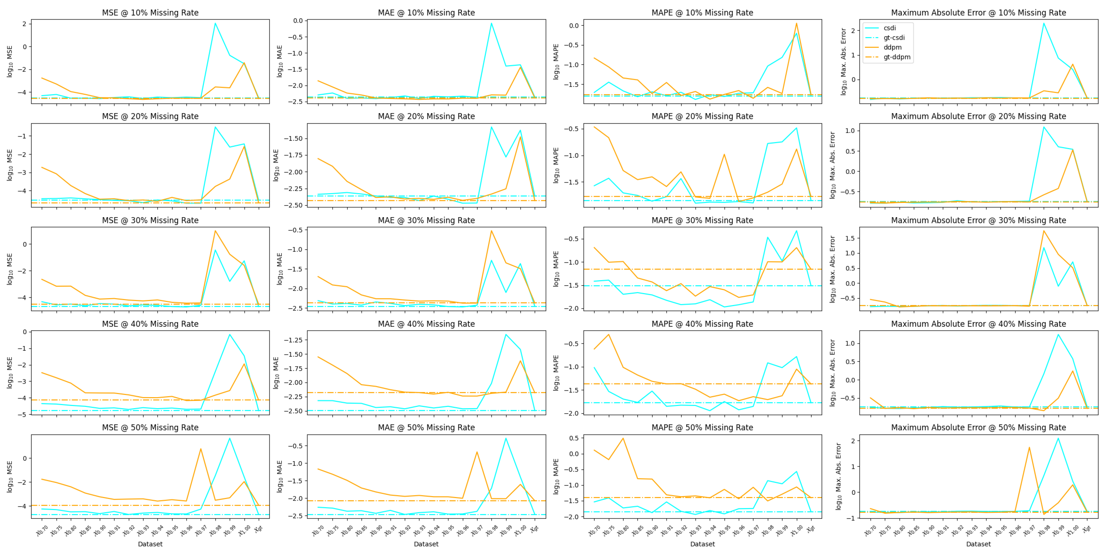
For each trained model we sample five estimates for each data-point in the dataset. We take the mean and standard deviation of each set of five samples and then fit a curve to the high confidence means with a standard deviation $<1$, using an SGF. We then take the mean squared, mean absolute, mean absolute percentage, and maximum absolute error of each fitted curve against a SGF fit of ${\mathcal{X}}_{gt}^n$.

Table A1. Training with missing ratio of $10\%$.

Dataset	Model	MAE	MAPE	MSE	Max.Abs.Err.
${\mathcal{X}}_{0.70}$	csdi	$5.04$ × 10−3	$1.94$ × 10−2	$4.71$ × 10−5	$3.06$ × 10−2
${\mathcal{X}}_{0.70}$	ddpm	$1.38$ × 10−2	$1.47$ × 10−1	$1.67$ × 10−3	$4.68$ × 10−1
${\mathcal{X}}_{0.75}$	csdi	$5.78$ × 10−3	$3.55$ × 10−2	$6.00$ × 10−5	$3.52$ × 10−2
${\mathcal{X}}_{0.75}$	ddpm	$8.90$ × 10−3	$8.67$ × 10−2	$4.99$ × 10−4	$2.68$ × 10−1
${\mathcal{X}}_{0.80}$	csdi	$3.96$ × 10−3	$2.12$ × 10−2	$2.83$ × 10−5	$3.11$ × 10−2
${\mathcal{X}}_{0.80}$	ddpm	$5.76$ × 10−3	$4.54$ × 10−2	$1.08$ × 10−4	$9.51$ × 10−2
${\mathcal{X}}_{0.85}$	csdi	$4.06$ × 10−3	$1.51$ × 10−2	$2.82$ × 10−5	$2.55$ × 10−2
${\mathcal{X}}_{0.85}$	ddpm	$5.02$ × 10−3	$4.05$ × 10−2	$6.09$ × 10−5	$5.75$ × 10−2
${\mathcal{X}}_{0.90}$	csdi	$3.89$ × 10−3	$2.02$ × 10−2	$2.61$ × 10−5	$3.46$ × 10−2
${\mathcal{X}}_{0.90}$	ddpm	$4.06$ × 10−3	$1.82$ × 10−2	$3.14$ × 10−5	$6.28$ × 10−2
${\mathcal{X}}_{0.91}$	csdi	$4.17$ × 10−3	$1.60$ × 10−2	$3.22$ × 10−5	$3.22$ × 10−2
${\mathcal{X}}_{0.91}$	ddpm	$3.92$ × 10−3	$3.48$ × 10−2	$3.02$ × 10−5	$4.55$ × 10−2
${\mathcal{X}}_{0.92}$	csdi	$4.69$ × 10−3	$1.96$ × 10−2	$3.73$ × 10−5	$3.17$ × 10−2
${\mathcal{X}}_{0.92}$	ddpm	$3.81$ × 10−3	$1.61$ × 10−2	$2.56$ × 10−5	$3.79$ × 10−2
${\mathcal{X}}_{0.93}$	csdi	$3.91$ × 10−3	$1.29$ × 10−2	$2.65$ × 10−5	$3.07$ × 10−2
${\mathcal{X}}_{0.93}$	ddpm	$3.66$ × 10−3	$2.05$ × 10−2	$2.20$ × 10−5	$2.78$ × 10−2
${\mathcal{X}}_{0.94}$	csdi	$4.56$ × 10−3	$1.70$ × 10−2	$3.53$ × 10−5	$3.20$ × 10−2
${\mathcal{X}}_{0.94}$	ddpm	$3.80$ × 10−3	$1.31$ × 10−2	$2.52$ × 10−5	$2.96$ × 10−2
${\mathcal{X}}_{0.95}$	csdi	$4.39$ × 10−3	$1.53$ × 10−2	$3.10$ × 10−5	$2.61$ × 10−2
${\mathcal{X}}_{0.95}$	ddpm	$3.79$ × 10−3	$1.73$ × 10−2	$2.86$ × 10−5	$5.43$ × 10−2
${\mathcal{X}}_{0.96}$	csdi	$4.62$ × 10−3	$1.85$ × 10−2	$3.51$ × 10−5	$2.51$ × 10−2
${\mathcal{X}}_{0.96}$	ddpm	$4.00$ × 10−3	$2.17$ × 10−2	$2.80$ × 10−5	$3.95$ × 10−2
${\mathcal{X}}_{0.97}$	csdi	$4.26$ × 10−3	$1.90$ × 10−2	$3.16$ × 10−5	$2.65$ × 10−2
${\mathcal{X}}_{0.97}$	ddpm	$3.97$ × 10−3	$1.38$ × 10−2	$2.79$ × 10−5	$3.52$ × 10−2
${\mathcal{X}}_{0.98}$	csdi	$8.30$ × 10−1	$9.13$ × 10−2	$1.11$ × 102	$1.94$ × 102
${\mathcal{X}}_{0.98}$	ddpm	$5.07$ × 10−3	$2.62$ × 10−2	$2.75$ × 10−4	$3.70$ × 10−1
${\mathcal{X}}_{0.99}$	csdi	$3.92$ × 10−2	$1.53$ × 10−1	$1.65$ × 10−1	$7.33$ × 100
${\mathcal{X}}_{0.99}$	ddpm	$4.98$ × 10−3	$1.83$ × 10−2	$2.31$ × 10−4	$3.05$ × 10−1
${\mathcal{X}}_{1.00}$	csdi	$4.29$ × 10−2	$6.27$ × 10−1	$3.01$ × 10−2	$2.87$ × 100
${\mathcal{X}}_{1.00}$	ddpm	$3.60$ × 10−2	$1.14$ × 100	$3.71$ × 10−2	$4.51$ × 100
${\mathcal{X}}_{GT}$	csdi	$4.31$ × 10−3	$1.58$ × 10−2	$3.11$ × 10−5	$3.01$ × 10−2
${\mathcal{X}}_{GT}$	ddpm	$4.07$ × 10−3	$1.72$ × 10−2	$2.62$ × 10−5	$2.19$ × 10−2

,

Table A2. Training with missing ratio of $20\%$.

Dataset	Model	MAE	MAPE	MSE	Max.Abs.Err.
${\mathcal{X}}_{0.70}$	csdi	$4.60$ × 10−3	$2.67$ × 10−2	$3.64$ × 10−5	$2.70$ × 10−2
${\mathcal{X}}_{0.70}$	ddpm	$1.57$ × 10−2	$3.43$ × 10−1	$1.89$ × 10−3	$5.21$ × 10−1
${\mathcal{X}}_{0.75}$	csdi	$4.71$ × 10−3	$3.70$ × 10−2	$3.74$ × 10−5	$3.12$ × 10−2
${\mathcal{X}}_{0.75}$	ddpm	$1.20$ × 10−2	$2.15$ × 10−1	$8.40$ × 10−4	$2.65$ × 10−1
${\mathcal{X}}_{0.80}$	csdi	$4.89$ × 10−3	$1.96$ × 10−2	$4.02$ × 10−5	$2.62$ × 10−2
${\mathcal{X}}_{0.80}$	ddpm	$7.18$ × 10−3	$5.17$ × 10−2	$1.91$ × 10−4	$1.35$ × 10−1
${\mathcal{X}}_{0.85}$	csdi	$4.65$ × 10−3	$1.76$ × 10−2	$3.60$ × 10−5	$3.50$ × 10−2
${\mathcal{X}}_{0.85}$	ddpm	$5.41$ × 10−3	$3.48$ × 10−2	$6.95$ × 10−5	$6.77$ × 10−2
${\mathcal{X}}_{0.90}$	csdi	$4.34$ × 10−3	$1.37$ × 10−2	$3.23$ × 10−5	$2.69$ × 10−2
${\mathcal{X}}_{0.90}$	ddpm	$4.12$ × 10−3	$3.93$ × 10−2	$3.41$ × 10−5	$5.77$ × 10−2
${\mathcal{X}}_{0.91}$	csdi	$4.13$ × 10−3	$1.66$ × 10−2	$2.95$ × 10−5	$3.49$ × 10−2
${\mathcal{X}}_{0.91}$	ddpm	$4.21$ × 10−3	$2.58$ × 10−2	$3.62$ × 10−5	$5.67$ × 10−2
${\mathcal{X}}_{0.92}$	csdi	$4.12$ × 10−3	$3.65$ × 10−2	$2.83$ × 10−5	$2.08$ × 10−2
${\mathcal{X}}_{0.92}$	ddpm	$3.91$ × 10−3	$4.89$ × 10−2	$2.86$ × 10−5	$5.47$ × 10−2
${\mathcal{X}}_{0.93}$	csdi	$3.70$ × 10−3	$1.25$ × 10−2	$2.22$ × 10−5	$2.66$ × 10−2
${\mathcal{X}}_{0.93}$	ddpm	$3.99$ × 10−3	$1.64$ × 10−2	$3.11$ × 10−5	$5.40$ × 10−2
${\mathcal{X}}_{0.94}$	csdi	$4.32$ × 10−3	$1.31$ × 10−2	$3.10$ × 10−5	$2.90$ × 10−2
${\mathcal{X}}_{0.94}$	ddpm	$3.87$ × 10−3	$1.55$ × 10−2	$2.63$ × 10−5	$4.38$ × 10−2
${\mathcal{X}}_{0.95}$	csdi	$3.88$ × 10−3	$1.30$ × 10−2	$2.78$ × 10−5	$3.02$ × 10−2
${\mathcal{X}}_{0.95}$	ddpm	$4.16$ × 10−3	$1.05$ × 10−1	$4.28$ × 10−5	$8.78$ × 10−2
${\mathcal{X}}_{0.96}$	csdi	$3.39$ × 10−3	$1.35$ × 10−2	$2.07$ × 10−5	$2.64$ × 10−2
${\mathcal{X}}_{0.96}$	ddpm	$3.73$ × 10−3	$1.34$ × 10−2	$2.87$ × 10−5	$6.32$ × 10−2
${\mathcal{X}}_{0.97}$	csdi	$3.40$ × 10−3	$1.27$ × 10−2	$2.07$ × 10−5	$3.73$ × 10−2
${\mathcal{X}}_{0.97}$	ddpm	$3.99$ × 10−3	$1.58$ × 10−2	$3.15$ × 10−5	$6.13$ × 10−2
${\mathcal{X}}_{0.98}$	csdi	$4.67$ × 10−2	$1.67$ × 10−1	$3.08$ × 10−1	$1.22$ × 101
${\mathcal{X}}_{0.98}$	ddpm	$4.64$ × 10−3	$2.02$ × 10−2	$1.71$ × 10−4	$2.85$ × 10−1
${\mathcal{X}}_{0.99}$	csdi	$1.66$ × 10−2	$1.79$ × 10−1	$2.43$ × 10−2	$3.93$ × 100
${\mathcal{X}}_{0.99}$	ddpm	$5.56$ × 10−3	$2.88$ × 10−2	$4.32$ × 10−4	$3.94$ × 10−1
${\mathcal{X}}_{1.00}$	csdi	$4.17$ × 10−2	$3.28$ × 10−1	$3.63$ × 10−2	$3.77$ × 100
${\mathcal{X}}_{1.00}$	ddpm	$3.32$ × 10−2	$1.31$ × 10−1	$2.60$ × 10−2	$3.66$ × 100
${\mathcal{X}}_{GT}$	csdi	$4.32$ × 10−3	$1.40$ × 10−2	$3.13$ × 10−5	$2.32$ × 10−2
${\mathcal{X}}_{GT}$	ddpm	$3.69$ × 10−3	$1.68$ × 10−2	$2.19$ × 10−5	$2.18$ × 10−2

,

Table A3. Training with missing ratio of $30\%$.

Dataset	Model	MAE	MAPE	MSE	Max.Abs.Err.
${\mathcal{X}}_{0.70}$	csdi	$4.85$ × 10−3	$3.84$ × 10−2	$4.70$ × 10−5	$4.77$ × 10−2
${\mathcal{X}}_{0.70}$	ddpm	$2.01$ × 10−2	$2.04$ × 10−1	$2.22$ × 10−3	$4.06$ × 10−1
${\mathcal{X}}_{0.75}$	csdi	$3.98$ × 10−3	$4.05$ × 10−2	$2.70$ × 10−5	$2.52$ × 10−2
${\mathcal{X}}_{0.75}$	ddpm	$1.23$ × 10−2	$9.85$ × 10−2	$6.79$ × 10−4	$2.17$ × 10−1
${\mathcal{X}}_{0.80}$	csdi	$4.11$ × 10−3	$2.01$ × 10−2	$3.13$ × 10−5	$3.37$ × 10−2
${\mathcal{X}}_{0.80}$	ddpm	$1.10$ × 10−2	$1.02$ × 10−1	$6.89$ × 10−4	$3.86$ × 10−1
${\mathcal{X}}_{0.85}$	csdi	$3.73$ × 10−3	$2.18$ × 10−2	$2.34$ × 10−5	$2.36$ × 10−2
${\mathcal{X}}_{0.85}$	ddpm	$6.81$ × 10−3	$4.51$ × 10−2	$1.40$ × 10−4	$1.64$ × 10−1
${\mathcal{X}}_{0.90}$	csdi	$4.51$ × 10−3	$1.94$ × 10−2	$3.39$ × 10−5	$2.55$ × 10−2
${\mathcal{X}}_{0.90}$	ddpm	$5.44$ × 10−3	$3.70$ × 10−2	$7.38$ × 10−5	$1.19$ × 10−1
${\mathcal{X}}_{0.91}$	csdi	$4.14$ × 10−3	$1.49$ × 10−2	$3.11$ × 10−5	$2.40$ × 10−2
${\mathcal{X}}_{0.91}$	ddpm	$5.44$ × 10−3	$2.40$ × 10−2	$8.15$ × 10−5	$1.10$ × 10−1
${\mathcal{X}}_{0.92}$	csdi	$3.62$ × 10−3	$1.20$ × 10−2	$2.28$ × 10−5	$2.82$ × 10−2
${\mathcal{X}}_{0.92}$	ddpm	$5.04$ × 10−3	$3.41$ × 10−2	$6.21$ × 10−5	$9.73$ × 10−2
${\mathcal{X}}_{0.93}$	csdi	$3.92$ × 10−3	$1.25$ × 10−2	$2.70$ × 10−5	$2.75$ × 10−2
${\mathcal{X}}_{0.93}$	ddpm	$4.73$ × 10−3	$1.83$ × 10−2	$5.37$ × 10−5	$1.08$ × 10−1
${\mathcal{X}}_{0.94}$	csdi	$3.79$ × 10−3	$1.53$ × 10−2	$2.49$ × 10−5	$2.97$ × 10−2
${\mathcal{X}}_{0.94}$	ddpm	$4.81$ × 10−3	$2.94$ × 10−2	$6.37$ × 10−5	$1.06$ × 10−1
${\mathcal{X}}_{0.95}$	csdi	$3.43$ × 10−3	$1.07$ × 10−2	$2.03$ × 10−5	$3.10$ × 10−2
${\mathcal{X}}_{0.95}$	ddpm	$4.74$ × 10−3	$2.51$ × 10−2	$4.23$ × 10−5	$5.65$ × 10−2
${\mathcal{X}}_{0.96}$	csdi	$3.36$ × 10−3	$1.19$ × 10−2	$1.91$ × 10−5	$2.67$ × 10−2
${\mathcal{X}}_{0.96}$	ddpm	$4.20$ × 10−3	$1.72$ × 10−2	$3.66$ × 10−5	$7.12$ × 10−2
${\mathcal{X}}_{0.97}$	csdi	$3.71$ × 10−3	$1.37$ × 10−2	$2.50$ × 10−5	$3.52$ × 10−2
${\mathcal{X}}_{0.97}$	ddpm	$4.21$ × 10−3	$1.95$ × 10−2	$3.81$ × 10−5	$7.50$ × 10−2
${\mathcal{X}}_{0.98}$	csdi	$5.24$ × 10−2	$3.40$ × 10−1	$3.51$ × 10−1	$1.51$ × 101
${\mathcal{X}}_{0.98}$	ddpm	$3.01$ × 10−1	$1.01$ × 10−1	$9.83$ × 100	$5.54$ × 101
${\mathcal{X}}_{0.99}$	csdi	$7.87$ × 10−3	$1.05$ × 10−1	$1.57$ × 10−3	$7.01$ × 10−1
${\mathcal{X}}_{0.99}$	ddpm	$4.51$ × 10−2	$1.00$ × 10−1	$1.68$ × 10−1	$9.09$ × 100
${\mathcal{X}}_{1.00}$	csdi	$4.32$ × 10−2	$4.72$ × 10−1	$5.42$ × 10−2	$5.40$ × 100
${\mathcal{X}}_{1.00}$	ddpm	$3.21$ × 10−2	$2.03$ × 10−1	$2.47$ × 10−2	$3.55$ × 100
${\mathcal{X}}_{GT}$	csdi	$3.48$ × 10−3	$3.08$ × 10−2	$2.02$ × 10−5	$2.44$ × 10−2
${\mathcal{X}}_{GT}$	ddpm	$4.22$ × 10−3	$6.94$ × 10−2	$3.03$ × 10−5	$3.76$ × 10−2

,

Table A4. Training with missing ratio of $40\%$.

Dataset	Model	MAE	MAPE	MSE	Max.Abs.Err.
${\mathcal{X}}_{0.70}$	csdi	$4.78$ × 10−3	$9.55$ × 10−2	$4.45$ × 10−5	$3.28$ × 10−2
${\mathcal{X}}_{0.70}$	ddpm	$2.81$ × 10−2	$2.40$ × 10−1	$3.31$ × 10−3	$4.80$ × 10−1
${\mathcal{X}}_{0.75}$	csdi	$4.77$ × 10−3	$2.93$ × 10−2	$4.19$ × 10−5	$3.18$ × 10−2
${\mathcal{X}}_{0.75}$	ddpm	$2.02$ × 10−2	$4.94$ × 10−1	$1.64$ × 10−3	$3.66$ × 10−1
${\mathcal{X}}_{0.80}$	csdi	$4.33$ × 10−3	$2.01$ × 10−2	$3.49$ × 10−5	$3.07$ × 10−2
${\mathcal{X}}_{0.80}$	ddpm	$1.43$ × 10−2	$9.67$ × 10−2	$7.76$ × 10−4	$3.56$ × 10−1
${\mathcal{X}}_{0.85}$	csdi	$4.28$ × 10−3	$1.70$ × 10−2	$3.07$ × 10−5	$2.41$ × 10−2
${\mathcal{X}}_{0.85}$	ddpm	$9.11$ × 10−3	$6.59$ × 10−2	$2.01$ × 10−4	$1.41$ × 10−1
${\mathcal{X}}_{0.90}$	csdi	$3.61$ × 10−3	$2.98$ × 10−2	$2.30$ × 10−5	$2.37$ × 10−2
${\mathcal{X}}_{0.90}$	ddpm	$8.51$ × 10−3	$4.84$ × 10−2	$1.97$ × 10−4	$1.78$ × 10−1
${\mathcal{X}}_{0.91}$	csdi	$3.73$ × 10−3	$1.40$ × 10−2	$2.47$ × 10−5	$2.62$ × 10−2
${\mathcal{X}}_{0.91}$	ddpm	$7.44$ × 10−3	$4.25$ × 10−2	$1.94$ × 10−4	$2.13$ × 10−1
${\mathcal{X}}_{0.92}$	csdi	$3.43$ × 10−3	$1.48$ × 10−2	$1.98$ × 10−5	$2.17$ × 10−2
${\mathcal{X}}_{0.92}$	ddpm	$6.74$ × 10−3	$4.30$ × 10−2	$1.51$ × 10−4	$2.24$ × 10−1
${\mathcal{X}}_{0.93}$	csdi	$3.87$ × 10−3	$1.46$ × 10−2	$2.55$ × 10−5	$2.31$ × 10−2
${\mathcal{X}}_{0.93}$	ddpm	$6.62$ × 10−3	$3.27$ × 10−2	$1.03$ × 10−4	$1.10$ × 10−1
${\mathcal{X}}_{0.94}$	csdi	$3.55$ × 10−3	$1.13$ × 10−2	$2.20$ × 10−5	$2.66$ × 10−2
${\mathcal{X}}_{0.94}$	ddpm	$6.23$ × 10−3	$2.20$ × 10−2	$1.02$ × 10−4	$1.15$ × 10−1
${\mathcal{X}}_{0.95}$	csdi	$3.80$ × 10−3	$1.77$ × 10−2	$2.41$ × 10−5	$2.83$ × 10−2
${\mathcal{X}}_{0.95}$	ddpm	$6.70$ × 10−3	$2.56$ × 10−2	$1.22$ × 10−4	$1.39$ × 10−1
${\mathcal{X}}_{0.96}$	csdi	$3.43$ × 10−3	$1.18$ × 10−2	$2.02$ × 10−5	$2.57$ × 10−2
${\mathcal{X}}_{0.96}$	ddpm	$5.75$ × 10−3	$1.85$ × 10−2	$6.82$ × 10−5	$7.44$ × 10−2
${\mathcal{X}}_{0.97}$	csdi	$3.46$ × 10−3	$1.40$ × 10−2	$2.09$ × 10−5	$3.24$ × 10−2
${\mathcal{X}}_{0.97}$	ddpm	$5.74$ × 10−3	$2.26$ × 10−2	$7.12$ × 10−5	$9.69$ × 10−2
${\mathcal{X}}_{0.98}$	csdi	$9.62$ × 10−3	$1.21$ × 10−1	$3.89$ × 10−3	$1.33$ × 100
${\mathcal{X}}_{0.98}$	ddpm	$6.42$ × 10−3	$1.95$ × 10−2	$1.45$ × 10−4	$1.69$ × 10−1
${\mathcal{X}}_{0.99}$	csdi	$6.97$ × 10−2	$9.52$ × 10−2	$6.84$ × 10−1	$1.73$ × 101
${\mathcal{X}}_{0.99}$	ddpm	$6.75$ × 10−3	$2.36$ × 10−2	$2.75$ × 10−4	$3.32$ × 10−1
${\mathcal{X}}_{1.00}$	csdi	$3.80$ × 10−2	$1.65$ × 10−1	$3.46$ × 10−2	$4.06$ × 100
${\mathcal{X}}_{1.00}$	ddpm	$2.40$ × 10−2	$8.85$ × 10−2	$1.13$ × 10−2	$2.05$ × 100
${\mathcal{X}}_{GT}$	csdi	$3.18$ × 10−3	$1.67$ × 10−2	$1.67$ × 10−5	$2.22$ × 10−2
${\mathcal{X}}_{GT}$	ddpm	$6.58$ × 10−3	$4.23$ × 10−2	$7.30$ × 10−5	$5.85$ × 10−2

and

Table A5. Training with missing ratio of $50\%$.

Dataset	Model	MAE	MAPE	MSE	Max.Abs.Err.
${\mathcal{X}}_{0.70}$	csdi	$5.45$ × 10−3	$2.91$ × 10−2	$5.50$ × 10−5	$4.39$ × 10−2
${\mathcal{X}}_{0.70}$	ddpm	$6.76$ × 10−2	$1.29$ × 100	$1.69$ × 10−2	$8.06$ × 10−1
${\mathcal{X}}_{0.75}$	csdi	$5.15$ × 10−3	$3.92$ × 10−2	$4.83$ × 10−5	$3.21$ × 10−2
${\mathcal{X}}_{0.75}$	ddpm	$4.79$ × 10−2	$6.44$ × 10−1	$8.94$ × 10−3	$6.32$ × 10−1
${\mathcal{X}}_{0.80}$	csdi	$4.20$ × 10−3	$1.87$ × 10−2	$3.16$ × 10−5	$3.39$ × 10−2
${\mathcal{X}}_{0.80}$	ddpm	$3.21$ × 10−2	$3.10$ × 100	$3.93$ × 10−3	$4.82$ × 10−1
${\mathcal{X}}_{0.85}$	csdi	$4.34$ × 10−3	$2.11$ × 10−2	$3.28$ × 10−5	$2.66$ × 10−2
${\mathcal{X}}_{0.85}$	ddpm	$1.94$ × 10−2	$1.59$ × 10−1	$1.18$ × 10−3	$4.16$ × 10−1
${\mathcal{X}}_{0.90}$	csdi	$3.66$ × 10−3	$1.32$ × 10−2	$2.24$ × 10−5	$2.73$ × 10−2
${\mathcal{X}}_{0.90}$	ddpm	$1.49$ × 10−2	$1.55$ × 10−1	$5.74$ × 10−4	$1.76$ × 10−1
${\mathcal{X}}_{0.91}$	csdi	$4.44$ × 10−3	$2.90$ × 10−2	$3.39$ × 10−5	$3.41$ × 10−2
${\mathcal{X}}_{0.91}$	ddpm	$1.22$ × 10−2	$4.88$ × 10−2	$3.48$ × 10−4	$2.10$ × 10−1
${\mathcal{X}}_{0.92}$	csdi	$3.40$ × 10−3	$1.46$ × 10−2	$1.92$ × 10−5	$3.22$ × 10−2
${\mathcal{X}}_{0.92}$	ddpm	$1.12$ × 10−2	$4.24$ × 10−2	$3.70$ × 10−4	$2.70$ × 10−1
${\mathcal{X}}_{0.93}$	csdi	$3.82$ × 10−3	$1.16$ × 10−2	$2.49$ × 10−5	$2.55$ × 10−2
${\mathcal{X}}_{0.93}$	ddpm	$1.19$ × 10−2	$4.52$ × 10−2	$3.88$ × 10−4	$2.74$ × 10−1
${\mathcal{X}}_{0.94}$	csdi	$4.04$ × 10−3	$1.54$ × 10−2	$2.83$ × 10−5	$2.68$ × 10−2
${\mathcal{X}}_{0.94}$	ddpm	$1.09$ × 10−2	$3.92$ × 10−2	$2.51$ × 10−4	$1.33$ × 10−1
${\mathcal{X}}_{0.95}$	csdi	$3.48$ × 10−3	$1.21$ × 10−2	$2.15$ × 10−5	$3.75$ × 10−2
${\mathcal{X}}_{0.95}$	ddpm	$1.08$ × 10−2	$7.26$ × 10−2	$3.28$ × 10−4	$2.67$ × 10−1
${\mathcal{X}}_{0.96}$	csdi	$3.51$ × 10−3	$1.76$ × 10−2	$2.11$ × 10−5	$2.23$ × 10−2
${\mathcal{X}}_{0.96}$	ddpm	$9.84$ × 10−3	$3.66$ × 10−2	$2.55$ × 10−4	$1.89$ × 10−1
${\mathcal{X}}_{0.97}$	csdi	$4.17$ × 10−3	$1.79$ × 10−2	$5.38$ × 10−5	$1.35$ × 10−1
${\mathcal{X}}_{0.97}$	ddpm	$2.08$ × 10−1	$8.47$ × 10−2	$5.98$ × 100	$5.54$ × 101
${\mathcal{X}}_{0.98}$	csdi	$1.90$ × 10−2	$1.38$ × 10−1	$3.37$ × 10−2	$4.45$ × 100
${\mathcal{X}}_{0.98}$	ddpm	$9.61$ × 10−3	$3.12$ × 10−2	$2.97$ × 10−4	$2.77$ × 10−1
${\mathcal{X}}_{0.99}$	csdi	$5.13$ × 10−1	$1.10$ × 10−1	$4.54$ × 101	$1.25$ × 102
${\mathcal{X}}_{0.99}$	ddpm	$9.58$ × 10−3	$5.11$ × 10−2	$4.75$ × 10−4	$4.05$ × 10−1
${\mathcal{X}}_{1.00}$	csdi	$3.99$ × 10−2	$2.70$ × 10−1	$2.62$ × 10−2	$2.98$ × 100
${\mathcal{X}}_{1.00}$	ddpm	$2.45$ × 10−2	$8.68$ × 10−2	$1.07$ × 10−2	$2.24$ × 100
${\mathcal{X}}_{GT}$	csdi	$3.40$ × 10−3	$1.42$ × 10−2	$1.94$ × 10−5	$2.38$ × 10−2
${\mathcal{X}}_{GT}$	ddpm	$8.34$ × 10−3	$3.96$ × 10−2	$1.13$ × 10−4	$5.17$ × 10−2

in Appendix A tabulate the results of a series the experiments conducted as described above; results are also summarized in the series of plots given in Figure 3. The plots in Figure 3 reveal consistent dynamics related to the training of the models over the datasets. In general, the CSDI models outperform their DDPM counterparts and achieve the best performance in each error category with the exception of maximum absolute error. The hatched constant vertical lines in the plots of Figure 3 show the performance of the models when trained on the ground truth dataset ${\mathcal{X}}_{gt}$. Although there are some exceptions, generally, models trained on the ground truth dataset out-perform their counterparts trained on the MSE threshold based datasets; this suggests that models trained on the ground truth datasets are indeed learning ∼$P\left(x_{gt}^n\right|{\mathcal{X}}_{gt}^n)$, while those trained on datasets whose partitions mix data from nominal and anomalous data generating factors are learning some other similar but different distributions. Further, we posit that when model performance on an arbitrary MSE dataset ${\mathcal{X}}_{\kappa }$ meets or exceeds the performance of the same model when trained on ${\mathcal{X}}_{gt}$, then it is likely that the distribution learned by the model, presumably ∼$P\left(x_{\kappa }^n\right|{\mathcal{X}}_{\kappa }^n)$, is in some meaningful way similar to the distribution learned by the model trained on ground truth—presumably $P\left(x_{gt}^n\right|{\mathcal{X}}_{gt}^n)$. This line of thinking suggests that the NDM and ODM, in so far as they are able to predict aspects of implemented neural network performance, provide some measure of explainability to results. In a practical setting this explainability, in conjunction with quantitative targets for error, can be leveraged to generate confidence that a model has achieved a satisfactory level of performance, and allows regulators to understand the basis for results.

A consistent feature of the plots in Figure 3 is a spike in error rates somewhere above the 96th MSE percentile. Figure 4 may explain this by providing insight into the quality of the data being added to the nominal population at the high MSE threshold range. It is at just above the 96th MSE percentile that the qualitative nature of the intersection population growth curves changes. We note that at the lower range of threshold values, changes in intersection membership occur in large steps. At the upper range of threshold values, the change in membership occurs more smoothly. This speaks directly to the uniqueness, or alternatively to the amount of information, in the data being added to the intersection. As per information theory, the more unique a datum, the more information it carries relative to the data. So, we observe that as intersection set membership additions become increasingly unique, the model error in Figure 3 increases dramatically. This suggests that the trend of the highly informative data are not as easily encoded as the more common low MSE data in the weights of the neural networks implementing the DPM.

From the perspective of the CSDI conditional loss function, the information content of the unique outliers is largely irrelevant. An outlying time of flight has very little information to relate about the largely continuous nominal signal in and around which it occurs. More over with their high information content the outliers are likely to generate some number of spurious correlations with the rest of the dataset. So the conditional CSDI model struggles, colloquially in two directions, to make sense of the highly informative anomalous information. Conversely, when on average there is less information per element in the nominal partition the CSDI model is enabled to learn the possibly continuous, possibly well-defined structure of the data. In the case of a highly structured dataset, each element bears a strong, identifiable, possibly causal conditional relation to neighboring data. CSDI leverages this conditional structure and given a largely nominal signal in the dataset readily learns the nominal distribution. DDPM models do not take advantage of this conditional perspective on the nominal information and, as borne out in the results, are slightly impaired in learning the nominal distribution. DDPM models are also more tolerant of outliers when they occur. This is directly observed in Figure 3 where at thresholds less than the 96th MSE percentile CSDI models generally outperform DDPM models, but in the range above the 96th, their error ramps up quickly and often exceeds that of DDPM models.

Figure 5 show the results of a second set of experiments where we test the effect of enlarging a dataset with predominantly nominal signal. This drives the ratio of the nominal to total population in each dataset towards unity. This tests and affirms the assumption that ${lim}_{\frac{|{\mathcal{X}}^n|}{\left|\mathcal{X}\right|}\to 1}P\left(x\right|\mathcal{X})=P\left(x^n\right|{\mathcal{X}}^n)$. We observe that as the dataset size increases MAE error improves across the range of datasets. We also observe that the range of error increases so that over and above the 96th percentile error ramps up more quickly as dataset size enlarges. This is suggests that as training becomes saturated by the nominal signal in the dataset the loss function naturally encodes information in the neural network weights that secure the most numerical benefit. This in turn causes error to become increasingly sensitive to anomalous data.

9. Practical Application and Future Work

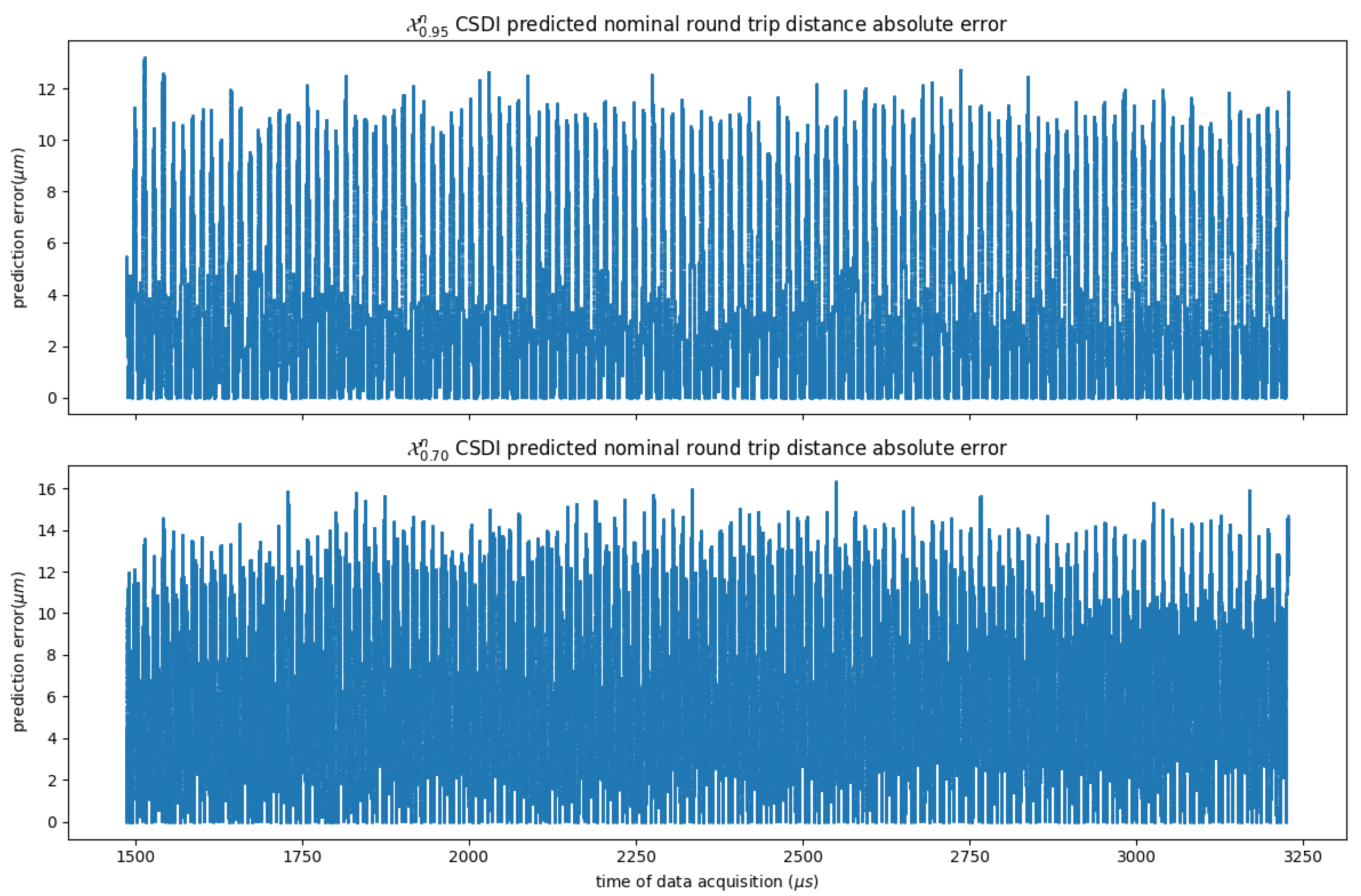
Figure 6 gives the error in microns ($\mathsf{\mu }$m) against ground truth, for estimates of peak amplitude time of flight as provided by CSDI models trained on ${\mathcal{X}}_{0.95}$ and ${\mathcal{X}}_{0.70}$ partitioned datasets. For the UT NDE inspection of nuclear CANDU PT, the minimum deviation from nominal that must be reported is 100 $\mathsf{\mu }$m. In practice, the minimum reportable deviation sits at the edge of human cognitive abilities, and for anomalies in this range the data are often unclear, which causes analysis to be somewhat subjective. To support this point of view we note that, in the best conditions, subject matter experts consider the accuracy of manual analysis to be within a 40 $\mathsf{\mu }$m band. This suggests that the CSDI-based estimates are at least on par with manual analysis. To be sure, a further study and quantification of the delta between model-based estimates and manual analysis in the low range <100 $\mathsf{\mu }$m is required.

In-the-field usage of DPM-based estimates would require some means for fault diagnosis without reference to ground truth. There are numerous avenues for engineering solutions that involve the use of agreement between multiple independent estimation techniques. One opportunity for a second estimation technique, currently being investigated, involves the use of a dynamic nominal partition that changes in response to a self-supervised signal provided during training. Though this may improve the robustness of results, without ground truth we see no opportunity to provide concrete guarantees on model performance. Given that this is the case, we think it likely that automation and decision support for UT NDE data analysis will necessarily involve a human in the loop, driving an iterative process of training, verification, and reclassification. So for instance, a practical procedure might assign a well chosen partition to a UT NDE dataset and train a model on it, and after sampling allow an analyst to verify the classification of data in regions where the sampled estimates vary, beyond some bound, from observed data. The analyst might then tweak the partition and retrain the model to achieve superior results. This process of training and directed manual reclassification would continue, until some quantifiable error objective was achieved; this process would almost surely force the nominal partition in the direction of ground truth and ensure satisfactory performance across the dataset.

A number of opportunities exist for improving results. Figure 7 shows in detail the fit of CSDI estimates, as well as the support of ${\mathcal{X}}_{0.95}^n$ on which the model was trained. What is clear is that the SGF fit on estimates overshoots the weight of the data in and around regions where its derivative is close to zero. This wig wag could in part be due to the Gaussian prior distribution used by CSDI models, and could also in part be due to the nature of SGF curve fitting. A post-processing step that introduced weight to the SGF from observed data in and around the neighborhood of estimates might serve to ameliorate the wig wag. A slightly more involved improvement might involve the use of alternative priors, with more degrees of freedom than the Gaussian, in the diffusion process [23].

One area of concern is the degree of support from nominal data on which estimates are based. Typically, inspection processes have some data quality argument attached to them that specifies the minimum level of support from observed data on which an estimate must be based. We pay attention, in Figure 7, to the shaded gray region of the scatter plot showing the set membership in ${\mathcal{X}}_{0.95}^n$ on which CSDI estimates are based. There we see that the partition selected by the 95th MSE percentile discriminates against likely nominal observed data, and places it in ${\mathcal{X}}_{0.95}^a$. Although the estimates are of high quality, it would be better, from a process quality point of view, to include the discriminated data in the nominal set. Again an iterative process with a human in the loop could include tools that identify regions of low support, allow for suitable data reclassification, and then retraining.

10. Conclusions

We model the UT NDE data analysis task probabilistically as the NDM and ODM and evaluate the potential to provide decision support and automation to UT NDE data analysis using their CSDI- and DDPM-based implementations. We demonstrate the veracity and utility of the NDM and ODM by way of their ability to explain the variance in CSDI and DDPM performance across a variety of uniquely partitioned UT NDE datasets. We show that the NDM and ODM provide a basis for understanding the behavior of their CSDI and DDPM based implementations. And thus provide a basis for a technical justification needed to support the use of diffusion based methods in safety critical contexts in practice.

We train the CSDI model on various datasets to learn the NDM and sample from it to obtain estimates of peak amplitude response time of flight. We sample estimates from trained CSDI models and find their accuracy, against ground truth, to be on par with manual analysis. The unsupervised training procedure does not rely on dataset labelling or annotation, and the accuracy of sampled estimates depends only on learning the distribution of a single dataset. In this way, the approach may be used offline on a per-inspection basis, with no data annotation, and without recourse to out of distribution generalization. We suggest various means to improve results and confidence therein. We also suggest an iterative human-in-the-loop training verification process that may act, in lieu of the availability of ground truth, as a means for fault detection and remediation.

The method improves greatly upon prior work where results rely on data annotation, pre-processing, brittle heuristics, and out-of-distribution generalization. And the probabilistic model-based explainability provides a basis for interface with regulatory bodies seeking some justification for usage of novel methods in safety-critical contexts.