Simulation of Calibrated Complex Synthetic Population Data with XGBoost

Abstract

Syntheticdata generation methods are used to transform the original data into privacy-compliant synthetic copies (twin data). With our proposed approach, synthetic data can be simulated in the same size as the input data or in any size, and in the case of finite populations, even the entire population can be simulated. The proposed XGBoost-based method is compared with known model-based approaches to generate synthetic data using a complex survey data set. The XGBoost method shows strong performance, especially with synthetic categorical variables, and outperforms other tested methods. Furthermore, the structure and relationship between variables are well preserved. The tuning of the parameters is performed automatically by a modified k-fold cross-validation. If exact population margins are known, e.g., cross-tabulated population counts on age class, gender and region, the synthetic data must be calibrated to those known population margins. For this purpose, we have implemented a simulated annealing algorithm that is able to use multiple population margins simultaneously to post-calibrate a synthetic population. The algorithm is, thus, able to calibrate simulated population data containing cluster and individual information, e.g., about persons in households, at both person and household level. Furthermore, the algorithm is efficiently implemented so that the adjustment of populations with many millions or more persons is possible.

1. Introduction

The generation of synthetic data is one way to comply with general data protection laws [1]. However, this is not the only way to solve the problem of confidentiality. Data can be shared in different forms. In traditional anonymization, data are anonymized under the paradigm of high data utility to create scientific or public use files. In this process, the data are altered so that the risk of disclosure to individuals falls below a certain threshold, under the condition that the data are as useful as possible. Remote execution, secure labs and remote access are other data-sharing options (with synthetic data required for remote execution). Query servers deal with perturbed aggregated results using differential privacy [2], secondary cell suppression [3], or the cellKey method [4] or target record swapping (see, e.g., [5]). Black-box methods for obtaining predictions on test data are a way to share not data but predictions on single sensitive variables without having access to training data. Typically, this is used in a federated learning environment where data sources are not centralized but distributed across multiple peers [6].

Synthetic data avoid the costly remote access and federated learning approaches and are an attractive and well-established alternative to the aforementioned approaches.

1.1. Synthetic Data

Synthetic data are used as training data in machine learning, for augmented data or in the form of population data, and as twin data for the public or for sharing within an organization to speed things up so that data can already be used before administrative issues regarding data access are solved. Instead of introducing changes in the original data, central structures of the data and relationships between variables are used to generate new data. The methods for creating synthetic data stem from the machine learning (ML), AI and statistical modeling domains. They learn the parameters of the models on the original data and use them to generate artificial data. Synthetic data are associated with low disclosure risk [7,8,9] and advantages in the simplicity of the process—once synthetic data are generated.

Synthetic data have surged in popularity and are now utilized across a myriad of scenarios where real-world data were traditionally employed. They offer a cost-effective and hassle-free testing environment that can subsequently be verified with real-world data. This shift underscores the significant role that synthetic data play in modern data analytics. This applies to various research areas. For instance, a commonly used synthetic data set in the literature are the synthetic data of the European Statistics on Income and Living Conditions (EU-SILC), created by [10], or the synthetic version of the Structure of Earnings Survey [11], both conducted in all member states of the European Union (as well as some other countries, such as Switzerland).

The basic motivation to create synthetic data is either to compare methods in simulation studies or to find a way to share confidential data. For both, the quality of synthetic data is crucial, and the synthetic data need to reflect the properties of real data.

But what is meant by close-to-reality/realistic data? (see, similarly, also [12])

-

Socio-demographic-economic structure of persons and strata need to be reflected.

-

Marginal distributions and interactions between variables should be represented correctly.

-

Hierarchical and cluster structures have to be preserved.

-

Certain marginal distributions must exactly match known values.

-

Data confidentiality must be ensured; thus, replication of units (e.g., using a bootstrap approach) should be avoided.

1.2. Synthetic Populations

Simulating not only a sample survey but the entire population has some advantages. For example, in agent-based and/or micro-simulation approaches, information about individuals in the whole population is needed. For example, to simulate the epidemic spread of COVID-19 under certain conditions in a micro-simulation environment, socioeconomic and health information is needed on all individuals at a given time.

Note that if only a synthetic sample survey is required, it can be drawn from the synthetic population using a realistic sampling plan. In this way, the creation of the whole population is richer in application and more general.

Software for synthetic data simulation in R is, for example, provided by synthpop [13] for data without any of the mentioned complicated structures (e.g., persons in households) and surveys obtained with simple random sampling. simPop [14] is the only software that considers complex data sets to allow hierarchical and cluster structures and samples from complex survey designs, including sampling weights from complex sampling procedures. Realistic cluster structures are important, e.g., not to create households with only children or an 80-year-old mother with a young son, to give some simplified illustrative examples. simPop additionally allows for population simulation.

1.3. Non-Linear Synthesizers

Recently, non-linear methods from artificial neural networks have also been used to synthesize data, for example, using generative additive networks (GAN) [15] as a joint modeling approach. Clearly, using deep learning methods to learn all relationships, e.g., that a household cannot consist only of children or more complicated logical conditions, is often not possible and parameter tuning must be performed with great care. Also joint modeling of all variables in a data set is naturally only visible for a small number of variables, and it is quite obvious that, e.g., when applying a joint modeling approach (e.g., with GAN), it becomes too noisy with a high number of variables, e.g., when simulating a complex data set with 25 variables or more. This is also naturally true for LLMs used for synthetic data generation as, e.g., in [16].

Therefore, fully conditional modeling approaches come into play, where variables are simulated sequentially. A type of non-linear method that uses a fully conditional modeling approach and which is well implemented in software (e.g., in the R packages synthpop [13] and simPop) is random forest adapted to synthesize variables in a data set.

1.4. Calibration

One should not stop at having synthetic twin data sets simulated with a synthesizer, but additionally modify the synthetic data so that certain marginal sums match the original data set and/or known characteristics of the population. To give an illustrative example. Imagine a user calculating the total number of 45–50-year-old men and women for each region. He would be confused if the results from the synthetic data differed (even slightly) from the official figures from the national agency. Therefore, some marginal totals have to be estimated accurately with synthetic data, and synthetic data have to be calibrated to known population characteristics.

Calibration should always be used when auxiliary information is available [17], not only for the consistency named before, but also for the reason of using all available information that improves the synthetic data. In general, it can be said that there is no calibration approach if no auxiliary information is available, since there is nothing to calibrate against. In the case of synthetic data, either population characteristics are known from administrative data, or/and characteristics such as marginal totals are known from the original data. Calibration can, therefore, be used to adjust the synthetic population to the known external population totals.

In R, there is a lot of software for calculating calibration weights, e.g., the packages survey and surveysd are two of them. These weights are calibrated using auxiliary information from administrative registers, other accurate sources, or even original data sets. However, with these tools and methods, it is not possible to calibrate synthetic populations.

1.5. Calibration of Populations

The previously weight-based approaches cannot be used for synthetic populations because the selection probability of each individual in the population is 1 and, therefore, the weights should be 1. The recalibration step presented in this paper is a combinatorial optimization problem with the aim of drawing clusters (such as households) from the synthetic population (of individuals) in such a way that the difference between the margins from selection and a given set of population margins is minimized and substantially extends existing methods. In this way, the cluster information is preserved while the margins are respected.

In practice, it is a typical situation that auxiliary information is available not only for persons but also for households or enterprises (employers) and also for employees, etc. In this case, several different types of multiple margins are known, and these margins are defined for different types of units in a data set.

1.6. Outline

The framework and workflow are illustrated in Figure 1. Essentially, the framework comprises three steps, with the second and third steps introducing new contributions to literature and software. The three items below match the numbers in Figure 1.

Figure 1. The workflow to produce a synthetic population and to calibrate it. The contribution covers the large light blue area together with the synthesis step 2 using XGBoost. The corresponding text passages are linked to section numbers in the Figure.

• The synthetic hierarchical structure is simulated, e.g., age and gender of persons in households.
• Synthetic data simulation with XGBoost to simulate synthetic population data with (possible) complex structures (like persons in households) from complex samples with (possible) complex sampling plans.
• Calibration of the simulated population to known margins with a new calibration technique that allows multiple margins for different information (e.g., household information and personal information simultaneously).

All these steps might be needed to simulate realistic synthetic populations, and we show the benefits of these new developments.

The remainder of the essential parts of the article is structured as follows.

-

In Section 2.3, the well-known XGBoost method is introduced in a general manner. After this short introduction, the simulation of the synthetic population is shown.

-

The first aim is to create a synthetic structural file (Section 2.2, cf. Figure 1, first point) that includes the cluster information.

-

Using the information of the non-anonymized data and the synthetic hierarchical/cluster structure, the remaining variables can now be simulated using XGBoost (cf. Figure 1, second point). While random forests build their regression trees independently (for each variable to be simulated), XGBoost improves the selection of trees at each step. XGBoost thus generally combines two important aspects: non-linear adjustments and improvements (due to a loss function) in each selected tree. The adaption of XGBoost to be used to simulate synthetic variables is described in Section 2.3.3 and the information used is visible in Figure 1. The cross-validation procedure to determine the hyperparameters in XGBoost is also reported in Section 2.3.4. After simulation of the synthetic population (see Figure 1, third step), the quality of the simulated data is discussed in Section 2.4.

-

Section 3 then shows how the simulated population can be calibrated to known multiple population margins (e.g., margins on households and information on persons in Section 3.2) considering the cluster structure in the data. Several subsections (Section 3.3, Section 3.4 and Section 3.5) are dedicated to this problem. Note that the draft version of this calibration method was already implemented in the R package simPop but has never been published in a scientific journal, and we have considerably extended the methods within this contribution.

-

Section 3.6 shows the impact of calibration on several statistics.

-

Section 4 discusses the implications of these methods for applications and science.

-

Since we have also implemented the methods in software, we outline the use of this software using complex data sets in Appendix A, Appendix B and Appendix C. The corresponding data set is described in Section 2.1. The illustration with code in an application allows the reader to see the connection from theory to application in software and to obtain an impression of how the methods can be used in practice.

2. Synthetic Data Generation

2.1. Data Set Used in the Method Application

This study uses the 2013 Austrian EU-SILC public use data set, consisting of 13,513 observations and 62 variables, to demonstrate developed methods. The EU-SILC survey collects cross-sectional and longitudinal data on income, poverty, social exclusion and living conditions from households and individuals across Europe, supporting the EU’s social policy objectives. Data include detailed income components, social exclusion, housing conditions, labor, education and health information. The data are weighted for design and non-response, with stratification and calibration based on Austrian Census characteristics. For more details on data selection and variables, see Appendix A and sources given therein.

2.2. Simulation of Cluster Structures

As seen in Figure 1 (point 1), the first objective is to generate realistic cluster structures (such as households of persons). In this way (see also Figure 2), some basic variables, such as age and sex, are directly sampled from the survey. An example of an unrealistic household would be a household solely with children or a 95-year-old woman with a young child. As bootstrapping from the sample poses a risk of re-identification, as few variables as possible should be chosen in this step.

Figure 2. Step 1: To simulate a basic structure of the data, for example, here, the household structure by age and sex in each stratum and by considering the sampling weights. n determines the size of the data to be synthesized and N the size of the synthetic population. Unrealistic clusters (here, household compositions) are avoided.

The structure of the household of the synthetic population $U^{\prime }$ is generated separately for each combination of strata k and the size of the household l. The number of households by combination $M_{kl}$ is estimated with the Horwitz–Thompson estimator from [18] by

$${\widehat{M}}_{kl}:=\sum _{h\in H_{kl}^S}{w}_h$$

(1)

where $H_{kl}^S$ is the set of all households in stratum k and $w_h$ the household weights. To create realistic household structures, basic variables such as age or sex are sampled with the alias sampling method proposed by [19]. Each population household $h\in H_{kl}^U$ has a selection probability of

$$p_h=\frac{w_h}{{\widehat{M}}_{kl}}.$$

(2)

To generate, for example, a household structure, input the cluster structure, stratification variable(s), and sampling weights of the data to be synthesized (see Algorithm 1).

Algorithm 1 Simulate cluster structure using simPop

1: Let X be the data to be synthesized. 2: set inp          ▹ input data structure from the data set to be synthesized   choose clusterID      ▹ optional variable of X with cluster information   choose strata     ▹ optional variable(s) of X with stratification information   choose weight         ▹ optional variable of X with sampling weights 3: set basicVariables          ▹ basic variables (such as age and gender) 4: Estimate the number of households ${\widehat{M}}_{kl}$ in the population using Equation (1) 5: Calculate selection probabilities $p_h$ for clusters from Equation (2) 6: create simPop← simulate structure (X, inp, basicVariables, ${\widehat{M}}_{kl}$, $p_h$)

The code snipped in Appendix C.1 shows the detailed application in software using simPop.

2.3. Synthetic Data Generation with XGBoost

2.3.1. General Comments on XGBoost

Extreme Gradient Boosting (XGBoost) is a highly sophisticated distributed gradient boosting algorithm. XGBoost builds many consecutive decision trees to correct errors in previous trees. There are two main types of decision trees: classification and regression trees. XGBoost works for both regression and classification, and both types are implemented in various software products, such as the R package XGBoost (see [20]).

Boosting is an ensemble method with its origin in computer science, which is opposite to the statistical approach of bagging (bootstrap aggregating) used in random forests. The general idea is to boost the performance of weak learners, which are slightly better than random chance, by weighting and combining them. Gradient boosting is the formulation of the boosting approach as gradient descent optimization with an arbitrary differentiable loss function. It then minimizes the loss by iteratively adding regression (or classification) trees, also known as CART (Classification and Regression Tree). Since overfitting is a massive problem in regression trees, ref. [20] proposed adding a regularization term. This regularization is similar to the regularized greedy forest (RGF) of [21] and favors smaller and more predictive trees. In addition to the first regularization method, ref. [20] included two other regularization techniques: shrinkage developed by [22] and feature (column) subsampling used in random forest. The latter improves the computation time and prevents overfitting. Shrinkage scales newly added weights, and thus decreases the dependency on individual trees. Furthermore, ref. [20] introduced an evaluation function to measure the quality of a tree structure, which is similar to the tree impurity function used in decision trees and random forest. Ref. [20] added more improvements to standard tree boosting.

2.3.2. Advantages of XGBoost for Synthetic Data Generation

• Ensemble methods such as XGBoost are widely used in the data science community due to their solid out-of-the-box performance [23] allowing, e.g., also non-linear relationships. This solid out-of-the-box performance makes the XGBoost algorithm an optimal candidate for synthetic data generation, as the underlying distributions are often unknown.
• The key improvements to previous ensemble methods are subsampling the data set with replacement and choosing a random feature set. These improvements lead to highly independent base classifiers, and thus the XGBoost algorithm is robust to overfitting.
• The XGBoost algorithm is scalable and generally faster than the classical gradient boost machine (GBM), which makes it an excellent choice for generating large synthetic data sets.
• Another important advance that makes this algorithm convenient in practice is its sparsity awareness. With the sparsity-aware split finding, it works with missing values by default. The split-finding algorithm learns the default direction at each branch directly from the non-missing data.
• Cache awareness and out-of-core computing are improvements that allow XGBoost for parallel computing.
• For both regression and classification, both types are implemented in various software products, such as the R package XGBoost (see [20]).

However, if existing XGBoost implementations are used without adaptations to simulate synthetic data, complex structures, such as people in households and complex sample designs, cannot be taken into account. In this contribution and the software provided simPop, the application of XGBoost is adapted in such a way (see Section 2.3.3) to allow synthesizing complex data and procedures made available for hyperparameter tuning. In this contribution, we have adapted the application of XGBoost (and provided the new tools in the software simPop) to synthesize complex data. We have also made available procedures for hyperparameter tuning. See Section 2.3.3 for more details.

2.3.3. Sequentional Approach to Simulate Variables of a Data Set Using XGBoost

After the simulation of the household structure of the population, other variables can be generated (cf. Figure 1, point 2). An additional variable is simulated using the (simplified) scheme below. In the XGBoost training step, one response variable of the original survey $\mathbf{S}$ is predicted using variables ${\mathbf{x}}_{.,1}^S,\dots ,{\mathbf{x}}_{.,j}^S$ as a predictor matrix with n observations and j dimension. The predictors must already be simulated in the synthetic data set.

$$\begin{array}{cc}\hfill & \begin{array}{ccc}\stackrel{\mathrm{predictors}}{\overbrace{\phantom{aaaaaaaaaaaaaaaaa}}}& \stackrel{\mathrm{response}}{\overbrace{\phantom{aaaaaa}}}& \stackrel{\mathrm{additional}}{\overbrace{\phantom{aaaaaa}}}\end{array}\hfill \\ \hfill \mathbf{S}=& \left(\begin{array}{ccccccc}{x}_{1,1}^S& x_{1,2}^S& \cdots & x_{1,j}^S& x_{1,j+1}^S& x_{1,j+2}^S& \cdots \\ x_{2,1}^S& x_{2,2}^S& \cdots & x_{2,j}^S& x_{2,j+1}^S& x_{2,j+2}^S& \cdots \\ ⋮& ⋮& \ddots & ⋮& ⋮& ⋮& \cdots \\ x_{n,1}^S& x_{n,2}^S& \cdots & x_{n,j}^S& x_{n,j+1}^S& x_{n,j+2}^S& \cdots \end{array}\right)\hfill \end{array}$$

(3)

In the synthesis step, the new variable in position $j+1$ is generated for the synthesized population U with observations N using a prediction with the XGboost parameters formerly trained.

$$\begin{array}{cc}\hfill & \begin{array}{ccc}\stackrel{\mathrm{input}}{\overbrace{\phantom{aaaaaaaaaaaaaaaaa}}}& \stackrel{\mathrm{predicted}}{\overbrace{\phantom{aaaaaa}}}& \stackrel{\mathrm{next}}{\overbrace{\phantom{aaaaaaaaa}}}\end{array}\hfill \\ \hfill {\mathbf{U}}^{\prime }=& \left(\begin{array}{ccccccc}{x}_{1,1}^{U^{\prime }}& x_{1,2}^{U^{\prime }}& \cdots & x_{1,j}^{U^{\prime }}& x_{1,j+1}^{U^{\prime }}& x_{1,j+2}^{U^{\prime }}& \cdots \\ x_{2,1}^{U^{\prime }}& x_{2,2}^{U^{\prime }}& \cdots & x_{2,j}^{U^{\prime }}& x_{2,j+1}^{U^{\prime }}& x_{2,j+2}^{U^{\prime }}& \cdots \\ ⋮& ⋮& \ddots & ⋮& ⋮& ⋮& \cdots \\ x_{N,1}^{U^{\prime }}& x_{n,2}^{U^{\prime }}& \cdots & x_{N,j}^{U^{\prime }}& x_{N,j+1}^{U^{\prime }}& x_{N,j+2}^{U^{\prime }}& \cdots \end{array}\right)\hfill \end{array}$$

(4)

After simulating the $j+1$ variable, the training of the parameters for the next ($j+2$) variable can be performed again based on the original data set, and the $j+1$ variable can be generated for the population using the trained parameters for the already simulated input variables. Please note that the “predictors” in Equations (3) and (4) may not represent directly the predictor variables but a design matrix that also reflects interactions of predictor variables, transformations of predictors, quadratic terms of predictors, etc.

In our case, the generation of additional categorical values is performed by sampling from conditional distributions estimated by an XGBoost classifier. For each stratum, the XGBoost model is fitted to the sample data ${\mathbf{x}}_{j+1}^S$ with the variables $x_{1j+1}^S,\dots ,x_{nj+1}^S$, where n is the number of individuals in the sample S. Each record is weighted by the respective sampling weights $\mathbf{w}={(w_1,\dots ,w_n)}^{\prime }$. For each stratum k and the synthetic population variable ${\mathbf{x}}_j^{U^{\prime }}={(x_{1j}^{U^{\prime }},\dots ,x_{Nj}^{U^{\prime }})}^{\prime }$, the conditional probabilities $p_{ir}^{U^{\prime }}:=P(x_{ij}^{U^{\prime }}=r|x_{i,1}^{U^{\prime }},\dots ,x_{i,j}^{U^{\prime }})$ of the new variable ${\mathbf{x}}_{j+1}^{U^{\prime }}$ are estimated from the already generated variables ${\mathbf{x}}_1^{U^{\prime }}\dots {\mathbf{x}}_j^{U^{\prime }}$ by the XGBoost algorithm with the softmax objective functions (see Equation (5)).

$${\widehat{p}}_{i,r}^{U^{\prime }}=\frac{e^{z_{i,r}}}{{\sum }_{j=1}^R{e}^{z_{j,r}}},$$

(5)

where $r\in \{1,\dots ,R\}$ is the set of R categories and $z_{i,r}$ is the XGBoost prediction score for the respective category r. The category of $x_{n,j+1}$ is then chosen with a weighted sampling, where the weights are the estimated conditional probabilities ${\widehat{p}}_{i,r}^{U^{\prime }}$.

The proposed method has the advantage that predicted variables can contain random zeros, which are combinations that do not occur in the sample but are present in the population. Algorithm 2 describes how to generate additional categorical variables. XGBoost has many hyperparameters, such as the learning rate ($\eta$), minimum loss reduction to make further partitions ($\gamma$), and the maximum depth of the tree.

In Appendix C.2, it is shown how to simulate in an exemplary way two new variables (economic status and citizenship of a person) in software.

In addition to categorical variables, an XGBoost implementation is also available for continuous variables. The simPop function simContinuous has a similar structure to that of its categorical counterpart but is not further explained in this paper.

2.3.4. Modified k-Fold Cross-Validation

To tune the XGBoost hyperparameters accordingly, a slightly modified k-fold cross-validation procedure is proposed. For every additional variable ${\mathbf{x}}_j^{U^{\prime }}$, the hyperparameter grid is k-fold cross-validated on the resulting new synthetic variable compared to the sample variable ${\mathbf{x}}_j^S$.

The basis of comparing the sample and the synthetic population variable is computing a weighted contingency table. Each $t_i^{S,U^{\prime }}$ of the one-dimensional contingency tables ${\mathbf{t}}^S$ and ${\mathbf{t}}^{U^{\prime }}$ with R categories is estimated by the Horwitz–Thompson estimator. Then, the residuals (e) are calculated by

$$e_i=t_i^{U^{\prime }}-t_i^S$$

(6)

and the MSE is used to compare the discrepancies between the expected $t_i^S$ and the realized $t_i^{U^{\prime }}$ frequencies.

$${\displaystyle MSE=\frac{1}{n}\sum _{i=1}^n{\left(e_i\right)}^2}$$

(7)

The hyperparameters with the lowest average MSE are then used to generate the variable for the synthetic population $U^{\prime }$.

A grid/combination of various hyperparameters can be set for which the optimal combination is then selected. Such hyperparameters are, for example, the maximum depth of a tree, the learning rate and the evaluation metric. A complete list is provided here https://xgboost.readthedocs.io/en/latest/parameter.html (accessed on 6 May 2024).

Algorithm 2 Simulate an Additional Variable using XGBoost

1:   Use X the data to be synthesized 2:   choose one of the following: 3:      Option 1: set simPop ← result from Algorithm 1 4:      Option 2: set simPop ← result from Algorithm 1 plus already simulated additional variables with Algorithm 2. 5:   set availablevars← variables of simPop 6:   set newvar← variable to be simulated in the synthetic population 7:   Define model parameters for the XGBoost algorithm    set max.depth ∈ [0, ∞]  ▹ maximum depth of a tree. 0: no limit on depth.    set eta ∈ [0, 1]  ▹ learning rate. The higher the more conservative boosting.    set gamma ∈ [0, ∞]           ▹ minimum loss reduction required    set … ▹ additional hyperparameters 8:   set objective← “multi:softprob” for categorical response und squared error für continuous response as default (can be overwritten) 9:   Initialize xgboost_params with max.depth, eta, gamma, …, objective 10: fitted_params← train XGBoost (X, availablevars, newvar, model_params). Fit on the data to be synthetized using the same variables as contained in simPop and newvar as shown in Equation (3).   ▹ Hyperparameter training with cross validation 11: update simPop← simulate variable (simPop, availablevars, newvar, xgboost_params, fitted_params)      ▹ Demonstrated in Equation (4)

Appendix C.3 shows a selection of hyperparameters and the corresponding cross-validation procedure with the help of the R package simPop.

2.4. Synthetic Data Validation

Evaluating the quality of simulated synthetic data is a crucial step to ensure that the generated data are useful, reliable and fit for their intended purpose. The primary dimensions and methods used to assess synthetic data quality from an “absolute” perspective are the following:

• Statistical similarity measures how well the synthetic data replicate the statistical properties of the real data. Key aspects include descriptive statistics, distributional properties and correlation structures.
• Data utility measures how well synthetic data can be used in place of real data for specific tasks. This includes the predictive performance by training the machine learning models on the synthetic data and evaluating their performance on real data. Moreover, models trained on synthetic data should generalize well to real data, indicating that the synthetic data capture the essential patterns and relationships.
• Integrity and consistency checks ensure that the synthetic data maintain logical and business rules inherent in the real data:
• While synthetic data should closely resemble real data, they should also introduce some variability, e.g., ensure the synthetic data contain new combinations of features that are plausible within the context of the real data but were not present in the original data set.

In the following, we concentrate on statistical similarity and utility, indicating that variability is guaranteed by the simPop framework and consistency is mainly modeled by design (see Section 2.2).

The newly proposed XGBoost synthetic generation method was compared to the multinomial approach developed by [14]. Both methods generated 100 synthetic versions of the Austrian European Union Statistics on Income and Living Conditions (EU-SILC) survey from 2019. First, a single generated synthetic population is examined, and second, all 100 synthetic populations together are compared. The mosaic plots in Figure 3 show the comparison for a single synthetic population for the two categorical variables, marital status (P114000) and chronic disease (P103000). The red areas show a lower than expected group frequency, so under-representation of the respective group, whereas the blue areas indicate an over-representation. The XGBoost approach shows promising results, as the overall deviation from the sample is smaller than that of the multinomial approach. As this is only an excerpt of one combination of one generated population, Figure 4 shows a comparison across all 100 synthetic populations. The color scale ranges from white (small mean chi-square test statistic) to red (large mean chi-square test statistic) for the variable combinations. As seen for the single population comparison, the multi-run comparison confirmed the good performance of the XGBoost approach.

Figure 3. Comparison between a single synthetic population and the original survey data by the residual colored mosaic plot of chronic illness (P103000). The label -2 regards to non-selected persons and ∗ to missing values.

Figure 4. Comparison between the average of all 100 synthetic population and the original survey data by the residual colored mosaic plot of the marital status (P114000), and chronic illness (P103000). The label -2 regards to non-selected persons and ∗ to missing values.

Table 1 shows the performance across all generated variables, namely, the self-defined current economic status (P001000), citizenship (P111010nu), marital status (P114000) and highest level of education achieved (P137000) in all synthetic populations, and chronic illness (P103000). The XGBoost approach outperforms the multinomial for all three performance metrics: mean squared error (MSE), mean absolute error (MAE) and the ${\chi }^2$ test statistics.

Table 1. Overview of the categorical performance metrics for both XGBoost and multinomial approach across all generated 100 synthetic populations.

	MSE	MAE	${\mathit{\chi }}^2$ Test Statistics
Multinomial	42	0.42	117.381
XGBoost	5	0.21	121.291

3. Calibration of a Population

3.1. Post-Calibration with Combinatorial Optimization

The post-calibration step can be described as a combinatorial optimization problem that aims to select households from the synthetic population in such a way that the difference between the margins from the selection and a given set of population margins is minimized. To be more precise, let ${\mathbf{U}}^{\prime }$ be a synthetic population generated from a sample $\mathbf{S}$, let $f(\mathbf{t},\widehat{\mathbf{t}})$ be an objective function that measures the difference between two sets of margins $\mathbf{t}$ and $\widehat{\mathbf{t}}$, then the optimization problem can be defined as follows:

$$\begin{array}{cc}\hfill & \underset{\widehat{\mathbf{t}}}{min}f(\mathbf{t},\widehat{\mathbf{t}})\hfill \end{array}$$

(8)

$$\begin{array}{cc}\hfill \widehat{\mathbf{t}}& =\left(\begin{array}{c}{\widehat{t}}_1\\ ⋮\\ {\widehat{t}}_M\end{array}\right)\hfill \end{array}$$

(9)

$$\begin{array}{cc}\hfill {\widehat{t}}_m& =\sum _{i=1}^N{\delta }_i{\mathbf{1}}_{\left[\mathrm{individual}i\mathrm{part}\mathrm{of}\mathrm{margin}\mathrm{cell}m\right]}m=1,\dots ,M\hfill \end{array}$$

(10)

$$\begin{array}{cc}\hfill {\delta }_i& \in \{0,1\},i=1,\dots ,N\hfill \end{array}$$

(11)

$$\begin{array}{cc}\hfill {\delta }_i& ={\delta }_j\forall \mathrm{individuals}j\mathrm{in}\mathrm{same}\mathrm{household}\mathrm{as}\mathrm{individual}i,\hfill \end{array}$$

(12)

with N as the number of people in the synthetic population and ${\mathbf{1}}_{[.]}$ representing the indicator functions that equal 1 if the expression in $[.]$ is true. The vectors $\mathbf{t}$ and $\widehat{\mathbf{t}}$ represent the target population margins and the population margins of the selected synthetic population, respectively. Each $t_m$, $m=1,\dots ,M$ contains the number of people for a set of variables, e.g., number of people by age, sex and geographic region. Setting ${\delta }_i=1$ implies that the individual i is selected from the synthetic population ${\mathbf{U}}^{\prime }$, and to preserve the household structure, so are all individuals j belonging to the same household as the individual i.

The use of combinatorial optimization to create synthetic populations was presented in [24,25]. Since such problems are difficult to solve, they are often split into several smaller problems by dividing the synthetic population into non-overlapping groups, typically representing small geographical areas for which the margins $\mathbf{t}$ are available. Many smaller problems are easier to solve than one large problem. When solving combinatorial optimization problems, so-called metaheuristics are usually used. These algorithms try to comb the search space of possible solutions in an efficient way to find at least a local minima of $f\left(\right)$ in a reasonable amount of time. The meta-heuristic used in this contribution is the so-called simulated annealing algorithm (SA; [26,27]). SA is inspired by a physical process in which the material is cooled in a controlled manner. The pseudo-code of the SA as implemented in simPop for the post-calibration problem is presented in Algorithm 3.

A more detailed description of the SA algorithm is given in the Appendix B.1.

An important aspect of SA is that worse solutions can be accepted, especially at the beginning of the algorithm when the temperature T is high. This can prevent SA from getting trapped in local optima. Ref. [28] compared the SA algorithm with deterministic re-weighting and conditional probabilities to create a synthetic population at different spatial scales and concluded that the SA algorithm consistently outperformed the other two methods.

Algorithm 3 has the following disadvantages:

• It is only possible to supply one target distribution $\mathbf{t}$ as constraint. This can be a major limitation if only the marginal and not the joint distribution of variables for re-calibration are not available or accessible.
• Convergence of the SA is very slow because households are replaced using simple random sampling. Applying this algorithm to real-world applications, a population of tens of millions of people will yield costly run times and possibly fail to converge.
• Parameters T, c and n can strongly influence the convergence of the SA and adopting the choice of these parameters when the problem is split into multiple smaller subgroups is not supported.

Algorithm 3 Calibration of the Synthetic Population using Simulated Annealing

1:   Set starting values regarding: - Maximum number of iterations - Starting temperature T, cooldown rate and maximum number of cooldowns c - Initial swap rate n - Allowed relative error $ϵ>0$ 2:   Initialize a first selection $\Delta =({\delta }_1,\dots ,{\delta }_{N^{\prime }})$, calculate initial synthetic margins $\mathbf{m}$, and the value of the objective function: $$Obj=f(\mathbf{t},\widehat{\mathbf{t}})=\sum _{m=1}^M|t_m-{\widehat{t}}_m|$$ 3:   Randomly add and remove n persons, including all household members, resulting in a new selection ${\Delta }_{new}$. 4:   Calculate the new value of the objective function $Ob{j}_{new}$ using ${\Delta }_{new}$. 5:   if $\frac{Ob{j}_{new}}{N}\le ϵ$ then 6:       Convergence reached, terminate the algorithm and return ${\Delta }_{new}$. 7:   end if 8:   if $Ob{j}_{new}<Obj$ then 9:       Update $\Delta \leftarrow {\Delta }_{new}$. 10: else 11:     Update current selection $\Delta$ with new selection ${\Delta }_{new}$ if $u<exp\left(-\frac{Ob{j}_{new}-Obj}{T}\right)$ where u is drawn from $U(0,1)$; otherwise, keep $\Delta$. 12: end if 13: Increment counters and reduce temperature, if needed. 14: if Maximum number of iteration or minimum temperature reached then 15:     Terminate the algorithm and return current selection $\Delta$. 16: else 17:     Go to step 3. 18: end if

In [29], applying the SA algorithm to a synthetic population of the Bangladesh Coastal Zone revealed various challenges. The population, which consists of 37.2 million individuals, was generated using a micro data set from the 2011 Bangladesh National Census through IPUMS (see [30]). The improvements to the SA algorithm discussed here are largely influenced by its application to this real-life data set. Subsequently, we will present the SA improvements in detail.

3.2. Including Multiple Different Target Margins

The SA has been adopted to support the use of multiple target margins that can refer to margins of persons and households, e.g., number of persons by age and geographic region and number of households by tenancy and geographic region.

Let ${\mathbf{t}}_1,\dots ,{\mathbf{t}}_M$ be the different set of target population margins, where each ${\mathbf{t}}_i$ contains the population totals on either number of households or number of people, for a set of variables, e.g., number of households by household size and geographic region.

$$\begin{array}{c}\hfill {\mathbf{t}}_m=\left(\begin{array}{c}{t}_{m,1}\\ ⋮\\ t_{m,R_m}\end{array}\right)m=1,\dots ,M\end{array}$$

(13)

In addition, let ${\widehat{\mathbf{t}}}_1,\dots ,{\widehat{\mathbf{t}}}_M$ be the corresponding number of households or people in the current synthetic population. We propose the following objective function when dealing with multiple sets of margins:

$$\begin{array}{c}\hfill f(\mathbf{t},\widehat{\mathbf{t}})=\sqrt{\frac{1}{M}\sum _{m=1}^M{\left(\sum _{r=1}^{R_m}|t_{m,r}-{\widehat{t}}_{m,r}|\right)}^2}.\end{array}$$

(14)

For the case $p=1$, where only one contingency table is used, this objective function reduces to the sum of the absolute differences between the target and synthetic margins. Although not explicitly needed to apply the SA algorithm, it is strongly recommended that the sum over each of the margins ${\mathbf{t}}_1,\dots ,{\mathbf{t}}_M$ yields either the same number of households or the same number of people.

$$\begin{array}{cc}\hfill \sum _{r=1}^{R_m}{t}_{m,r}=& \left\{\begin{array}{c}{N}_H\mathrm{if}{\mathbf{t}}_{\mathbf{m}}\mathrm{corresponds}\mathrm{to}\mathrm{household}\mathrm{margins}\hfill \\ N_P\mathrm{if}{\mathbf{t}}_{\mathbf{m}}\mathrm{corresponds}\mathrm{to}\mathrm{person}\mathrm{margins}\hfill \end{array}\right.\hfill \end{array}$$

(15)

$$\begin{array}{cc}\hfill m=& 1,\dots ,M\hfill \end{array}$$

(16)

With changing the objective function $f(\mathbf{t},\widehat{\mathbf{t}})$, we also slightly adopted the termination criterion, which means that the SA algorithm will terminate if

$$\begin{array}{c}\hfill \begin{array}{cc}\hfill N_H{ϵ}_H\ge & \sum _{r=1}^{R_m}|t_{m,r}-{\widehat{t}}_{m,r}|\mathrm{if}{\mathbf{t}}_{\mathbf{m}}\mathrm{corresponds}\mathrm{to}\mathrm{household}\mathrm{margins}\hfill \\ \hfill N_P{ϵ}_P\ge & \sum _{r=1}^{R_m}|t_{m,r}-{\widehat{t}}_{m,r}|\mathrm{if}{\mathbf{t}}_{\mathbf{m}}\mathrm{corresponds}\mathrm{to}\mathrm{person}\mathrm{margins}\hfill \end{array}\end{array}$$

(17)

for all $m=1,\dots ,M$, where ${ϵ}_H$ and ${ϵ}_P\in (0,1)$ and $N_H$ and $N_P$ refer to the number of households and people in the target margins, respectively. ${ϵ}_H$ and ${ϵ}_P$ can be loosely interpreted as the maximum allowed average rate of the absolute difference between the target margins ${\mathbf{t}}_1,\dots ,{\mathbf{t}}_M$ and the margins of the current selection $\Delta$. Equation (17) allows the SA algorithm to terminate even if for not all cells of the target margins the absolute difference is lower than $\frac{N_H}{R_m}{ϵ}_H$ or $\frac{N_P}{R_m}{ϵ}_P$, making the use of very detailed target margins more feasible.

3.3. Efficient Re-Sampling of Households

The slow convergence rate of the SA can be improved by selecting and deselecting individuals in a more targeted way. Instead of a purely random sample of individuals, the improved version of the SA selects individuals with a certain probability. For individuals belonging to margins where the current person or household count is higher (lower) than specified by the target margins, they should be deselected (selected) with a higher probability. Thus, the improved sampling aims to calculate sampling probabilities for each person based on their impact on the objective function. Let us denote $e_{m,r}$ as the differences between the target population counts, $t_{m,r}$, and the synthetic counts ${\widehat{t}}_{m,r}$

$$\begin{array}{c}\hfill e_{m,r}=t_{m,r}-{\widehat{t}}_{m,r}r=1,\dots ,R;t=1,\dots ,M_r.\end{array}$$

(18)

For each individual i, we calculate the values $e_{1,r(1,i)},\dots ,e_{M,r(M,i)}$, which correspond to all the differences between the target and the synthetic counts for the categories the individual i is part of. When adding persons and subsequently households, e.g., changing ${\delta }_i$ from 0 to 1, we propose a sampling probability $p_i$ for individual i with

$$\begin{array}{c}\hfill p_i=\left\{\begin{array}{c}\frac{v_i}{N_i}\mathrm{if}{v}_i>0\hfill \\ exp(-{\displaystyle \sum _{u:v_u\le 0}}\frac{v_u}{N_u})\mathrm{otherwise}\hfill \end{array}\right.\end{array}$$

(19)

with

$$\begin{array}{c}\hfill v_i=\frac{1}{M}\sum _{m=1}^M\left|e_{m,r(m,i)}\right|·\mathrm{sgn}\left(\sum _{m=1}^M{e}_{m,r(m,i)}\right)\end{array}$$

(20)

and $N_i$ as the number of people in the synthetic population that belong to the same set of margins $t_{1,r(1,i)},\dots ,t_{M,r(M,i)}$ as individual i. If $v_i<0$, individuals belonging to the same set of margins as individual i are over-represented in the synthetic data, e.g., individual i should not be additionally included to the synthetic population. In this case, i has a diminishing small sampling probability $exp(-{\displaystyle {\displaystyle \sum _{u:v_u\le 0}}}\frac{v_u}{N_u})$. In the case $p=1$, the sampling probability reduces to

$$\begin{array}{c}\hfill \frac{e_{1,r\left(i\right)}}{N_i}=\frac{t_{1,r\left(i\right)}-{\widehat{t}}_{1,r\left(i\right)}}{N_i},\end{array}$$

(21)

with the objective function ${\displaystyle \sum _{i=r}^{R_1}}|t_{1,r}-{\widehat{t}}_{1,r}|$. That is, the sampling probability for the individual i is proportional to $t_{1,r\left(i\right)}-{\widehat{t}}_{1,r\left(i\right)}$, in other words, its contribution to the objective function. The sampling probability for removing individuals from the synthetic population, e.g., changing ${\delta }_i$ from 1 to 0, is calculated in the same way as described before with the only difference that $e_{m,r}$ is calculated by

$$\begin{array}{c}\hfill e_{m,r}={\widehat{t}}_{m,r}-t_{m,r},m=1,\dots ,M,r=1,\dots ,R_m.\end{array}$$

(22)

Since sampling with probability can be very computationally intensive if the set to be drawn from is very large, e.g., exceeds the order of ${10}^4$, we use the efficient implementation for weighted sampling from the R package wrswoR (see [31]).

3.4. Initialise and Adjust Number of Swaps N

The initial number of swaps (n) significantly affects the convergence of the Simulated Annealing (SA) algorithm. A high n increases the acceptance rate of worse solutions, while a low n limits improvement of the objective function. The initial swap rate n should depend on the objective function and population size, with a practical starting value given by specific equations. The swap rate can be adjusted during the SA process to maintain population stability and ensure convergence. Appendix B.2 reports the details of selecting the number of swaps.

3.5. Automatically Choosing T and Forcing Cooldowns

The starting temperature T also influences SA convergence; too high a T causes aimless searching, while too low a T risks premature convergence to a local optimum. The temperature $T_{adj}$ can be adjusted automatically based on the objective function. Additionally, a procedure to force cooldowns helps avoid stagnation by reducing iterations if the objective function remains unchanged over several iterations. Details on the automatic choice of T are given in Appendix B.3.

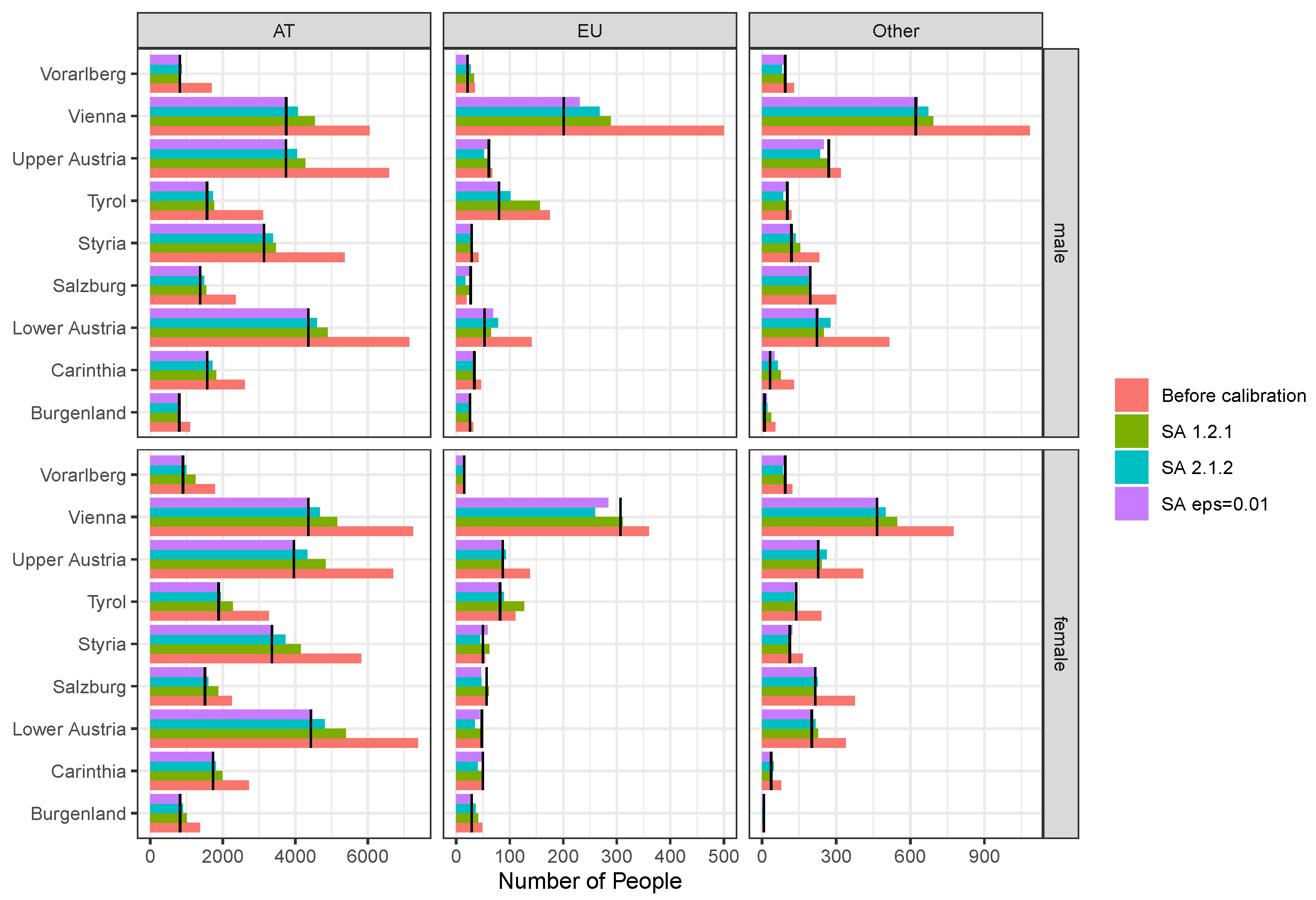
3.6. Application of the SA Algorithm

The SA algorithm including the improvements is fully implemented in the function calibPop() in the R package simPop. Some parameters have been added that reflect various hyperparameters described above (see Appendix B.4).

For demonstration purposes, we post-calibrate the synthetic population from the previous section and use the data set eusilcP as the target population. We choose the following two post-calibration scenarios to highlight the improvements to the algorithm:

• Post-calibrate the synthetic population on a single target margin using the number of individuals by region, gender and citizenship
• Post-calibrate the synthetic population on two target margins using the number of individuals by region, gender and citizenship and number of households by region and household size.

In both scenarios, a value of $ϵ=0.1$ was set as default. The R code to apply the post-calibration scenarios to the synthetic data can be found in the Appendix C under Appendices Appendix C.4 and Appendix C.5. We performed this calculation on a server running Ubuntu 18.04 Intel(R) Xeon(R) CPU E5-2690 v4 @ 2.60 GHz with 8 cores and 125 GB memory. With the improved version of SA using only the single target margin, the algorithm converges in a few seconds instead of almost 50 min when using the older version implemented in simPop 1.2.1. When running the improved version with $ϵ=0.01$, it converges in almost 10 s.

The results of the first scenario are shown in Figure 5, where the distribution of the variables used for post-calibration is displayed. The colors indicate the distribution before calibration, after calibration using the old implementation SA 1.2.1, the improved implementation SA 2.1.2 and the improved implementation using $ϵ=0.01$ SA eps = 0.01. The black lines represent the target distribution. Citizenship pb220a is shown in the horizontal panels and gender rb090 in the vertical panels. The distributions using the improved method seem to be more similar to the target margins, especially for large populations, e.g., the box on the left for people with the nationality “AT”. Table 2 shows the mean absolute error (MAE), the mean absolute percentage error (MAPE), as well as the average Aitchison distance (see [32,33]), compared to the target distribution. Using the improved implementation instead of the old, the MAE and MAPE are drastically reduced, especially for $ϵ=0.01$. For the average Aitchison distance, we observe similar values for the old and new improvements, but again a drastic improvement for $ϵ=0.01$.

Figure 5. Distribution of people after post-calibration by variables “db040”, citizenship (horizontal panels) and gender (vertical panels). Colored bars show the distribution after applying the old version of calibPop (SA 1.2.1), the improved version of calibPop (SA 2.1.2) and the improved version of calibPop with $ϵ=0.01$. The black lines represent the target distribution, the red bars the distribution before calibration.

Table 2. Mean absolute error, mean absolute percentage error and average Aitchison distance between target totals and population totals before and after calibration from the first scenario.

	MAE	MAPE	Avg. Aitchison
Before calibration	618.31	71.31	2.52
SA 1.2.1	158.47	22.13	1.68
SA 2.1.2	75.26	17.36	1.73
SA $ϵ=0.01$	8.02	7.41	1.27

Figure 6 shows the results of the second scenario using two target distributions—one for the number of individuals and one for the number of households As a comparison the distribution before calibration and the distribution using only one set of target margins are displayed. The upper part of the Figure 6 shows that the margins for the number of people are reproduced slightly worse when multiple margins are used. The distribution on the number of households is, however, represented better when also considered during calibration, as can be seen in the bottom part of Figure 6.

Figure 6. Distribution of people (left side) and households after post-calibration. The colors indicate using only one set of target margins (single margins) on people and target margins on people and households simultaneously (multiple margins). The black lines represent the target distribution, the red bars the distribution before calibration.

Table 3 shows the MAE, the MAPE and the average Aitchison distance compared to the target distribution for the second scenario. Using multiple margins yields slighter higher error measures for the person margins but much lower ones for the household margins. The household margins before the calibration yield a low average Aitchison distance because the relative distribution is already quite similar to the relative target distribution.

Table 3. Mean absolute error, mean absolute percentage error and average Aitchison distance between target totals and population totals before and after calibration from calibration from the first scenario.

		MAE	MAPE	Avg. Aitchison
	Before calibration	618.20	71.31	2.52
Person margins	Single margins	75.26	17.36	1.73
	Multiple margins	80.44	29.72	2.33
	Before calibration	280.22	40.03	0.31
Household margins	Single margins	113.19	16.83	1.24
	Multiple margins	54.72	9.75	0.48

4. Conclusions

Important improvements for the synthesis of complex data sets using the R package simPop were presented. Although the methods work to simulate synthetic data from simple structured data sets, they are also able to deal with more complex situations that are not addressed in the literature or other software. The methods can also be used for complex samples conducted with complex survey designs and calibrated samples that additionally contain information on multiple margins of different types of unit (e.g., persons and households). Thus, values on specified margins of the synthesized data correspond to the values of margins of the original data and/or the additional information on known population characteristics.

With the presented methods and tools, one can even create a whole population from a complex sample. This is especially important for micro-simulation and agent-based simulations. Hereby, in a first step, a population is generated with the help of our presented methods. For micro-simulation tasks, this population is then stochastically extrapolated up to a defined time horizon, taking into account various relevant scenarios, e.g., for policy measures, demographic development, migration, etc. The base population is then used as a proxy for the real and unknown population.

Another important feature not detailed in this paper is that the synthetic data set can be generated from multiple inputs. These inputs can be census or sample data.

The integration of XGBoost as a fully conditional simulation method into the R package simPop has been carried out in such a way that it fully matches the S4 class structure of the package to allow its application to data including the challenges mentioned. In addition, hyperparameter tuning is built-in—an important point in achieving better results than with fixed default settings. XGBoost has been shown to be a competitive method for synthesizing data. Realistic cluster structures and logical conditions are naturally considered by construction, and multiple relationships are considered by sequentially synthesizing variables.

After synthesizing the data, we developed a post-calibration to calibrate for multiple margins. It is now possible to calibrate against multiple margins even if they are defined for different types of units (e.g., persons and households) at the same time.

All of these improvements raise the simulation of synthetic data to a higher level and account for many practical and complex real-world problems.

Appendix B.1. Detailed Calibration Algorithm

Algorithm A1 presents the Simulated Annealing algorithm in more detail.

Algorithm A1 Detailed calibration algorithm

1:   Duplicate the synthetic population K times to include $N^{\prime }=N·K$ individuals, increasing the likelihood of finding a composition $({\delta }_1,\dots ,{\delta }_N)$. 2:   Set the initial conditions: Start temperature $T>0$ Cooling rate $r_T\in (0,1)$ Minimum temperature $T_{min}$ Maximum number of cooldowns $C>100$ Counter for number of cooldowns $N_C=1$ Initial number of selections/deselections $n=Obj·\frac{{\mathrm{med}}_{hsize}}{5}$ Reduction rate for number of swaps $r_n\in (0,1)$ Allowed relative error $ϵ>0$ Number of iterations until cooling c Counter for iterations until next cooldown $n_c=1$ 3:   Initialize a first selection $\Delta =({\delta }_1,\dots ,{\delta }_{N^{\prime }})$, calculate initial synthetic margins $\mathbf{m}$, and the value of the objective function: $$Obj=f(\mathbf{t},\widehat{\mathbf{t}})=\sum _{m=1}^M|t_m-{\widehat{t}}_m|$$ 4:   Randomly add and remove n persons, including all household members, from the selection $\Delta$ by setting ${\delta }_i=0$ or ${\delta }_i=1$ for each member of the drawn household, resulting in a new selection ${\Delta }_{new}$. 5:   Calculate the new value of the objective function $Ob{j}_{new}$ using ${\Delta }_{new}$. 6:   if $\frac{Ob{j}_{new}}{N}\le ϵ$ then 7:       Convergence reached, terminate the algorithm and return ${\Delta }_{new}$. 8:   end if 9:   if $Ob{j}_{new}<Obj$ then 10:     Update $\Delta \leftarrow {\Delta }_{new}$. 11: else 12:     Update current selection $\Delta$ with new selection ${\Delta }_{new}$ if $u<exp\left(-\frac{Ob{j}_{new}-Obj}{T}\right)$ where u is drawn from $U(0,1)$; otherwise, keep $\Delta$. 13: end if 14: Increment $n_c$; if $n_c>c$, start the next cooldown, otherwise, repeat from step 4: $n\leftarrow max(1,\lfloor n·r_n\rfloor )$ $T\leftarrow T·r_T$ $N_C\leftarrow N_C+1$ $n_c\leftarrow 1$ 15: if $N_C>C$ or $T<T_{min}$ then 16:     Terminate the algorithm and return current selection $\Delta$. 17: else 18:     Go to step 4. 19: end if

Appendix B.2. Initialise and Adjust Number of Swaps N

The convergence of the SA algorithm is greatly influenced by the initial number of swaps (n). Choosing a very high n can lead to frequent changes in $\Delta$ due to a high acceptance rate for a worse solution. In contrast, selecting a very low n can limit the potential to improve the objective function. Naturally, n should depend on the initial value of $f(\mathbf{t},\widehat{\mathbf{t}})$ and the size of the synthetic population. An initial choice of the swap rate n is as follows:

$$\begin{array}{c}\hfill n=min(\underset{m,r}{max}\left(\right|t_{m,r}-{\widehat{t}}_{m,r}\left|\right)·\frac{2}{3},0.05·\frac{N_P}{me{d}_{hsize}}).\end{array}$$

(A1)

The first part is related to the objective function, and the second to the size of the target population. This suggested starting value proved practical during the work in [29].

The swap rate n can also be controlled during the SA algorithm for faster convergence. When selecting or deselecting individuals, the whole household is chosen; thus, the number of individuals in the synthetic population can change, affecting the algorithm’s convergence. To address this, a scaling factor is introduced to maintain the total number of individuals or households at the same level as the target margins. Before the sampling step, the number of draws for the selection of persons and households to be included and excluded is adjusted by

$$n_{in}=max(\lceil n-gap\rceil ,1)$$

(A2)

$$n_{out}=max(\lceil n+gap\rceil ,1),$$

(A3)

where

$$gap=r_{re}·\frac{1}{{\displaystyle \sum _{r=1}^R}{M}_r}\left(\sum _{m=1}^M\sum _{r=1}^{R_m}{t}_{m,r}-{\widehat{t}}_{m,r}\right)$$

(A4)

$$\begin{array}{cc}\hfill r_{re}\in & (0,1).\hfill \end{array}$$

(A5)

For ${\displaystyle \sum _{r,t}}{t}_{m,r}-{\widehat{t}}_{m,r}>0$, the number of individuals or households selected is overall smaller than the target population margins. Multiplying with the factor $\frac{1}{{\displaystyle \sum _{r=1}^R}{M}_r}$ yields an estimate of the average number of individuals or households missing in each of the margin cells of the synthetic population. On the other hand ${\displaystyle \sum _{r,t}}{t}_{m,r}-{\widehat{t}}_{m,r}<0$ implies that too many individuals or households have been selected. The value $gap$ is, thus, an estimated difference to the desired total population in terms of individuals $N_P$ or households $N_H$. Considering Equations (A2) and (A3), it is clear to see that choosing $r_{re}=1$ would imply that $n_{in}$ and $n_{out}$ can overcompensate for this difference calculated in Equation (A4) and the solutions would likely begin to jump above and below the desired total ${\displaystyle \sum _{t=1}^{M_r}}{t}_{m,r}$. With a value of $r_{re}=0.5$, half of the estimated difference is addressed when adding and removing individuals from the current selection. Thus, the value of $r_{re}=0.5$ is recommended to stabilize the solutions.

Appendix B.3. Automatically Choosing T and Forcing Cooldowns

The starting temperature T can strongly influence the convergence of the SA. If T is chosen too high, the algorithm jumps aimlessly through the search space and, depending on the cooling rate $r_T$, it takes some time for the SA to narrow down to a solution. If T, on the other hand, is chosen too small, the SA may become stuck in a local optimum too early and have no possibility to improve further. The starting temperature $T_{adj}$ can optionally be adjusted automatically in the initialization phase of the SA by

$$T_{adj}=max(T,r_a\frac{1}{{\displaystyle \sum _{r=1}^R}{M}_r}\sum _{m=1}^M\sum _{r=1}^{R_m}{t}_{m,r}{ϵ}_m)$$

(A6)

$${ϵ}_m=\left\{\begin{array}{c}{ϵ}_H\mathrm{if}{\mathbf{t}}_{\mathbf{m}}\mathrm{corresponds}\mathrm{to}\mathrm{household}\mathrm{margins}\hfill \\ {ϵ}_P\mathrm{if}{\mathbf{t}}_{\mathbf{m}}\mathrm{corresponds}\mathrm{to}\mathrm{person}\mathrm{margins}\hfill \end{array}\right.$$

(A7)

$$\begin{array}{cc}\hfill m=& 1,\dots ,M,\hfill \end{array}$$

(A8)

where $r_a\in (0,1)$. Besides the individual adjustment of T, the SA algorithm can become stuck between cooldowns and further improvements of the current solution can only be achieved after successive cooldowns with decreasing T as well as n. Since c usually sets the number of iterations between cooldowns to several hundreds, we implemented a procedure that forces a cooldown if the value of the objective function has not changed since h iterations and the previous h values of the objective function, $Ob{j}_1,\dots ,Ob{j}_h$, satisfy

$$\begin{array}{c}\hfill \frac{{\sigma }_{Obj}}{\overline{Obj}}<r_h,\end{array}$$

(A9)

with ${\sigma }_{Obj}$ as the standard deviation and $\overline{Obj}$ as the arithmetic mean of $Ob{j}_1,\dots ,Ob{j}_h$. This addition has the sole purpose of decreasing the number of iterations if the solution starts to become stuck for a given n and T. For the work in [29], we chose $r_a=0.2$ and $r_h=0.05$.

Appendix B.4. Hyperparameters in Package simPop for Population Calibration

Table A3 shows the connection of parameters in the equations above to function arguments in the software implementation.

Table A3. Some of the new function arguments of function calibPop().

Function Argument	Parameter
choose.temp.factor	$r_a$
scale.redraw	$r_{re}$
observe.times	h
observe.break	$r_h$
hhTables, persTables	${\mathbf{t}}_1,\dots ,{\mathbf{t}}_M$

Table A3. Some of the new function arguments of function calibPop().

Function Argument	Parameter
choose.temp.factor	$r_a$
scale.redraw	$r_{re}$
observe.times	h
observe.break	$r_h$
hhTables, persTables	${\mathbf{t}}_1,\dots ,{\mathbf{t}}_M$

We refer to other newly added parameters, such as splitUpper, redist.var and redist.var.factor, to the help page ?calibPop. They can be useful for calibrating synthetic data with a high geographic resolution, such as local administrative units level 2 (LAU2) or more granular.

Appendix C.1. Simulation of Synthetic Data with XGBoost

The following code snipped shows how to simulate a cluster structure in software R. To generate the household structure, first, the data input is specified naming the data set, the (optional) cluster structure, the (optional) stratification variable(s) (in each strata, the simulation is taken independently), and the (optional) vector of sampling weights. Secondly, the function simStructure is used, with the basic household variables specified in the function argument basicHHvars. Note that there are different methods available, such as “direct” with estimation of the population totals for each combination of stratum and household size using the Horvitz–Thompson estimator, “multinom” with the estimation of the conditional probabilities within the strata using a multinomial log-linear model and random draws from the resulting distributions, or “distribution” with random draws from the observed conditional distributions within the strata.

R> library(simPop)

R> ## load the demo data set

R> data(eusilcS)

R>

R> ## create the structure

R> inp <- specifyInput(data = eusilcS,

R>                  hhid = "db030",   # variable with cluster information

R>                  strata = "db040", # optional stratification

R>                  weight = "db090") # variable with sampling weights

R>

R>

R> simPop <- simStructure(data = inp,    # data structure

R>                        method = "direct",

R>                        basicHHvars = c("age", "rb090"))

In doing so, simStructure requires all information about the structure of a data set. For surveys with complex sampling designs, more information has to be provided (e.g., function argument weight) than for the simulation of survey samples obtained with simple random sampling or by simulating census data. In our case, the data set is collected on the basis of a complex sample design, and in addition, there is a household structure, e.g., all persons within a household are surveyed (function argument hhid). To reflect heterogeneity in the population, samples are often drawn within strata, e.g., regions (functional argument strata). Note that specifyInput generates a S4-class object [36] including all necessary information.

R> class(simPop)

[1] "simPopObj"

attr(,"package")

The implemented print method already shows some basic information.

R> simPop

--------------

synthetic population  of size

 81838 x 7

build from a sample of size

 11725 x 20

--------------

variables in the population:

db030,hhsize,db040,age,rb090,pid,weight

Appendix C.2. Synthesizing Additional Variables

In the example below, two new variables, "pl030" (person’s economic status) and "pb220a" (citizenship)), are simulated for the population. All function arguments and parameters for the xgboost algorithm can be passed through model_params. The complete list of the hyperparameters is listed in [37].

R> model_params <- list(max.depth = 10, # maximum depth of a tree

R>                     eta = 0.5,      # learning rate

R>                     nrounds = 5,    # max number of boosting iterations

R>                     objective = "multi:softprob") # softmax objective

R>

R> simPop <- simCategorical(simPop,

R>                          additional = c("pl030", "pb220a"),

R>                          method = "xgboost",

R>                          model_params = model_params)

The print method shows the successful simulation of these two new variables.

R> simPop

--------------

synthetic population  of size

 81838 x 9

build from a sample of size

11725 x 20

--------------

variables in the population:

db030,hhsize,db040,age,rb090,pid,weight,pl030,pb220a

The population now consists of the basic variables, the structure variables and the newly generated categorical variables ("pl030" (person’s economic status) and "pb220a" (citizenship)). Table A4 displays a snippet of the initial five observations from the already simulated data.

Table A4. An excerpt of the synthetic population generated by the proposed XGBoost approach.

	db030	hhsize	db040	Age	rb090	Pid	Weight	pl030	pb220a
1	4570	1	Lower Austria	68	male	4570.1	1.00	5	AT
2	1735	1	Carinthia	65	male	1735.1	1.00	5	AT
3	655	2	Burgenland	55	female	655.1	1.00	5	AT
4	836	3	Burgenland	64	female	836.1	1.00	7	AT
5	2984	4	Carinthia	13	female	2984.4	1.00	4	AT

Table A4. An excerpt of the synthetic population generated by the proposed XGBoost approach.

	db030	hhsize	db040	Age	rb090	Pid	Weight	pl030	pb220a
1	4570	1	Lower Austria	68	male	4570.1	1.00	5	AT
2	1735	1	Carinthia	65	male	1735.1	1.00	5	AT
3	655	2	Burgenland	55	female	655.1	1.00	5	AT
4	836	3	Burgenland	64	female	836.1	1.00	7	AT
5	2984	4	Carinthia	13	female	2984.4	1.00	4	AT

Appendix C.3. Hyperparameter Tuning for XGBoost

R> grid <- expand.grid(nrounds = c(5, 10),

R>                     max_depth = 10,

R>                     eta = c(0.2, 0.3, 0.5),

R>                     eval_metric = "mlogloss",

R>                     stringsAsFactors = F)

R> additionals <- c("pl030", "pb220a")

R>

R> # Remove variables and regenerate with crossValidation

R> simPop@pop@data[, (additionals) := NULL]

R>

R> simPop <- crossValidation(simPop,

R>                           additionals = additionals,

R>                           fold = 3, #

R>                           hyper_param_grid = grid)

R>

R> simPop

--------------

synthetic population  of size

 81838 x 9

build from a sample of size

11725 x 20

--------------

variables in the population:

db030,hhsize,db040,age,rb090,pid,weight,pl030,pb220a

Appendix C.4. Post-Calibration First Scenario

R> data(eusilcP) # use to derive target margins

R>

R> # build target margins

R> margins <- xtabs( ^~ region + gender + citizenship,

R>                  data = eusilcP)

R> margins <- as.data.frame(margins)

R> # rename to match column names in synthetic data

R> colnames(margins) <- c("db040", "rb090", "pb220a", "freq")

R>

R> # add target margins to simPop-object

R> simPop <- addKnownMargins(simPop, margins)

R> # apply simulated annealing for each "db040"

R> simPop_adj <- calibPop(simPop,

R>                        split = "db040",

R>                        epsP.factor = 0.1,

R>                        choose.temp = TRUE,

R>                        choose.temp.factor = 0.2,

R>                        nr_cpus = 1,

R>                        verbose = FALSE)

Appendix C.5. Post-Calibration Second Scenario

R> # target margins for persons

R> persTables <- xtabs(^~ region + gender + citizenship,

R>                     data = eusilcP)

R> persTables <- as.data.frame(persTables)

R> colnames(persTables) <- c("db040", "rb090", "pb220a", "Freq")

R>

R> # target margins for households

R> filter_hid <- !duplicated(eusilcP$hid)

R> # re-code household size

R> eusilcP$hsize4 <- pmin(4, as.numeric(eusilcP$hsize))

R> simPop@pop@data$hhsize4 <- pmin(4, as.numeric(simPop@pop@data$hhsize))

R>

R> hhTables <- xtabs(^~ region + hsize4,

R>                   data = eusilcP[filter_hid, ])

R> hhTables <- as.data.frame(hhTables)

R> colnames(hhTables) <- c("db040", "hhsize4", "Freq")

R>

R> # run simulated annealing

R> simPop_adj_2tables <- calibPop(simPop, split = "db040",

R>                                temp=1, epsP.factor = 0.1,

R>                                epsH.factor = 0.1,

R>                                persTables = persTables,

R>                                hhTables = hhTables,

R>                                nr_cpus = 1, verbose = TRUE)

References

1. United Nations Economic Commission for Europe. Synthetic Data for Official Statistics: A Starter Guide; Technical Report, Report No. ECE/CES/STAT/2022/6; United Nations: Rome, Italy, 2022. [Google Scholar]
2. Dwork, C. Differential Privacy. In International Colloquium on Automata, Languages, and Programming; Springer: Berlin/Heidelberg, Germany, 2006; pp. 1–12. [Google Scholar] [CrossRef]
3. Fischetti, M.; Salazar-González, J. Complementary Cell Suppression for Statistical Disclosure Control in Tabular Data with Linear Constraints. J. Am. Stat. Assoc. 2000, 95, 916–928. [Google Scholar] [CrossRef]
4. Enderle, T.; Giessing, S.; Tent, R. Calculation of Risk Probabilities for the Cell Key Method. In Privacy in Statistical Databases: UNESCO Chair in Data Privacy, Proceedings of the International Conference PSD 2020, Tarragona, Spain, 23–25 September 2020; Springer: Berlin/Heidelberg, Germany, 2020; pp. 151–165. [Google Scholar] [CrossRef]
5. Novák, J.; Sixta, J. Visualization of Record Swapping. Austrian J. Stat. 2024, 53, 1–16. [Google Scholar] [CrossRef]
6. Yin, X.; Zhu, Y.; Hu, J. A Comprehensive Survey of Privacy-Preserving Federated Learning: A Taxonomy, Review, and Future Directions. ACM Comput. Surv. 2021, 54, 1–36. [Google Scholar] [CrossRef]
7. Templ, M.; Alfons, A. Disclosure Risk of Synthetic Population Data with Application in the Case of EU-SILC. In Privacy in Statistical Databases; Lecture Notes in Computer Science; Springer: Berlin/Heidelberg, Germany, 2010; pp. 174–186. [Google Scholar] [CrossRef]
8. Templ, M. Providing Data with High Utility and No Disclosure Risk for the Public and Researchers: An Evaluation by Advanced Statistical Disclosure Risk Methods. Austrian J. Stat. 2014, 43, 247–254. [Google Scholar] [CrossRef]
9. McClure, D.; Reiter, J. Assessing Disclosure Risks for Synthetic Data with Arbitrary Intruder Knowledge. Stat. J. IAOS 2016, 32, 109–126. [Google Scholar] [CrossRef]
10. Alfons, A.; Kraft, S.; Templ, M.; Filzmoser, P. Simulation of Close-to-Reality Population Data for Household Surveys with Application to EU-SILC. Stat. Methods Appl. 2011, 20, 383–407. [Google Scholar] [CrossRef]
11. Templ, M.; Filzmoser, P. Simulation and Quality of a Synthetic Close-to-Reality Employer–Employee Population. J. Appl. Stat. 2014, 41, 1053–1072. [Google Scholar] [CrossRef]
12. Münnich, R.; Schürle, J. On the Simulation of Complex Universes in the Case of Applying the German Microcensus; DACSEIS Research Paper Series No. 4; University of Tübingen: Tubingen, Germany, 2003. [Google Scholar]
13. Nowok, B.; Raab, G.; Dibben, C. synthpop: Bespoke Creation of Synthetic Data in R. J. Stat. Softw. 2016, 74, 1–26. [Google Scholar] [CrossRef]
14. Templ, M.; Meindl, B.; Kowarik, A.; Dupriez, O. Simulation of Synthetic Complex Data: The R Package simPop. J. Stat. Softw. 2017, 79, 1–38. [Google Scholar] [CrossRef]
15. Mendelevitch, O.; Lesh, M. Beyond Differential Privacy: Synthetic Micro-Data Generation with Deep Generative Neural Networks. In Security and Privacy from a Legal, Ethical, and Technical Perspective; IntechOpen: London, UK, 2020; pp. 1–14. [Google Scholar] [CrossRef]
16. Solatorio, A.V.; Dupriez, O. REaLTabFormer: Generating Realistic Relational and Tabular Data using Transformers. arXiv 2023, arXiv:2302.02041. [Google Scholar] [CrossRef]
17. Särndal, E. The Calibration Approach in Survey Theory and Practice. Surv. Methodol. 2007, 33, 99–119. [Google Scholar]
18. Horvitz, D.G.; Thompson, D.J. A Generalization of Sampling Without Replacement from a Finite Universe. J. Am. Stat. Assoc. 1952, 47, 663–685. [Google Scholar] [CrossRef]
19. Walker, A.J. An Efficient Method for Generating Discrete Random Variables with General Distributions. ACM Trans. Math. Softw. (TOMS) 1977, 3, 253–256. [Google Scholar] [CrossRef]
20. Chen, T.; Guestrin, C. XGBoost: A Scalable Tree Boosting System. In Proceedings of the 22nd ACM SIGKDD International Conference on Knowledge Discovery and Data Mining, KDD ‘16, New York, NY, USA, 13–17 August 2016; pp. 785–794. [Google Scholar] [CrossRef]
21. Johnson, R.; Zhang, T. Learning Nonlinear Functions Using Regularized Greedy Forest. IEEE Trans. Pattern Anal. Mach. Intell. 2013, 36, 942–954. [Google Scholar] [CrossRef] [PubMed]
22. Brandt, S. Statistical and Computational Methods in Data Analysis. Am. J. Phys. 1971, 39, 1109–1110. [Google Scholar] [CrossRef]
23. Vorhies, W. Want to Win Competitions? Pay Attention to Your Ensembles. 2016. Available online: https://www.datasciencecentral.com/profiles/blogs/want-to-win-at-kaggle-pay-attention-to-your-ensembles (accessed on 25 February 2021).
24. Huang, Z.; Williamson, P. A Comparison of Synthetic Reconstruction and Combinatorial Optimization Approaches to the Creation of Small-Area Micro Data; Working Paper 2001/02; Department of Geography, University of Liverpool: Liverpool, UK, 2001. [Google Scholar]
25. Voas, D.; Williamson, P. An Evaluation of the Combinatorial Optimisation Approach to the Creation of Synthetic Microdata. Int. J. Popul. Geogr. 2000, 6, 349–366. [Google Scholar] [PubMed]
26. Kirkpatrick, S.; Gelatt, C.; Vecchi, M. Optimization by Simulated Annealing. Science 1983, 220, 671–680. [Google Scholar] [CrossRef] [PubMed]
27. Cerný, V. Thermodynamical Approach to the Traveling Salesman Problem: An Efficient Simulation Algorithm. J. Optim. Theory Appl. 1985, 45, 41–51. [Google Scholar] [CrossRef]
28. Harland, K.; Heppenstall, A.; Smith, D.; Birkin, M. Creating Realistic Synthetic Populations at Varying Spatial Scales: A Comparative Critique of Population Synthesis Techniques. J. Artif. Soc. Soc. Simul. 2012, 15, 1. [Google Scholar] [CrossRef]
29. Rubinyi, S.; Verschuur, J.; Goldblatt, R.; Gussenbauer, J.; Kowarik, A.; Mannix, J.; Bottoms, B.; Hall, J. High-Resolution Synthetic Population Mapping for Quantifying Disparities in Disaster Impacts: An Application in the Bangladesh Coastal Zone. Front. Environ. Sci. 2022, 10, 1033579. [Google Scholar] [CrossRef]
30. Minnesota Population Center. Integrated Public Use Microdata Series, International: Version 7.3 [Dataset]; IPUMS: Minneapolis, MN, USA, 2020. [Google Scholar] [CrossRef]
31. Müller, K. wrswoR: Weighted Random Sampling without Replacement; R package Version 1.1.1. 2020. Available online: https://CRAN.R-project.org/package=wrswoR (accessed on 1 May 2024).
32. Fačevicová, K.; Hron, K.; Todorov, V.; Templ, M. Compositional Tables Analysis in Coordinates. Scand. J. Stat. 2016, 43, 962–977. [Google Scholar] [CrossRef]
33. Fačevicová, K.; Hron, K.; Todorov, V.; Templ, M. General approach to coordinate representation of compositional tables. Scand. J. Stat. 2018, 45, 879–899. [Google Scholar] [CrossRef]
34. Alfons, A.; Templ, M. Estimation of Social Exclusion Indicators from Complex Surveys: The R Package laeken. J. Stat. Softw. 2013, 54, 1–25. [Google Scholar] [CrossRef]
35. Templ, M. Imputation and Visualization of Missing Values; Springer International Publishing: Cham, Switzerland, 2023; p. 561, in print. [Google Scholar]
36. Chambers, J. Extending R; Chapman & Hall/CRC the R Series; CRC Press, Taylor & Francis Group: Boca Raton, FL, USA, 2016. [Google Scholar]
37. XGBoost Developers. XGBoost Parameters. 2020. Available online: https://xgboost.readthedocs.io/en/latest/parameter.html (accessed on 15 December 2020).