Research on Distributed Fault Diagnosis Model of Elevator Based on PCA-LSTM

Abstract

A Distributed Elevator Fault Diagnosis System (DEFDS) is developed to tackle frequent malfunctions stemming from the widespread distribution and aging of elevator systems. Due to the complexity of elevator fault data and the subtlety of fault characteristics, traditional methods such as visual inspections and basic operational tests fall short in detecting early signs of mechanical wear and electrical issues. These conventional techniques often fail to recognize subtle fault characteristics, necessitating more advanced diagnostic tools. In response, this paper introduces a Principal Component Analysis–Long Short-Term Memory (PCA-LSTM) method for fault diagnosis. The distributed system decentralizes the fault diagnosis process to individual elevator units, utilizing PCA’s feature selection capabilities in high-dimensional spaces to extract and reduce the dimensionality of fault features. Subsequently, the LSTM model is employed for fault prediction. Elevator models within the system exchange data to refine and optimize a global prediction model. The efficacy of this approach is substantiated through empirical validation with actual data, achieving an accuracy rate of 90% and thereby confirming the method’s effectiveness in facilitating distributed elevator fault diagnosis.

1. Introduction

With the rapid urbanization and proliferation of high-rise buildings, the number of elevators in use has significantly increased. Consequently, elevators frequently face issues such as entrapment, overshooting the top floor, or experiencing slippage. These operational challenges not only cause considerable inconvenience but also pose potential hazards. Thus, there is a critical need for the development and research of advanced elevator failure prediction systems. By predicting failures in advance, it is possible to prevent accidents and minimize operational downtime, thereby enhancing the safety and reliability of elevator operations. The data from elevator operations, which are spatially distributed, are typically centralized in data centers. This centralization of data for fault analysis often overloads the central processors, resulting in slower detection times. Therefore, developing a distributed elevator fault prediction system capable of diagnosing faults across multiple elevators holds significant importance.

A substantial body of research has been conducted both domestically and internationally on the prediction of elevator faults, predominantly utilizing mathematical or physical models of elevator equipment. Lu et al. [1] employed Convolutional Neural Networks (CNNs) to automate fault diagnosis using data gathered from elevator vibration sensors, significantly reducing the time and effort required for fault information collection. Traditional expert systems, when faced with elevator faults, often exhibit low diagnostic accuracy due to challenges in data acquisition and limited learning capabilities. To address this, Liang et al. [2] developed an elevator door system fault diagnosis model based on the XGBoost algorithm, which effectively identifies the presence and type of faults in the elevator door system from extensive diagnostic data. The fault diagnosis of critical mechanical components is essential for ensuring passenger safety and comfort. Zheng et al. [3] tackled the issues of noise and indirect signal acquisition by analyzing micro-impact signals resulting from mechanical damage, using real-time data from elevator operations to enable intelligent fault diagnosis. Zhang et al. [4] devised a deep convolutional forest algorithm to model elevator door fault diagnosis based on comprehensive elevator operation and maintenance data, employing CNNs for feature extraction and the deep forest algorithm as a classifier to pinpoint faults. Addressing the sample imbalance between elevator factory samples and fault samples, Qiu et al. [5] proposed an improved fault diagnosis method for imbalanced samples using the Aquila optimizer-enhanced Extreme Gradient Boosting Trees (XGBoost). Chen et al. [6] considered the time and frequency domain characteristics of elevator car vibration faults and developed a simple mathematical model combining a radial basis function (RBF) neural network to predict elevator car vibration fault diagnosis outcomes. Liang et al. [7] utilized fault tree analysis to pinpoint and rectify faults. Wu et al. [8] applied a combination of the polar band algorithm (PBO) and CNN to detect faults in elevator bearings based on vibration signals during operation. Li et al. [9] introduced a multichannel, one-dimensional convolutional neural network for diagnosing abnormal elevator vibration faults, effectively leveraging elevator vibration data. Considering the sensitivity of traction wheel-bearing fault diagnosis to variable speed conditions and environmental noise, Yi et al. [10] introduced an angular-domain resampling method for estimating traction wheel rotational speed and a traction wheel-bearing fault diagnosis method optimized using the Sparrow Search Algorithm (SSA). Jin et al. [11] proposed an elevator fault identification and judgment method based on kernel entropy component analysis (KECA), performing dimensionality reduction and clustering analysis on various types of elevator fault data. Finally, Liu Ying et al. [12] developed a neural network-based elevator fault diagnosis system optimized using a genetic algorithm, aiming to overcome the challenges associated with obtaining mathematical models of elevator systems and diagnosing operational dynamics.

Bai et al. [13] employed mathematical computing mechanisms to analyze the characteristics of a research object and successfully developed an elevator fault prediction model utilizing the optimized PSO-BP (Particle Swarm Optimization–Back Propagation) algorithm. Additionally, Chen et al. [14] provided a comprehensive overview of a variety of AI algorithms for elevator fault diagnosis at both theoretical and application levels. These algorithms include Back Propagation (BP) neural networks, Radial Basis Function (RBF) networks, K-means clustering, and Support Vector Machines (SVMs). They also conducted an extensive literature review on the applications of these algorithms in elevator fault diagnosis, drawing insights from their extensive body of work.

Most existing research on elevator fault diagnosis has primarily utilized machine learning techniques to identify faults in individual elevators. However, a significant portion of the literature has also explored the use of distributed methods, which are applied not only for fault detection but also for the precise localization of faults across elevator systems. This broader approach addresses both system-wide issues and specific component malfunctions, thereby offering a comprehensive perspective that is crucial for advancing the field. Numerous studies have focused on fault diagnosis using distributed algorithms. For instance, Wang et al. successfully implemented a distributed deep learning model that utilizes geolocation by processing features as data through the hidden parameters of deep learning [15]. Jan et al. designed a distributed sensor-fault detection and diagnosis system utilizing a machine learning approach in which the fault detection is executed directly within the sensor to enable immediate output generation after data collection [16]. Conversely, Ali Murad and other researchers have employed various machine learning methods to classify and identify faults in cascaded H-bridge multilevel inverters (CHMLI) across different environments, demonstrating the widespread applicability of these algorithms for fault detection and localization in the distributed genset CHMLI [17].

For the collected elevator operation signals, affected due to Gaussian noise, issues such as variable and high dimensionality, as well as numerous types of faults and uneven sample distribution, arise. In this study, we utilized PCA to reduce the dimensionality of data, building on the advantages highlighted in previous literature. Subsequently, based on the characteristics of the elevator samples, we designed an LSTM model to determine the causes of failures and predict failure parameters. This model analyzes failure data to proactively provide failure warnings and significantly enhance elevator safety. A large body of related literature confirms that distributed fault diagnosis techniques can effectively manage the problem of overloaded central processors in complex systems. Common and frequently occurring faults are addressed independently by installing local intelligence on each elevator. Simultaneously, neighboring elevators in a distributed system can leverage their resources for model integration. To facilitate the exchange of model parameters, it is necessary to install management intelligence on multiple elevators in order to enable fault diagnosis across multiple units.

The main contributions of this paper are as follows: (1) the development of a fault diagnosis system based on the PCA-LSTM model for a single elevator and (2) the implementation of distributed communication among multiple elevators within the same network, in which the elevators act as nodes to exchange models with each other in order to optimize the fault diagnosis model.

The rest of the paper is structured as follows: Section 2 describes the fault diagnosis model for a single elevator. Section 3 details the implementation of the distributed fault diagnosis prediction system. Section 4 is the experimental section. Section 5 provides a summary.

2. PCA-LSTM Based Fault Prediction Model

2.1. Introduction to Principal Component Analysis (PCA)

Principal Component Analysis (PCA) is a widely used unsupervised learning technique that transforms observed data containing linearly correlated variables into a smaller number of linearly independent variables, known as principal components. Since the number of principal components is typically fewer than the original variables, PCA serves as an effective dimensionality reduction method. It not only reveals the fundamental structure of the data, that is, the intrinsic relationships among variables but is also commonly used as a preprocessing step for other machine learning methods. In the context of elevator operations, each fault data point may be caused by multiple fault characteristics. However, there may be redundancy among some of these characteristics, and using all these features directly for fault diagnosis could increase the training time of machine learning models and affect their accuracy. Therefore, dimensionality reduction to retain the most critical fault characteristics is particularly important and does not compromise the overall diagnostic effectiveness. In this study, we applied PCA to elevator fault data for dimensionality reduction, and we input the processed data into an LSTM model for further analysis. In selecting the principal components within PCA, we first assessed the characteristics of the dataset, including the volume of data, the feature distribution, and the relationship between features and common types of faults. Depending on the specifics of the dataset, we chose those principal components that contributed the most to the variance, which are typically able to capture the key variations in the fault data. Additionally, we considered the interpretability of the data, choosing principal components that can intuitively explain the fault phenomena, thus facilitating an understanding of the model’s output and effective fault diagnosis. In this way, PCA not only helps us simplify the data structure but also ensures that critical information necessary for fault diagnosis is not lost during the dimensionality reduction process. When applying PCA to elevator fault diagnosis, we usually follow the steps applied in the current research.

In this study, we first applied Principal Component Analysis (PCA) to the multidimensional sensor data collected during elevator operations, such as speed, vibration, and temperature data. The elevator fault data are characterized by high dimensionality, containing a substantial amount of redundancy and noise. By implementing PCA, we were able to effectively identify and retain the most influential features for fault type determination while eliminating irrelevant noise. Operationally, we chose principal components that accounted for over 85% of the variance in the original dataset. This threshold was determined based on an analysis of the characteristics of elevator fault data, with the aim of preserving the maximum amount of information critical to diagnosing elevator faults. For instance, if preliminary analysis indicated that vibration and temperature indicators were particularly important for predicting certain types of faults, the principal components associated with these indicators would be prioritized during the PCA process.

The initial step in preprocessing the elevator dataset, which consists of n samples each with m features forming an n × m dimensional matrix, X_nm, is to organize the data points to facilitate further analysis.

$$\left[\begin{array}{cccc}{x}_{11}& x_{12}& \cdots & x_{1m}\\ x_{21}& x_{22}& \cdots & x_{2m}\\ ⋮& ⋮& \ddots & ⋮\\ x_{n1}& x_{n2}& \cdots & x_{nm}\end{array}\right]$$

(1)

Step 1. Data normalization.

Normalize the data $X_{nm}$ for each feature normalized to a mean of 0 and a root mean square of 1.

$$x_{i,j}^{*}=\left(x_{i,j}-\overline{x_i}\right)/\sqrt{S_i}$$

(2)

Among them is the following:

$$\overline{x_i}=\frac{1}{n}{\sum }_{j=1}^n{x}_{ji},i=1,2,\dots ,n$$

(3)

$$S_i=\frac{1}{n-1{\sum }_{j=1}^n{\left(x_{ji}-\overline{x_i}\right)}^2},i=1,2,\dots ,n$$

(4)

Step 2. Find the covariance matrix, R.

The covariance matrix is given by $R=\frac{1}{n-1}{X}^{T}X$.

The computed covariance matrix is an eigen m × m dimensional matrix.

Step 3. Find eigenvalues and eigenvectors.

Find the eigenvalues and eigenvectors of the covariance matrix R, and arrange the eigenvalues from smallest to largest.

$${\lambda }_1\ge {\lambda }_2\ge {\lambda }_3\dots \ge {\lambda }_m$$

(5)

The eigenvectors are obtained by rearranging them according to their eigenvalues: $P_{mm}=\left[p_1,p_2,\dots ,p_m\right]$.

Step 4. Select appropriate k features for PCA down-scaling.

In this study, the top k features with cumulative feature values greater than 85% were selected for PCA dimensionality reduction.

$${\sum }_{i=1}^k{\lambda }_i/{\sum }_{i=1}^m{\lambda }_i\ge 0.85$$

(6)

Figure 1 illustrates the proportion of variance explained by each principal component within the dataset derived from elevator experiments, demonstrating the rationale for adopting 85% as the threshold. The y-axis represents the percentage of the total variance explained by all principal components, while the x-axis indicates the sequentially numbered principal components. The stepwise blue line indicates the cumulative variance explained by the principal components as we progress from left to right (from the first to the last principal component). Each upward step signifies an increment in the total variance explained upon the inclusion of that component. The dashed red line across the graph marks the threshold of 85% cumulative explained variance. The point where this line intersects with the step curve (cumulative explained variance) signifies the minimum number of principal components necessary to explain at least 85% of the total variance. In this particular example, the intersection occurs at the 15th principal component (PC15), as annotated on the plot. This indicates that the first 15 principal components together explain 85% of the total variance. Hence, retaining these 15 components would capture the majority of the information present in the dataset while excluding the remaining components that contribute less significantly to the variance, which likely represent noise or less informative aspects of the data. Therefore, selecting components that encompass 85% of the variance is a justified approach, as it ensures the comprehensive capturing of the data structure while also reducing complexity and the potential for overfitting. It strikes a balance between information retention and computational efficiency.

Let the first k eigenvalues from largest to smallest form a diagonal matrix and the k corresponding eigenvectors form a descending matrix. That is,

$$S_{kk}=diag\left({\lambda }_1,{\lambda }_2,\dots ,{\lambda }_k\right)$$

(7)

$$P_{mk}=\left[p_1,p_2,\dots ,p_k\right]$$

(8)

After the PCA dimensionality reduction, the number of elevator samples is still n, but the number of features becomes k, and the dimensionality reduction formula is

$${\tilde{X}}_{nk}=X_{nm}*P_{mk}$$

(9)

The reconstruction of X to obtain the $X^{\prime }$ of the matrix is given by the formula

$$X^{\prime }={\tilde{X}}_{nk}{P}_{mk}^T=X_{nm}\ast P_{mk}{P}_{mk}^T$$

(10)

Based on the above calculations, it is known that PCA not only reduces the number of subsequent calculations but also improves overall performance.

2.2. Long Short-Term Memory’s Introduction to Neural Networks (LSTM)

The Long Short-Term Memory Neural Network (LSTM) represents an advancement over the traditional Recurrent Neural Network (RNN) architecture, and it is specifically engineered to overcome the challenges of vanishing and exploding gradients that are commonly encountered when training RNNs with long sequence data. By incorporating memory cells that enable the retention and manipulation of information over extended sequences, LSTMs provide a more robust framework for capturing temporal dependencies without losing significant gradients throughout the learning process. A key enhancement in LSTM is the addition of three control gates based on the RNN architecture: the input gate, output gate, and forget gate. The overall structure of the LSTM is illustrated in Figure 2.

Regarding the configuration of the Long Short-Term Memory (LSTM) network, we designed the network architecture to align with the time series characteristics of the elevator fault data. Given the time dependency and periodic variations in the elevator data, we opted for a two-layer LSTM structure to enhance the model’s learning capability. Each layer contains 100 neurons, a number that was determined through testing various model capacities and that demonstrated optimal performance in fault diagnosis. Furthermore, to address potential nonlinear relationships and complex temporal dynamics, we conducted a detailed hyperparameter tuning of the LSTM model. This included selecting the learning rate (initially set to 0.001) and implementing a gradual decay strategy to optimize the training process. This choice of network parameters ensures the model’s ability to capture complex patterns within the elevator fault data while avoiding overfitting and ensuring the generalizability of the model.

The retention of the state from the previous moment to the current cell state is controlled via the forget gate. The forget gate filters the memory content and decides whether the stored data should be retained or discarded. Its computation is as follows:

$$f_t=\sigma \left(W_{xf}{x}_t+W_{hf}{h}_{t-1}+b_f\right)$$

(11)

In the equation, $f_t$ is the output of the forget gate, $\sigma$ is the activation function, which is chosen as the Sigmoid function, which outputs a range between 0 and 1, used to represent the degree of openness of the gate. $W_{xf}$ is the weight matrix between the current input and the forget gate, $x_t$ is the current input state, $W_{hf}$ is the weight matrix between the historical output and the forget gate, $h_{t-1}$ is the output state of the previous moment, and $b_f$ is the bias term for the forget gate.

The input gate is used to update the cell state, determining whether the cell can remember new information. The state of the previous moment and the current input information are fed into the activation function, yielding an output value between 0 and 1. This output decides the update of information. A value of 0 indicates unimportance, while 1 indicates importance. The state of the previous moment and the current input information from the previous step are also processed using the tanh function. The information is compressed between −1 and 1, yielding the candidate cell state. The output of the input gate is as follows:

$$i_t=\sigma \left(W_{xi}{x}_t+W_{hi}{h}_{t-1}+b_i\right)$$

(12)

In the equation, $i_t$ is the output of the input gate, $W_{xi}$ is the weight matrix between the input and the input gate, $W_{hi}$ is the weight matrix between the historical output and the input gate, and $b_i$ is the bias term for the input gate.

The candidate cell status is represented as follows:

$${\tilde{C}}_t=\mathit{tanh}\left(W_{xc}{x}_t+W_{hc}{h}_{t-1}+b_c\right)$$

(13)

In the equation, ${\tilde{C}}_t$ represents the candidate cell state, $W_{xc}$ is the weight matrix between the input and the cell state, $W_{hc}$ is the weight matrix between the historical output and the cell state, and $b_c$ is the bias term for the cell state. The tanh function is used to scale the values.

After obtaining the outputs of the forget gate and the input gate, the current cell state, $C_t$, is composed of two parts. One part is the information retention determined by multiplying the output of the forget gate with the cell state of the previous moment. The other part is the information added by multiplying the output of the input gate with the current candidate state. The cell state is represented as follows:

$$C_t=f_t{C}_{t-1}+i_t{\tilde{C}}_t$$

(14)

The output gate controls the final output of the cell state. The output of the output gate is multiplied by the current cell state information and then passed through the tanh function to obtain the cell output. The output of the output gate is represented as follows:

$$o_t=\sigma \left(W_{xo}{x}_t+W_{ho}{h}_{t-1}+b_o\right)$$

(15)

$$h_t=o_t\tan \mathrm{h}\left(C_t\right)$$

(16)

where $o_t$ is the output of the output gate, $W_{xo}$ is the weight matrix between the input and the output gate, $W_{ho}$ is the weight matrix between the historical output and the output gate, $b_o$ is the bias term for the output gate, $h_t$ is the cell output, and $C_t$ is the current cell state.

2.3. PCA-LSTM Fault Diagnosis Modeling

This paper proposes a fault diagnosis model that integrates Principal Component Analysis (PCA) and Long Short-Term Memory (LSTM) neural networks. The input signal consists of various operating data from the elevator collected under different conditions, and the output is the predicted fault type. To ensure accurate fault diagnosis, it is necessary to screen the elevator sampling data, which are then divided into a training set and a test set, as depicted in Figure 3. The specific steps are as follows.

Step 1: We began by categorizing the initial sample set based on elevator fault types, such as mechanical, electrical, and operational faults. Each category was then subjected to a linear transformation using PCA. The transformed cumulative contribution ratio for each fault category was used to select the most informative principal components, capturing the unique variance within each fault type. This approach enabled us to reduce the sample set size without losing the distinctive fault signatures associated with each category, yielding a new, condensed sample set that encapsulated diverse fault characteristics for enhanced diagnostic analysis.

Step 2: The new sample set data signals were transformed into a two-dimensional feature map. The samples were randomly selected proportionally and divided into two parts: the training set and the test set.

Step 3: The LSTM neural network was initialized, and the training set was input to train the LSTM network model.

Step 4: The test set was input into the trained network to classify the elevator fault types, and the diagnostic results were output.

3. Distributed Elevator Fault Diagnosis System

3.1. Overview of Diagnostic Methods

Elevator fault diagnosis represents an organic integration of sensor technology, embedded systems, network transmission, computer control, intelligent diagnostics, databases, and other cutting-edge technologies. The development of Distributed Elevator Fault Diagnosis Systems (DEFDSs) offers us a technical pathway to address these complex challenges.

In the realm of distributed fault diagnosis for elevator systems, the AllReduce algorithm plays a pivotal role in synchronizing fault data collected from a network of elevator units. This method involves equipping each elevator with sensors that continuously monitor a variety of operational parameters, such as velocity, door status, and motor-induced vibrations. Initially, these data points are processed locally at each elevator, where basic fault detection algorithms identify potential issues based on predefined thresholds and patterns.

Following the identification of potential faults, summaries of these data points, including key statistical measures and diagnostic indicators, are shared across the network using the AllReduce algorithm. This algorithm efficiently aggregates data from all elevator units, eliminating the need for a centralized database and thereby providing each unit with a comprehensive view of fault data across the entire system. The aggregation process involves summing and averaging similar data points from all elevators, enabling the accurate and synchronous integration of fault information across the network.

The fundamental concept of distributed elevator fault diagnosis is that each elevator functions as a work node, with each work node training a sub-model based on local data and communicating with other work nodes according to specific protocols (primarily concerning sub-model parameters or updates). This ensures that the training results from each work node can be effectively integrated to form a cohesive global machine learning model. The distributed deep learning framework for elevators is illustrated in Figure 4.

After the model parameters from each elevator are received, they need to be aggregated to facilitate multi-machine collaborative learning. Aggregation is a concept unique to distributed machine learning due to the variety of distributed learning methods available, each with its own logic and approach to aggregation. The processes and contents of aggregation differ among various distributed machine learning algorithms.

Most aggregation methods rely on the synchronization of all worker nodes and typically operate in a centralized mode similar to global summation, requiring a central node (e.g., a parameter server) to coordinate the aggregation process. However, this centralized approach has its drawbacks. Firstly, it can create a bottleneck at the central node, especially when network transmission costs are high or network connectivity is poor. Secondly, the centralized model demands greater system stability, as it depends on the central node to aggregate and distribute models reliably; a single error at the central node can compromise the entire task.

To address these issues, decentralized, distributed machine learning methods have been explored. Figure 4 illustrates the comparison between centralized and decentralized network topologies. The decentralized approach offers greater autonomy to each working node, facilitating easier maintenance and scaling of the model. Specifically, each node can selectively communicate with only a select few other nodes based on specific needs.

3.2. Distributed Algorithms

The AllReduce algorithm typically consists of two steps: reduction and broadcasting. The specific steps are as follows:

Step 1: reduce.

(1)

Each node performs an aggregation operation (e.g., summing and averaging) on local data. Aggregation operations can be implemented using different algorithms, such as tree and butterfly algorithms.

(2)

Data are exchanged between nodes to accomplish the aggregation operation. These exchanges can be realized using peer-to-peer communication methods. For example, the MPI_Send and MPI_Recv functions are used in MPI, or they can be realized using aggregate communication methods such as the MPI_All reduce function in MPI.

(3)

Each node obtains an intermediate result.

Step 2: broadcast.

Broadcasting intermediate nodes to all nodes ensures that each node has the same final result. Based on the small-batch stochastic-gradient descent (SGD) iterative algorithm, a sample (or a small batch of samples) is used in each iteration to update the parameters of the model, thus gradually decreasing the value of the loss function. The specific steps are as follows.

(1)

The stochastic initialization of the model parameters is conducted.

(2)

For each training sample, the gradient (the inverse of the loss function with respect to the model parameters) is calculated.

(3)

The model parameters are updated using gradients, and the step size of the update is controlled based on the learning rate.

(4)

Steps 2 and 3 are repeated until a preset stopping condition is reached (e.g., a certain number of iterations is reached or the value of the loss function is less than a threshold), as shown in Figure 5.

In synchronized, parallel, distributed deep learning, the main computational steps are as follows:

(1)

Calculate the gradient of the loss function using a mini-batch on each elevator model.

(2)

Calculation of the average value of the gradient using interelevator communication.

(3)

Update the model; a schematic is shown in Figure 6.

The AllReduce algorithm is an operation that reduces the target array (i.e., all) of all processes into a single array (i.e., reduce) and returns the result array to all processes. (For example, the gradient values on all GPUs, assuming an array representation, merge and perform the reduce operation as a single array, and then they return it to all GPUs), assuming that a large P is the total number of elevators, a small p is the pth elevator, and there is an array of length N on each elevator.

Centering ideas.

The most straightforward method is to select an elevator/process (GPU) as the master, take the array (e.g., each element of the array represents the gradient of a parameter) on all other processes (GPUs), and then perform the reduce operation on the master and redistribute the results of the computation to all other processes again. Each process divides its own array into P (P is the total number of processes) subarrays, which are called chunks, such that chunk [p] denotes the pth chunk. Assuming that attention is paid to the pth process, that process sends chunk [p] to the next process and receives from the previous process chunk [p − 1]. Process p computes a reduction by taking the accepted chunk [p − 1] along with its own chunk [p − 1], and it sends the computed chunk value to the next process, as shown below. For one round of computation, process 2 takes the 1 received from process 1 and its own 1, computes a reduction (such as SUM), and then sends it to process 3. Therefore, after p − 1 times, each process holds a part of the result (in this case, a parameter of the reduced value, assuming a total of four parameters). Finally, between each process and then one loop (without calculating the reduction) can be all of the value after the reduction, and the value of all the reductions can be sent to each process.

The line graph in Figure 7 delineates the relationship between the number of elevator units incorporated into a distributed diagnostic system and the corresponding accuracy of fault detection. The graph reveals a trend of increasing diagnostic accuracy as a function of the system’s expansion, with the y-axis denoting the percentage of diagnostic accuracy, and the x-axis represents the cumulative number of elevator units integrated into the system.

A dashed red horizontal line marks the 90% accuracy threshold, which serves as a standard for evaluating the efficacy of the diagnostic algorithm. The dashed green vertical line intersects this accuracy threshold at the point where the system includes 10 elevator units, denoted with the annotation “81.84% at 10 Units”. This specific juncture signifies a notable improvement in diagnostic precision, which can be attributed to the enhanced collective intelligence and data pooling afforded by the distributed approach.

The degree gradient descent idea is followed.

First, the local agents utilize their LSTM model and the parameters $x_i$. To derive the prediction model, each agent gradient can be obtained as $g\left(x_i\right)=\nabla f^i\left(x^i\right)$, and the parameters of each agent $x_i$ can be updated as follows: $x^i=x^i-\eta g\left(x^i\right)$, where $\eta$ is the learning rate. The next key part of collaborative learning requires parameter passing: $x^i=\sum _{j\subset Nb\left(i\right)}{\pi }_{ij}{x}^i$. The ${\pi }_{ij}$ denotes the weight matrix $\mathsf{\Pi }\in R^{N\times N}$ in the elements of row i and column j. Throughout this paper, we assume that p is symmetric and random. If elevators j and i are not adjacent, weights $P_{ij}$ can be set to 0.

Distributed learning schemes train models by exchanging their parameters, with the parameters passed from elevator i to elevator j occurring after elevator i is updated. This is a sequential update strategy in which the communication layer used for synchronization is responsible for collecting parameters from all neighbors and then triggering the next step. Using this structure, all agents are able to synchronize the update of their parameters in the same step. Algorithm 1 presents the decentralized distributed machine learning algorithm (D-PSGD).

Algorithm 1: Decentralized distributed machine learning algorithm (D-PSGD)

The // algorithm is run on each individual worker node, here denoted as node k Initialize: Local model parameters on node k$w_0^k$, the weight matrix, W, of network communication between individual nodes, i.e., the neighbor relationship, as well as the weights of the neighbors For t = 1, 2, …, T do   Local construction of random samples (or small batches of random samples), $D_t^k$   Based on the $D_t^k$, compute the local stochastic gradient $\nabla f_i\left(w_t^k;D_t^k\right)$   Get each other’s parameters from neighboring nodes, and calculate the neighboring node parameter combinations $w_{t+\frac{1}{2}}^k=\sum _{j=1}^n{W}_{k_j}{w}_t^j$   Update the local parameters with a combination of the local gradient and the parameters of the neighbors together:             $w_{i+1}^k\leftarrow w_{t+\frac{1}{2}}^k-\eta \nabla f_k\left(w_t^k;D_t^k\right)$ end for Output: $\frac{1}{n}\sum _{k=1}^n{w}_T^k$

4. Experiments and Analysis

4.1. Description of the Experiment

The experimental platform utilized Python 3.8 and the Pytorch framework (version 1.7.1 from Facebook), with computations performed on a computer equipped with an AMD Ryzen 9 5900HX CPU and 16 GB of RAM. Pycharm served as the Integrated Development Environment (IDE).

To validate the fault prediction model proposed in this paper, the experimental subjects were 10 sets of civil community elevators undergoing trial operations in a project facilitated by the cooperative unit. These elevators are straight lifts with a rated load of 1000 kg and a rated speed of 1.75 m/s, each servicing 11 floors.

Table 1. Elevator part of the experimental data.

	Current (A)	Vibration (Gs)	Voltage (V)	…	Fault Type
1	10.8003144	0.5892473887	202.880298359057	…	Motor
2	13.52810469	0.5555962679	204.670789465698	…	None
3	11.90017683	0.5540773585	212.292156992934	…	Bearing
….	…	…	…	…	…
21535	7.704778110	0.3858098580	207.87484255511	…	Door

presents a synthesized dataset utilized for the diagnosis of elevator faults, which includes measurements such as the current, vibration, and voltage. These are key physical attributes relevant to elevator function. While only three types of measurements are highlighted here, the dataset actually comprises 10 different types of measurements. The dataset comprises the following: the current (A), electrical current readings with a mean of 10 Amperes (A) and variability indicating different operational states or possible faults; the vibration (Gs), vibration levels measured in G-forces (Gs), for which a mean of 0.5 Gs with variations can point to mechanical issues such as misalignments or imbalances; the voltage (V), voltage readings averaging 220 Volts (V), deviations from which might signify electrical problems; and the fault type, categorical data labeling the fault type, including “None” for no fault and other values such as “Motor”, “Bearing”, “Brake”, and “Door” for specific fault conditions.

During the experiments, to ensure normal equipment operation, the terminal automatically read and uploaded 15 types of measurement data from the control cabinet and sensors. This dataset encompasses various measurements, including but not limited to the rated voltage, starting current, and traction machine status. The sampling period extended over two months, targeting elevator usage during morning and evening peaks of the trial operation, with a sampling frequency of once every 5 seconds. After abnormal data were filtered out, 21,535 datasets were obtained.

The operational signals of the elevator, after undergoing data processing for feature extraction, yielded a total of 3000 elevator fault operation samples, as depicted in

Table 2. Total sample database.

Sample Types		Number of Samples
Monolayer	Anadromic	500
	Descending	500
Across 3 or 4 floors	Anadromic	500
	Descending	500
Across more than 4 floors	Anadromic	500
	Descending	500

. The fault labels were manually annotated by engineers experienced in elevator fault monitoring, with each sample type comprising 500 sets, including 150 fault samples. Out of these, 300 sets per sample type were selected for training (including 100 fault samples), and 200 sets per sample type for testing (including 50 fault samples). Each fault type consisted of 15 samples, as shown in

Table 3. Fault sample database.

Encodings	Failure Mode	Number of Samples
S1	Safety circuit disconnected	15
S2	Door lock disconnected	15
S3	Drive Overload	15
S4	Change-over stop failure	15
S5	Current Detection Fault	15
S6	Failure of door opening signal	15
S7	Abnormal braking force of holding brake	15
S8	Inadequate car damping system	15
S9	Excessive leveling time	15
S10	Composite faults	15

.

4.2. Description of Data

The category type data, such as the floor, controller status, and region under different operating conditions of the elevator, were one-hot coded, and the features increased to 50. Subsequently, the median of the missing values was filled in, and the four main feature values of the rated current, starting current, average acceleration, and operation noise were normalized using the Z-score. The calculation method was as follows:

$$y_i=\frac{x_i-\overline{x}}{S}$$

where x_i denotes the original value of the feature, and y_i denotes the new feature with a transformed mean of 0 and a variance of 1.

The 3D scatter plot in Figure 8 illustrates the dimensionality reduction process of fifteen feature variables to three principal components utilized in diagnosing elevator faults with a PCA-LSTM model. Each point on the plot represents an observational sample, with colors indicating the operational state of the elevator: blue for normal and red for faulty conditions. In the PCA process, the original fifteen features were first standardized to eliminate scale effects and centralize the data. Subsequently, PCA extracted new features—principal components—by identifying the directions of maximum variance within the data, which were linear combinations of the original variables. Figure 8 displays the three most significant principal components that captured the majority of the data’s variability. This dimensionality reduction technique not only reduced the computational load for the subsequent LSTM model but also enhanced the diagnostic accuracy by mitigating the impact of irrelevant noise and less significant features. Additionally, the three-dimensional space formed by these principal components allowed for visual observation of the separation between normal and faulty states, thereby validating the effectiveness of PCA in feature abstraction and data compression.

Figure 9 displays the training results of the model, using elevator speed as the reference metric to demonstrate the effectiveness of the PCA-LSTM model. The solid blue line represents the actual elevator speed data during operation, which remained relatively stable most of the time but exhibited significant changes at the moment of the fault onset. The dashed red line illustrates the predictions made by the PCA-LSTM model based on historical data. The dashed gray line marks the time point when the fault occurred. It is observable that, at the onset of the fault, the actual speed sharply increased, while the predicted speed, although responsive, slightly lagged behind in capturing the exact magnitude of change and the specific timing of the fault. After the fault was resolved, the model quickly readjusted to the normal operational pattern, with the predicted curve closely following the actual data once again, demonstrating the model’s recovery capabilities. However, there is still room for improvement in the model’s response speed and accuracy at the precise moment when a fault occurs.

Figure 10 illustrates the trends in training and validation losses for the PCA-LSTM model during elevator fault prediction. As depicted, both the training loss (the blue line) and the validation loss (the orange line) decreased rapidly as training progressed, and they stabilized early in the process, demonstrating the model’s quick adaptation to the dataset. The swift reduction and early stabilization of loss values indicate that the PCA-LSTM model effectively learns the principal features and patterns within the elevator experimental data. The close proximity and near overlap of the training and validation loss lines suggest good consistency in the model’s performance across both datasets, with no significant signs of overfitting or underfitting. This consistency confirms the effectiveness of the PCA-LSTM model in processing and predicting elevator fault data, enabling stable fault pattern recognition.

4.3. Results and Analysis

By applying Principal Component Analysis (PCA) to the time series data representing various operating states of the elevator, we successfully extracted key features and fed these principal components into a Long Short-Term Memory (LSTM) model. This approach significantly enhanced the model’s accuracy in predicting elevator faults, particularly in differentiating between current and vibration signals. We observed that the current data, optimized through PCA (including the rated and starting currents), demonstrated high classification accuracy across all four fault types. Although the average acceleration and operational noise had weaker recognition capabilities, especially in identifying elevator door opening and closing faults, the integration of PCA and LSTM still allowed the model to achieve the anticipated objectives. This combined strategy underscores the importance of fully utilizing different data signals during the model training and validation process, thereby enhancing the model’s robustness. Figure 11 presents the training metrics of the PCA-LSTM model, represented by the ROC curve with an area under the curve (AUC) of 0.88. This indicates that the PCA-LSTM model performs well in the context of elevator fault diagnosis. An AUC value of 0.88 demonstrates that the model has a high level of accuracy and reliability in distinguishing between normal operation and faults in elevators. Particularly when dealing with various types of fault data, the model effectively reduces the instances of false positives and false negatives. This capability ensures that the PCA-LSTM model can be a robust tool for minimizing diagnostic errors and enhancing the safety and maintenance protocols for elevator systems.

Table 4. Performance of Principal Component Analysis in elevator fault prediction.

Principal Component	Classification Accuracy	Normal-State Accuracy	Open-Door-Failure Accuracy	Closed-Door-Failure Accuracy	Brake-Failure Accuracy	Number of Iterations
PCA1	83.61	90.36	83.92	81.65	88.82	100
PCA2	90.23	90.87	85.22	72.56	89.64	100
PCA3	82.25	88.55	71.33	73.52	93.21	100

displays the performance of different principal components (PCA1, PCA2, and PCA3) in elevator fault prediction after applying Principal Component Analysis (PCA). It lists the overall classification accuracy, accuracy in the normal state, and accuracies for specific failures such as open-door failure, closed-door failure, and brake failure, along with the number of iterations. For instance, PCA1 achieved an overall classification accuracy of 83.61%, with 90.36% accuracy in normal conditions, 83.92% for open-door failures, 81.65% for closed-door failures, and 88.82% for brake failures, with each principal component undergoing 100 iterations. These metrics assist in evaluating the impact of different principal components on the model’s performance.

To evaluate the performance of the proposed models, we applied Principal Component Analysis (PCA) and Long Short-Term Memory (LSTM) models to the same dataset in order to predict elevator failures. The initial learning rate and batch size for the models were set to 0.001 and 64, respectively, with the number of iterations capped at 100. We utilized the validation set to assess the training effectiveness of the models, and we fine-tuned the model parameters based on the validation outcomes. A comparison of the classification accuracy of different models on the validation set reveals that our PCA-LSTM network achieves significantly higher classification accuracy than the conventional networks. Furthermore, the loss function value for our network on the test set is markedly lower than that of separate PCA and LSTM models, demonstrating that our proposed model offers superior diagnostic accuracy and stability.

Figure 12 displays the comparative accuracies of three algorithms utilized for elevator fault diagnosis: PCA-LSTM, CNN (Convolutional Neural Network), and SVM (Support Vector Machine). The PCA-LSTM algorithm demonstrates the highest median accuracy, indicated with the blue box, and the narrowest interquartile range, suggesting consistently high performance across multiple datasets or diagnostic scenarios. The CNN and SVM, represented with the orange and green boxes, respectively, show lower median accuracies and wider interquartile ranges, which may indicate less consistency or sensitivity in detecting elevator faults compared to PCA-LSTM. PCA-LSTM’s tailored combination of Principal Component Analysis and LSTM networks may give it an edge in capturing the temporal and feature-rich nuances of elevator operation data, which are crucial for accurate fault diagnosis.

To test the performance of the proposed model, elevator failure prediction was performed on the same dataset using Principal Component Analysis (PCA) and the LSTM model, and the computational results are shown in

Table 5. Comparison of different models.

Model Type	Classification Accuracy/%			Number of Iterations	Testing Time
	Training Set	Validation Set	Test Set
RNN	73.61	72.65	71.50	100	60.22
LSTM	80.23	83.56	82.47	100	126.32
PCA-LSTM	95.03	93.70	92.85	100	153.96
CNN	78.45	76.59	75.33	100	110.47
SVM	69.85	68.97	67.81	100	50.85

. All the model inputs were three-dimensional main-feature signals, and the initial learning rate and batch size of the model were set to 0.001 and 64, respectively, while the number of iterations was 100 epochs; the validation set validated the model training effect, and the model parameters were fine-tuned according to the validation results. The comparative classification accuracy of different models for the validation set was calculated as shown in the table, and the change in the mean square error loss function value of the model validation set with network training is shown in Figure 8. The results show that the classification accuracy of the PCA-LSTM network proposed in this study is significantly higher than that of the general network, and the loss function values tested on the test set are also significantly lower than those of the PCA and LSTM models, which indicates that the diagnostic accuracy of the model proposed in this paper is high and reliable.

In this study, we compared the performance of five different machine learning models in predicting elevator faults. As shown in Table 5, we evaluated the classification accuracy of RNN, LSTM, PCA-LSTM, CNN, and SVM models across training, validation, and test datasets, along with their number of iterations and testing times. The results demonstrate that the PCA-LSTM model achieved the highest accuracy on the test set at 92.85%, significantly outperforming the other models, followed by the LSTM model at 82.47%. Although the PCA-LSTM model required the longest testing time, its superior performance indicates a significant advantage in handling complex fault prediction tasks. In our study, the validation set was obtained through the stratified random sampling of the original dataset to ensure that the class distribution in the validation set mirrored that of the entire dataset. Specifically, we divided the entire dataset into training, validation, and test sets, allocating 70% for training and 15% each for validation and testing. During this division, we employed stratified sampling, which means the proportion of each fault type within each subset was consistent with their proportions in the original dataset. The purpose of this approach was to minimize the potential bias introduced by the data division, thereby ensuring fairness and accuracy in model evaluation. By using the validation set during training, we were able to monitor and adjust the model’s performance to prevent overfitting and ultimately ensure the model’s generalization ability using unseen data.

Prior to this analysis, the PCA-LSTM model was compared against traditional machine learning models, and it demonstrated superior performance in fault diagnosis due to its advanced feature extraction and sequence-modeling capabilities. Building on these promising results, the current study further evaluated the PCA-LSTM model by comparing it with the latest elevator fault diagnosis algorithm, IAO-XGBoost [5], to ascertain its relative effectiveness in handling various fault types.

Figure 13 presents a comparative analysis of the PCA-LSTM model proposed in this study and the latest elevator fault diagnosis algorithm, IAO-XGBoost. The analysis tracked their accuracy over experimental steps for various fault types, including door-mechanism failure, overload-system error, speed-regulation malfunction, and signal-system error, using the same dataset for both models to ensure a fair comparison. The PCA-LSTM model consistently demonstrated higher accuracy in diagnosing mechanical and load-related faults, such as door-mechanism failure and overload-system error. This superior performance indicates the model’s capability to extract relevant features and processing straightforward fault diagnostics. The PCA component effectively reduces data dimensionality while preserving essential information, and the LSTM component efficiently captures temporal dependencies, leading to enhanced fault prediction performance. Conversely, the IAO-XGBoost model excels in managing more dynamically complex faults, such as speed-regulation malfunction and signal-system error. Its ensemble learning framework allows it to adapt well to complex and irregular patterns, which is crucial for accurately diagnosing faults that involve rapid and unpredictable changes.

Using the same dataset for both models, this comparative analysis highlights the distinct strengths and limitations of each approach. The PCA-LSTM model shows its robustness and efficiency in handling faults with clear temporal patterns and consistent data characteristics, while the IAO-XGBoost model demonstrates its effectiveness in addressing faults with more variability and complexity. This detailed comparison provides valuable insights into the appropriate deployment of each model based on specific fault characteristics, thereby optimizing the overall elevator fault diagnosis system for improved reliability and efficiency.

Deep belief networks (DBNs) [18] have been widely utilized in fault diagnosis due to their ability to learn hierarchical features from raw data, making them particularly effective in capturing complex and dynamic patterns in fault scenarios. The Figure 14 scatter plots above provide a comparative analysis between the PCA-LSTM model proposed in this study and the DBN model across four distinct elevator fault types: door-mechanism failure, overload-system error, speed-regulation malfunction, and signal-system error. Each subplot represents a specific fault type and compares the performance metrics of accuracy, precision, recall, and F1-score for both models. The PCA-LSTM model consistently outperforms the DBN model in diagnosing mechanical and load-related faults, such as door-mechanism failure and overload-system error, due to its superior capability in feature extraction and handling sequential data. Conversely, the DBN model shows slightly better performance in managing dynamically complex faults like speed-regulation malfunction, indicating its strength in learning from raw data. However, PCA-LSTM demonstrates robust performance across most metrics for signal-system error, showcasing its effectiveness in dealing with complex and irregular data patterns. This detailed comparison underscores the importance of selecting the appropriate model based on specific fault characteristics to optimize elevator fault diagnosis systems.

Although the PCA-LSTM model demonstrates superior performance in certain aspects compared to the DBN model, the evolution of deep learning architectures has led to the introduction of advanced models such as GANs and GNNs [18] in the field of fault diagnosis. The incorporation of these models holds great potential for advancing elevator fault diagnosis, as they offer new ways to handle complex and dynamic data patterns, thereby improving diagnostic accuracy and reliability.

Figure 15 and Figure 16 showcase the PCA-LSTM model’s effectiveness in fault diagnosis, with the bar graph displaying F1 scores for various fault types and the heatmap illustrating the confusion matrix detailing correct predictions and misclassifications.

To assess the fault diagnosis capability of the model more accurately, we extracted 25 samples from the remaining data for a separate fault diagnosis of each type of operating state, and we generated a confusion matrix. As shown in Figure 17, the diagnostic accuracies of the model for various faults in actual operation were quite high, and there were almost no cases of misclassifying normal states as faults. However, there is still room for improvement in the classification accuracy for door-opening, -closing, and braking faults. Although we did not misclassify the normal state as a fault, there are still cases of missed faults that need to be further improved.

5. Conclusions

(1)

The PCA-LSTM-based elevator fault prediction method proposed in this study extracts feature information from various operational data of elevators and minimizes the reliance on manual labor for traditional elevator fault diagnosis.

(2)

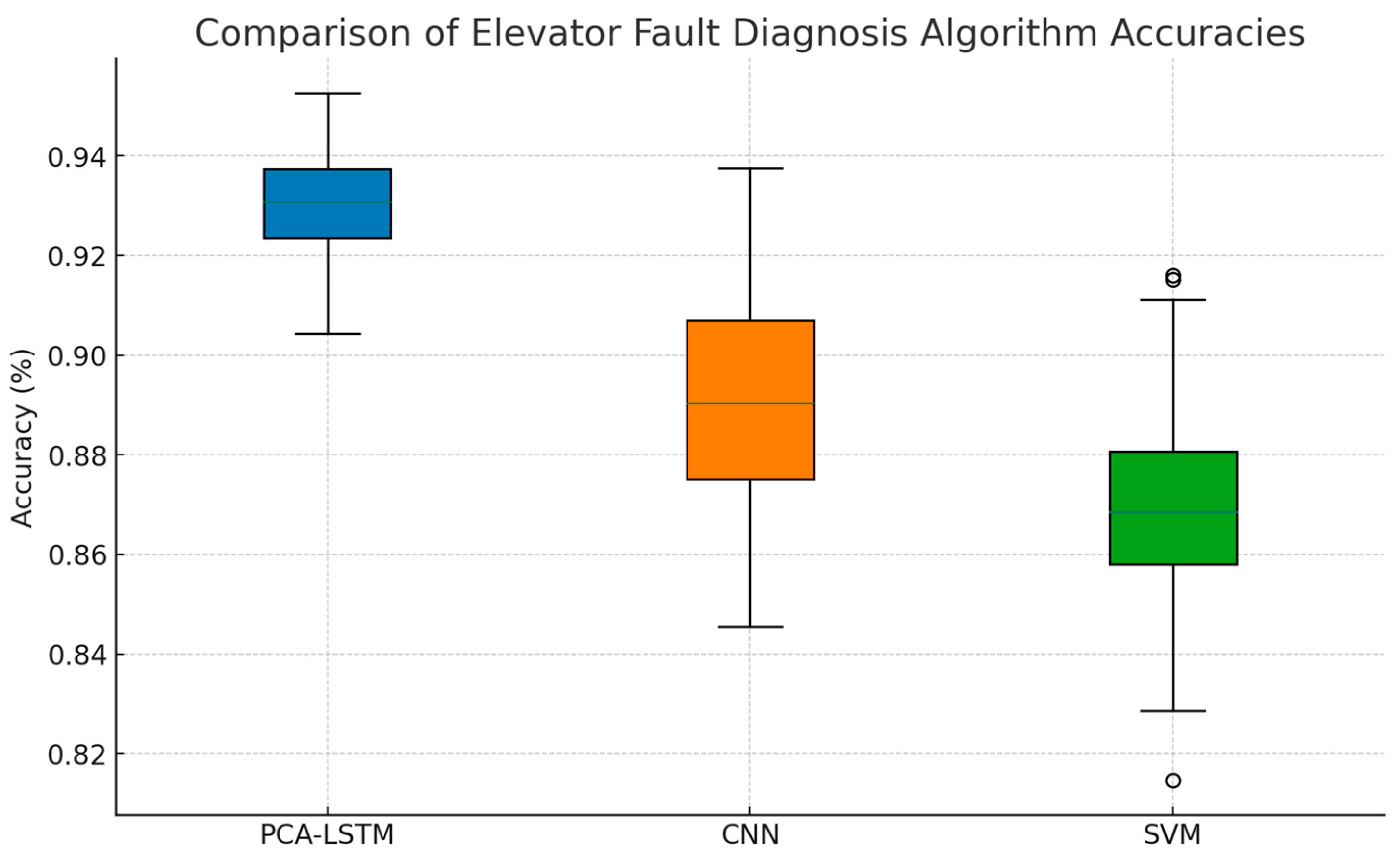
The second core idea focuses on distributed elevator fault diagnosis. Through experiments, the proposed fault prediction method achieves an accuracy of more than 90% in classifying the fault types of multiple elevators under the same working conditions, and the distributed technology enables local fault diagnosis within the elevator, which alleviates pressure on the central processor.

(3)

Currently, the distributed elevator fault diagnosis technique based on the PCA-LSTM model proposed in this paper delivers more satisfactory results in terms of spatial distribution. However, concerning model integration and parameter exchanges, the communication time between adjacent elevators is prolonged, which, in turn, increases the training time. Consequently, the speed of elevator parameter exchanges in the distributed scenario requires further consideration in future developments.

The implementation of distributed fault diagnosis systems for elevators presents several challenges inherent to their distributed nature. Firstly, synchronization issues arise, as data from various elevators must be aggregated and processed in real time to ensure timely fault detection. This necessitates robust algorithms capable of handling asynchronous data inputs without compromising the system’s responsiveness. Secondly, data privacy is a critical concern, as information collected from multiple elevators may contain sensitive user or operational data. Implementing stringent data protection protocols and secure data transmission mechanisms is essential to safeguard this information. Lastly, the scalability of models across multiple elevators is challenging, as the system must adapt to varying operational conditions and elevator architectures. Developing adaptive models that can generalize well across different setups while maintaining high diagnostic accuracy is crucial for the widespread applicability of these systems.

References

1. Lu, M.; Xie, Y.; An, Z. Elevator Error Diagnosis Method Based on Neural Network Model. In Proceedings of the 2023 International Conference on Network, Multimedia and Information Technology (NMITCON), Bengaluru, India, 1–2 September 2023; pp. 1–5. [Google Scholar] [CrossRef]
2. Liang, T.; Chen, C.; Wang, T.; Zhang, A.; Qin, J. A Machine Learning-Based Approach for Elevator Door System Fault Diagnosis. In Proceedings of the 2022 IEEE 18th International Conference on Automation Science and Engineering (CASE), Mexico City, Mexico, 20–24 August 2022; pp. 28–33. [Google Scholar] [CrossRef]
3. Zheng, B. Intelligent Fault Diagnosis of Key Mechanical Components for Elevator. In Proceedings of the 2021 CAA Symposium on Fault Detection, Supervision, and Safety for Technical Processes (SAFEPROCESS), Chengdu, China, 17–18 December 2021; pp. 1–3. [Google Scholar] [CrossRef]
4. Zhang, A.; Chen, C.; Wang, T.; Cheng, L. Fault diagnosis of Elevator Door Machines Based on Deep Convolutional Forest. In Proceedings of the 2022 27th International Conference on Automation and Computing (ICAC), Bristol, UK, 1–3 September 2022; pp. 1–6. [Google Scholar] [CrossRef]
5. Qiu, C.; Zhang, L.; Li, M.; Zhang, P.; Zheng, X. Elevator Fault Diagnosis Method Based on IAO-XGBoost under Unbalanced Samples. Appl. Sci. 2023, 13, 10968. [Google Scholar] [CrossRef]
6. Chen, Z. An elevator car vibration fault diagnosis based on genetically optimized RBF neural network. China Sci. Technol. Inf. 2023, 30, 110–115. [Google Scholar]
7. Liang, H.; Fushun, L.; Jie, L. Analysis of an elevator repeated door opening and closing fault using fault tree analysis. China Elev. 2023, 34, 71–73. [Google Scholar]
8. Cong, W.; Mengnan, L.; Kun, L. Elevator bearing fault detection based on PBO and CNN. Inf. Technol. 2023, 47, 73–78. [Google Scholar]
9. Li, Z.; Chai, Z.; Zhao, C. Abnormal vibration fault diagnosis of elevator based on multi-channel convolution. Control Eng. 2023, 30, 427–433. [Google Scholar]
10. Wei, Y.; Liu, H.; Yang, L. Fault diagnosis method of elevator traction wheel bearing based on angular domain resampling and VMD. Mech. Electr. Eng. 2023, 8, 1259–1266. [Google Scholar]
11. Jin, L.; Zhang, Z.; Shao, X.; Wang, X. Research on elevator fault identification method based on kernel entropy component analysis. Autom. Instrum. 2022, 39, 115–119. [Google Scholar]
12. Liu, Y.; Zhao, Y.; Wei, B.; Ma, T.; Chen, Z. Research on elevator fault diagnosis system based on optimization neural network. Autom. Instrum. 2022, 39, 88–92. [Google Scholar]
13. Dingsong, B.; Ziliang, A.; Ning, W.; Shaofeng, L.; Xintong, Y. The Prediction of the Elevator Fault Based on Improved PSO-BP Algorithm. J. Phys. Conf. Ser. 2021, 1906, 012017. [Google Scholar]
14. Chen, L.; Lan, S.; Jiang, S. Elevators Fault Diagnosis Based on Artificial Intelligence. J. Phys. Conf. Series 2019, 1345, 042024. [Google Scholar] [CrossRef]
15. Haoxiang, W.; Chao, L.; Dongxiang, J.; Zhanhong, J. Collaborative deep learning framework for fault diagnosis in distributed complex systems. Mech. Syst. Signal Process. 2021, 156, 107650. [Google Scholar]
16. Jan, S.U.; Lee, Y.D.; Koo, I.S. A distributed sensor-fault detection and diagnosis framework using machine learning. Inf. Sci. 2021, 547, 777–796. [Google Scholar] [CrossRef]
17. Murad, A.; Zakiud, D.; Evgeny, S.; Mehmood, C.K.; Ahmad, H.M.; Che, Z. Open switch fault diagnosis of cascade H-bridge multi level inverter in distributed power generators by machine learning algorithms. Energy Rep. 2021, 7, 8929–8942. [Google Scholar]
18. Qiu, S.; Cui, X.; Ping, Z.; Shan, N.; Li, Z.; Bao, X.; Xu, X. Deep Learning Techniques in Intelligent Fault Diagnosis and Prognosis for Industrial Systems: A Review. Sensors 2023, 23, 1305. [Google Scholar] [CrossRef] [PubMed]
Figure 1. Proportion of variance explained by principal components in elevator experiment data, justifying the 85% threshold.
Algorithms 17 00250 g001
Figure 2. Structure of the LSTM.
Algorithms 17 00250 g002
Figure 3. Structure flowchart.
Algorithms 17 00250 g003
Figure 4. Distributed deep learning framework for elevators.
Algorithms 17 00250 g004
Figure 5. Broadcast schematic diagram.
Algorithms 17 00250 g005
Figure 6. Data-parallel schematic diagram.
Algorithms 17 00250 g006
Figure 7. Diagnostic accuracy of distributed elevator fault detection systems.
Algorithms 17 00250 g007
Figure 8. Data schematic diagram after dimension reduction.
Algorithms 17 00250 g008
Figure 9. Performance of PCA-LSTM model in predicting elevator speed and fault detection.
Algorithms 17 00250 g009
Figure 10. Training and validation loss trends for PCA-LSTM elevator fault prediction model.
Algorithms 17 00250 g010
Figure 11. ROC curve of the PCA-LSTM model.
Algorithms 17 00250 g011
Figure 12. Comparison of PCA-LSTM’s accuracy compared to that of various algorithms.
Algorithms 17 00250 g012
Figure 13. Performance comparison of PCA-LSTM and IAO-XGBoost models across various elevator fault types.
Algorithms 17 00250 g013
Figure 14. Comparative analysis of PCA-LSTM and DBN models for elevator fault diagnosis.
Algorithms 17 00250 g014
Figure 15. Confusion matrix diagram.
Algorithms 17 00250 g015
Figure 16. F1 score plot.
Algorithms 17 00250 g016
Figure 17. Distributed model diagnosis effect diagram.
Algorithms 17 00250 g017