Abstract
Ballast serves a vital structural function in supporting railroad tracks under continuous loading. The degradation of ballast can result in issues such as inadequate drainage, lateral instability, excessive settlement, and potential service disruptions, necessitating efficient evaluation methods to ensure safe and reliable railroad operations. The incorporation of computer vision techniques into ballast inspection processes has proven effective in enhancing accuracy and robustness. Given the data-driven nature of deep learning approaches, the efficacy of these models is intrinsically linked to the quality of the training datasets, thereby emphasizing the need for a comprehensive and meticulously annotated ballast aggregate dataset. This paper presents the development of a multi-dimensional ballast aggregate dataset, constructed using empirical data collected from field and laboratory environments, supplemented with synthetic data generated by a proprietary ballast particle generator. The dataset comprises both two-dimensional (2D) data, consisting of ballast images annotated with 2D masks for particle localization, and three-dimensional (3D) data, including heightmaps, point clouds, and 3D annotations for particle localization. The data collection process encompassed various environmental lighting conditions and degradation states, ensuring extensive coverage and diversity within the training dataset. A previously developed 2D ballast particle segmentation model was trained on this augmented dataset, demonstrating high accuracy in field ballast inspections. This comprehensive database will be utilized in subsequent research to advance 3D ballast particle segmentation and shape completion, thereby facilitating enhanced inspection protocols and the development of effective ballast maintenance methodologies.
1. Introduction
According to the Association of American Railroads (AAR), freight railroads account for approximately 40% of the United States’ long-distance freight volume, with over one-third of the nation’s exports transported by rail []. The U.S. railroad infrastructure predominantly consists of ballasted tracks, where the track substructure plays a crucial role in overall performance. The ballast layer, a key component of the track substructure, provides essential structural support and facilitates drainage, directly influencing track strength, modulus, and deformation behavior. Ballast degrades and breaks down under repeated train loading. This can lead to poor drainage, track settlement, and reduced stability, and may also result in service interruptions and maintenance concerns. The use-related degradation of ballast is commonly referred to as “fouling” in railroad engineering practice. Evaluating ballast fouling levels is crucial for railroad inspection and maintenance []. The current methods for assessing ballast fouling conditions include visual inspection, field sampling with subsequent laboratory sieve analysis, and the use of Ground Penetrating Radar (GPR) []. However, visual inspection can be subjective [] and field sampling combined with laboratory sieve analysis is labor-intensive. Additionally, GPR data do not offer detailed information on ballast size and shape properties [,].
To address the deficiencies of current ballast evaluation methodologies, computer vision-based techniques have been proposed to enhance the reliability of infrastructure inspections. The advent of Vision Transformer (ViT) architectures [] has significantly enhanced the accuracy and reliability of ballast particle segmentation from 2D images compared to traditional Convolutional Neural Networks (CNNs). Luo et al. [] employed a Swin Transformer [], a hierarchical ViT framework with shifted windows, and Cascade Mask R-CNN [] and developed a well-tuned model for ballast instance segmentation. Leveraging advanced deep learning techniques, these ballast inspection systems are capable of providing near real-time evaluations in an automated manner, thereby enhancing the analysis of ballast conditions in field environments [].
Contrary to the segmentation of larger aggregate particles, the task of ballast segmentation is significantly more complex. It necessitates the detection and segmentation of much smaller particles from images obtained under challenging field conditions []. This complexity requires higher-quality datasets to train deep learning models, which in turn demands specialized image acquisition devices and hardware for field data collection []. Moreover, the annotation process—labeling the contours of ballast particles on images for model training—is both time-consuming and labor-intensive. Consequently, datasets composed of ballast images from field and laboratory sources remain limited in size and are difficult to scale effectively.
Data synthesis has been extensively employed to generate training datasets and improve the performance of machine learning (ML) models [,,,,]. Generative Adversarial Networks (GAN) [] utilize deep learning techniques to avoid complicated modeling and rendering designs and have been used to create synthetic data to assist railroad inspection in practice [,,]. These works usually require an input image as a reference and then apply GAN to generate an enhanced image [,] from the poor-quality input or to make the input fake image more similar to a real image. However, GAN models are relatively hard to train and require heavy computational resources, leading to a low-resolution output, typically of size 512 pixel × 512 pixel [], which can severely impact the detection of smaller ballast particles. On the other hand, to generate high-quality 2D synthetic images for ML purposes, 3D modeling software, such as Blender 2.5 [], is capable of precise modeling and realistic rendering, and has become another popular approach among recent studies [,]. Once the 3D models are established in the modeling software, different environmental lights, textures, camera orientations and parameters can be applied to the rendering procedure, providing much more flexibility to data synthesis.
This paper presents recent research initiatives aimed at overcoming the limitations of existing ballast datasets, which comprise images from both field and laboratory settings, by integrating an augmented dataset specifically for ballast segmentation and evaluation. The newly developed database encompasses all well-annotated field ballast images utilized in prior studies by the research team [,] and is further enhanced with a significant volume of synthetic data generated by a popular 3D modeling tool, Blender, through a custom automated workflow. The augmented dataset, enriched with synthetic ballast data, has undergone experimental validation to facilitate the development of more advanced and effective deep learning models.
2. Objective and Scope
The objective of this research effort was to demonstrate how deep learning methods developed to perform field ballast condition analysis using high-quality real ballast data collection can be further improved through synthetic ballast data generation and dataset augmentation. This paper first describes how to collect and annotate high-quality images of real ballast from both the field and laboratory. It then introduces a synthetic ballast data generation pipeline, and a synthetic ballast dataset established with the proposed pipeline. The validation of the proposed synthetic ballast dataset was accomplished through deep learning models trained with comparable performances in the task of field ballast image segmentation and how they compare to models trained with datasets of actual ballast samples only. This paper finally demonstrates how an augmented ballast dataset combining both real and synthetic ballast data can enhance the segmentation performance.
3. Field and Lab Ballast Data Preparation
3.1. Overview
The selection criteria for the ballast images in the dataset were rigorously defined to ensure comprehensive coverage: (i) inclusion of ballast images obtained from diverse railroad field sites as well as laboratory environments; (ii) representation of a wide range of ballast sources, encompassing particles of different sizes, colors, and textures; and (iii) inclusion of images captured under various lighting conditions and exhibiting different levels of degradation. Table 1 provides a summary of the sources and fouling conditions for the ballast images incorporated into the dataset.

Table 1.
Ballast image dataset collected from railroad field and laboratory setups [].
3.2. Methodology
3.2.1. Field Data Acquisition
Ballast images obtained from a variety of field sites introduce different ballast types and field conditions to the dataset. In total, 144 field ballast images were collected from six distinct railroad sites, including the Transportation Technology Center (TTC) High Tonnage Loop (HTL) in Pueblo, Colorado; Burlington Northern Santa Fe (BNSF) track near Kansas City, Missouri; Union Pacific (UP) track in Martinton, Illinois; Canadian National (CN) track in Champaign, Illinois; Norfolk Southern (NS) track in Champaign, Illinois; NS track near Sandusky, Ohio; and NS track near Kendallville, Indiana. These field images encompass a variety of ballast characteristics including type, color, degradation level, size distribution, and particle arrangement. Field ballast images from railroad field sites were collected with a self-invented Ballast Scanning Vehicle (BSV) equipped with a line scan camera and an area scan camera in an automated manner []. Additionally, aggregate images sourced from various aggregate producers (i.e., quarries) serve as a supplementary contribution, enhancing the dataset’s inclusivity. These images depict clean aggregate stockpiles comprising medium- to large-sized particles, which are either slightly separated or densely stacked. Images from aggregate quarries were collected with smartphone cameras, and detailed camera settings were introduced in the previous work [].
3.2.2. Laboratory Data Collection
To comprehensively examine how various field conditions impact image segmentation performance, five pivotal influencing factors are considered: particle size, color, arrangement (i.e., the packing and overlapping of particles), lighting conditions, and degradation levels. Analyzing ballast images with diverse field conditions proves challenging due to the difficulty in precisely identifying the dominant factor(s) affecting segmentation performance. In uncontrolled field environments, isolating these factors for study is impractical. Consequently, capturing images of ballast particles in a well-controlled environment in the laboratory is important for giving clear guidance in training the ballast particle segmentation models. The approach facilitates the examination of different permutations of the five key variables and enhances the dataset’s comprehensiveness.
For laboratory images, three types of ballast materials were prepared: (i) white limestone, (ii) dark red quartzite, and (iii) dark gray igneous rock (basalt or granite). Each material was divided into four distinct particle size groups based on AREMA ballast gradation specifications: (i) particles passing the 3/8 in. (9.53 mm) sieve, indicating fouled materials and fines; (ii) particles retained on the 3/8 in. (9.53 mm) sieve; (iii) particles retained on the 1 in. (25.4 mm) sieve; and (iv) particles retained on the 2 in. (51 mm) sieve. To ensure diverse coverage, various ballast particle configurations were designed to account for different combinations of the critical influencing factors.
The complexity of particle configurations ranged from single-size groups in a non-contacting setting, to mixed-size groups/mixed colors, and eventually full gradations. Different lighting conditions were introduced, spanning from direct natural sunlight to shaded or diffused lighting, mirroring potential field lighting conditions. All images were captured perpendicular to the stockpile surface/ballast particles using a tripod with a cantilever arm and a smartphone camera. For each configuration, two images were taken at two heights (30 in. (762 mm) and 45 in. (1143 mm)). Additionally, a 1.5 in. (38.1 mm) diameter white ball was employed for scale calibration.
3.2.3. Data Processing and Labeling
The “image labeling” or “image annotation” step is critical for providing accurate information to the segmentation kernel during training. This step involves marking the locations and regions of all ballast particles that are discernible to the human eye in each image. The quality of the labeling directly impacts the segmentation kernel’s performance, and the process can be time-consuming and labor-intensive. Each particle region was annotated with two key components: (i) a polygon intended to overlap with the detected particle region and (ii) an object class label—in this study, “ballast”—to categorize the type of segmented particle. By assimilating these components, the deep neural network can learn the intrinsic features of existing particles and develop predictive capabilities to automate the detection and extraction of ballast particles from given images.
For this task, VGG Image Annotator (VIA) [], an open-source manual annotation software for image, audio, and video, was selected out of the other widely used image annotation tools, such as LabelMe [] and Computer Vision Annotation Tool (CVAT) [], to aid the labeling process. VIA is based solely on Hypertext Markup Language (HTML), JavaScript, and Cascading Style Sheets (CSS), thus running simply in a web browser without any additional requirements for installation or setup. VIA’s lightweight characteristics make it possible to create many annotations (over 500 particles per image) on high-quality images of large resolutions smoothly with limited computational and storage resources. This ballast particle annotation task did not apply artificial intelligence (AI)-assisted image labeling techniques [] as pretrained segmentation models used in existing AI-assisted annotation tools failed to provide delicate labels for ballast particles thus requiring heavy manual refinement. During manual ballast image labeling, a set of criteria was adopted to standardize the process and ensure the quality of annotations: (i) all particles that can be identified visually should be labeled with a high-resolution polygon describing their boundaries in details; (ii) if particles contain straight edges at the image boundary, these edges should be split into multiple shorter line segments to maintain polygonal detail; and (iii) polygons with more edges should be favored to accurately represent the boundaries of smoother particles.
According to the proposed process of the image acquisition and annotation, a ballast image dataset comprising 423 images with ground-truth labels was established.
4. Synthetic Data Generation
4.1. Overview
The dataset comprising images of actual ballast particles has demonstrated its effectiveness in building and training deep learning models for 2D ballast particle segmentation in field images. Nevertheless, the dataset has the following limitations:
- Limited accessibility. Acquiring a high-quality ballast dataset for training robust deep learning models requires access to dedicated in-service railroad sites, high-end equipment, and coordination with specialized departments with domain knowledge.
- Limited scalability. The processes of gathering, processing, and annotating field data are time-consuming and labor-intensive.
- Limited flexibility. Extracting specific forms of data, such as individual ballast particles within a 3D reconstructed point cloud, can be extremely challenging and may be unattainable from images of actual ballast in real-world scenarios.
To overcome these limitations, a synthetic ballast dataset was established with support from Blender 3D modeling software. This supplemental ballast dataset is accessible, scalable, flexible, and capable of augmenting the existing actual ballast image datasets with high-quality synthetic ballast images to enhance the performance of the deep learning models in the task of ballast particle segmentation from field-collected images.
The synthetic ballast dataset is structured around “scenes” as its primary unit of analysis. Each scene represents an individual sample of ballast aggregate, encompassing all necessary information to generate comprehensive synthetic ballast data and annotations. This methodology obviates the need for the labor-intensive manual labeling process by automating it. The synthetic dataset consists of 120 generated scenes, each containing hundreds of ballast particles. These particles display a range of sizes, shapes, and textures, adhering to an assigned gradation distribution. Each scene is composed of three principal elements: ballast data, ballast labels, and statistical information that characterizes the ballast data (as illustrated in Figure 1).
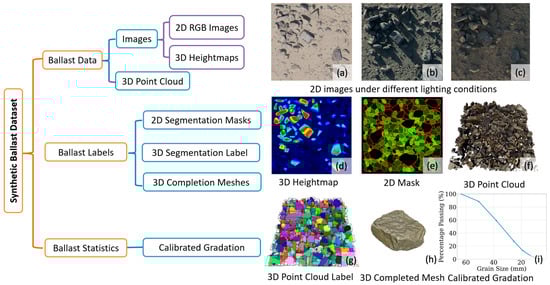
Figure 1.
Components in synthetic ballast dataset. Left: Architecture of the synthetic ballast dataset. Right: Examples of various data categories within the synthetic ballast dataset []. (a–c) 2D synthetic ballast images under different lighting conditions. (d) 3D heightmap. (e) Masks of ballast particles for 2D synthetic ballast images. (f) 3D point cloud of ballast particles. (g) Labels of ballast particles for 3D ballast point clouds, each 3D point is rendered in a specific color that indicate the ballast particle it belongs to. (h) 3D completed mesh of a ballast particles. (i) Ballast particle size distribution curve.
- Ballast data. The ballast dataset provides high-resolution (2500 pixel × 2500 pixel) RGB images captured from a top-down perspective under various lighting conditions (Figure 1a–c). It also contains a 3D heightmap (Figure 1d) corresponding to the base plane, a 3D textured point cloud (Figure 1f) encompassing all the ballast particles within the scene, and individual, complete meshes for each ballast particle. Figure 1d visualizes the generated 3D heightmap, where the height of each pixel to the base plane is encoded with a colormap ranging from dark blue to red, where red pixels indicate the highest points in the physical world. The diversity of the synthetic data allows for the emulation of a wide range of commonly used ballast imaging devices, including but not limited to line scan cameras, area scan cameras, and 3D laser scanners.
- Ballast labels. Within a generated scene, each synthetic ballast particle is assigned a unique particle ID ranging from 1 to the number of particles in the scene. The label of a synthetic 2D ballast image (2D particle masks) paired with the ballast data is a map from each pixel in the 2D ballast image to its corresponding ballast particle’s unique ID. Figure 1e visualizes the 2D particle mask for a top-view RGB image, where the red polygons are the outlines of each ballast particle, and the color of each pixel inside the red polygons encodes its unique ballast particle ID. Similarly, the label of a generated 3D ballast point cloud is a map from each 3D point in the point cloud to its corresponding ballast particle’s unique ID. Figure 1g visualizes the label of a 3D point cloud by rendering each point in the point cloud with a unique color encoding its unique ballast ID, indicating that points with the same color belong to the same ballast particle. The gray cuboids in Figure 1g show the 3D bounding box of each ballast particle. Furthermore, from the unique particle ID, the completed mesh (Figure 1h) that each 3D point belongs to can be linked. These auto-generated annotations allow multi-dimensional ballast instance recognition and segmentation.
- Ballast statistics. In practice, statistical aggregate features can provide valuable insights into the geotechnical characteristics of the ballast sample, like fouling conditions. Therefore, the actual particle size distribution (PSD) (Figure 1i), as well as a series of morphological metrics including sphericity, the flat and elongated ratio (FER), and angularity for particles over 3/8 in. (9.5 mm), is calculated and appended for each generated scene.
Table 2 outlines the scope of the synthetic dataset. To replicate ballast samples in various fouling conditions, the generation of scenes is managed by a series of particle size distributions (PSDs) corresponding to different Fouling Index (FI) values. Given that the dataset can be automatically produced by a synthetic data generation pipeline without human intervention, it possesses substantial scalability potential.
Table 2.
Overview of the generated synthetic ballast image dataset [].
The methodology employed for preparing ballast particle meshes, simulating the physical scene, creating realistic images, and generating instance annotations, is explained in the following sections.
4.2. Three-Dimensional Mesh Libarary of Actual Ballast Particles
The first step is to obtain several 3D digital models of actual ballast particles for synthetic scene generation. A 3D laser scanner (Figure 2, manufactured by Roland, Hamamatsu, Japan) was used to measure, calculate, and export the 3D meshes of actual ballast particles collected from the same sources as those used for the acquisition of laboratory ballast images. As a result, a 3D ballast library containing 120 high-fidelity models for ballast particles collected from different sources was obtained.
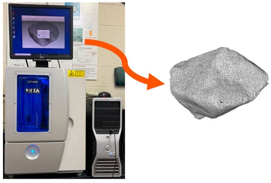
Figure 2.
Three-dimensional laser scanner used to scan the ballast particles and export their 3D meshes.
Ballast particle shape, texture, and angularity significantly impact the railroad track mechanical behavior. Since the synthetic ballast dataset is used to train models with computer vision tasks including ballast particle segmentation and completion, the obtained 3D ballast library should contain various morphological characteristics to resemble the different shapes of actual ballast particles. To validate the shape diversity of the scanned meshes, three morphological indicators were introduced: 3D flat and elongated ratio () [], 3D sphericity [], and 3D angularity index () [].
The 3D FER, defined in Equation (1), is the ratio of the longest Feret dimension to the shortest Feret dimension of the 3D ballast particle:
where are the lengths of three Feret dimensions for the particle.
The 3D sphericity, as expressed in Equation (2), is defined as the ratio of , the surface area of an equivalent sphere with the same volume, , as the particle, to , the measured surface area of the particle. It can indicate whether the ballast is close to a perfect sphere.
The 3D AI, as expressed in Equation (3), is defined as the ratio of , the measured surface area of the particle, to , the surface area of an equivalent ellipsoid with the same volume, , as the particle and the same proportion of long, middle, and short axes.
Figure 3 illustrates the dispersion of scanned ballast models based on three morphological indicators. The distribution of these scanned particles encompasses a wide variety of shapes, effectively mitigating any shape-related biases. Each figure displays particle shapes alongside their respective minimum, intermediate, and maximum indicator values.
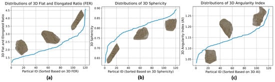
Figure 3.
Morphological characteristics of the scanned meshes of individual ballast particles. Distributions of (a) 3D flat and elongated ratio (FER), (b) 3D sphericity, and (c) 3D angularity index (AI) [].
4.3. Scene Simulation and Ballast Data Rendering
To guarantee that the generated digital scene accurately represents real-world ballast samples encountered in the field, a robust physics simulation and rendering workflow were meticulously designed, illustrated in Figure 4.
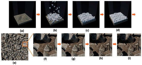
Figure 4.
Generation of synthetic ballast data. (a) Initialize base container. The bottom of the container is 3.3 ft × 3.3 ft (1 m × 1 m), and the transparent walls of the container are 6.6 ft (2 m) in height. (b) Generate particles >3/8 in. (9.5 mm) according to the input particle size distribution (PSD) and freely release them from random locations inside the container without overlapping under gravity. (c) Shake the container by periodically changing the direction of the gravity to ensure uniform mixing of the ballast particles. (d) Calculate the height of the fine surface according to the input PSD, then add the fine surface of the same size as the bottom of the container to the scene. (e) Place a camera to visualize the plan view of the ballast scene and assign random textures to the ballast particles and fine material surface. (f) An enlarged view of the image (e). (g) Add ballast particles in sizes of 0.1~3/8 in. (2.54~9.5 mm) on top of the fine material surface to better resemble real ballast sizes in the field. (h) Mix textures of the fine material and the ballast particles to mimic the appearance of field ballast particles covered with fine materials. (i) Add ballast particles in sizes of 0.03~0.1 in. (0.762~2.54 mm) on top of the fine material surface with a hair particle system [].
4.3.1. Physical Simulation
The physical simulation was performed using Blender software [], which internally adopts the Bullet physics engine [], a free and open-sourced development kit for real-time collision detection and multi-physics simulation.
Ballast particles in a railroad track lie stably on the underlying sub-ballast or subgrade layer under the effects of gravity. Under repeated train loading, ballast particles will degrade and may break into smaller particles. Therefore, the particle size distribution (PSD) indicates the fouling condition of the ballast.
The shape of each ballast particle within the scene was randomly selected from the prepared meshes of 120 ballast particles. Each scene was assigned a target number of ballast objects (in the range of 400~600), and these ballast objects were properly scaled to satisfy the target PSD, to simulate various fouling conditions. Since applying physics simulation on such a number of objects with sophisticated meshes can be extremely resource-intensive, the ballast objects were represented by a simplified mesh (~100 facets left) with the decimation algorithm [] until final rendering, a trade-off between precision and efficiency.
When the simulation started, ballast particles over 3/8 in. (9.5 mm) first started free-falling from different random heights without overlapping (Figure 4b) to a 3.3 ft × 3.3 ft (1 m × 1 m) sub-ballast or subgrade plane surrounded by transparent walls of 6.6 ft (2 m) in height (Figure 4a) to prevent ballast particles from falling out. However, free-falling tends to make the smaller particles settle down to the bottom through vacancies. To mix all sizes evenly, the virtual container was shaken by periodically changing the direction of gravity (Figure 4c).
Considering the large quantities of ballast particles and the simulation precision, it is exceptionally challenging to simulate fine materials with the same approach. Thus, only the surface of the fine materials was added to the scene (Figure 4d). The height of the fine materials surface, , was cautiously calculated so that the mass of the fine materials satisfies the input PSD. The net volume of the fine materials, , is calculated by
where is the vacant space underneath the surface of the container (excluding ballast particles over 3/8 in. (9.5 mm)), and is the porosity of the fine material [].
To make the fine material surface more realistic, 400 to 600 randomly picked smaller ballast particles, with sizes uniformly sampled in the range from 0.1 in. (2.54 mm) to 3/8 in. (9.5 mm), underwent free-falling to the fine material surface (Figure 4g). After all smaller ballast particles stayed still, the height of the fine material surface was adaptively adjusted to obey the input particle size distribution. Smaller particles of sizes 0.03~0.1 in. (0.762~2.54 mm) were made to adhere to the fine material surface using a hair particle system due to the large quantities. A hair particle system in Blender can manage up to 10,000,000 particles emitted from mesh objects efficiently and perform fast rendering (Figure 4i).
4.3.2. Rendering
The data generation pipeline enters the rendering stage after the physical scene is fully simulated and every object within the scene is in a stable status. The rendering engine used is Cycles [], Blender’s physical-based path tracer for product rendering. A new rendering technique, adaptive texture mixing, was designed and adopted to make the scene renders more natural and closer to the field-collected images. This technique was used in addition to regular rendering techniques, such as smart UV mapping for fitting the same texture to different objects, adjustable environment mapping for lighting condition randomization, and bumps and displacements [] for realistic terrain surface rendering.
Before rendering, each ballast particle together with the fine material surface was assigned a random texture selected from a human-pre-screened texture library, which included 25 textures for the ballast particles and 38 textures for the fine material. A direct rendering with the assigned textures would result in unnatural outcomes (Figure 4e–g), because in real-world scenarios, ballast particles would seldom be clean on the surface. Fine materials would adhere to the surface of the ballast particles, especially under the effect of moisture. Thus, an adaptive texture mixing approach was designed to serve this purpose (Figure 4h).
When employing adaptive texture mixing, the texture of ballast particles was combined with that of the fine material through a randomly generated noise mask, guided by input parameter ‘r’. This parameter ‘r’ is related to the percentage of the particle surface area covered by fine materials. Figure 5 illustrates the progressive alteration in the rendering of a ballast particle as ‘r’ increases during the texture-mixing step depicted in Figure 4h.
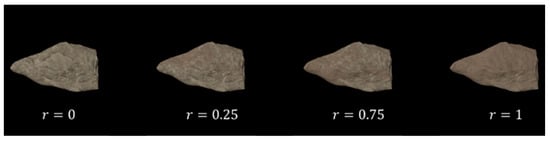
Figure 5.
Synthetic ballast particles in adaptively mixed textures with different ‘r’ values [].
The implementations for the adaptive texture mixing can vary, as long as they ensure the rule that a larger parameter ‘r’ results in a larger rate at which the ballast particle surface is covered with fine materials. Equation (5) shows an example implementation of the adaptive texture mixing used for Figure 5:
where is a randomly generated noise mask taking input point coordinate and providing a random number ranging from 0 to 1. The result, of Equation (5), ranging from 0 to 1, stands for the texture mixing rate of the point ‘c’ under the input parameter ‘r’. Then, the final texture of point ‘c’ in the output image will result in a mix of coarse ballast texture and fine material texture , following Equation (6) during rendering.
During synthetic ballast generation, larger ‘’ values were assigned to ballast scenes exhibiting higher fouling conditions, thereby more accurately mirroring the appearance of field ballast.
Figure 6 presents examples of synthetic ballast images generated by the proposed rendering method with different configurations of light conditions, particle size distributions, and textures of ballast particles and fine material surfaces.
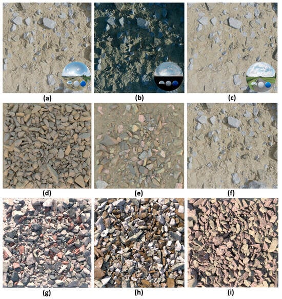
Figure 6.
Examples of synthetic ballast images with: (a–c) different light conditions, (d–f) different particle size distributions, and (g–i) different textures of ballast particles and fine material surface.
4.4. Dataset Acquisition from the Generated Scenes
After generating the scenes, ballast data and the corresponding labels were prepared in an automated fashion. Using Blender’s Compositing Nodes, rendering graphs can be built at runtime, enabling rendering multiple information acquired from the same camera view, such as RGB images, depth maps, and visible object indices. The output data are aligned with inputs and can be flexibly encoded and exported to multiple image formats, based on the required precision. The proposed automated procedures for obtaining both 2D and 3D synthetic datasets are built on top of this feature.
4.4.1. Two-Dimensional Images and Masks
The 2D ballast images and masks of each ballast particle were collected in a straightforward manner by rendering RGB colors and visible object indices as two outputs, which were assigned prior to rendering using Compositing Nodes. Unique object indices should be assigned to the objects of interest before rendering. In terms of the output image formats, object indices can either be encoded into integer vectors and stored in the RGB channel to be saved as PNG images with no compression or may be converted to float scalars and exported as single-channel EXR images.
In the synthetic ballast dataset, the objects of interest are ballast particles of sizes larger than 3/8 in. (9.5 mm). In practice, some ballast particles might be blocked by other ballast particles or fines on the surface, resulting in some particle masks being too small or broken into disconnected pieces. Therefore, the post-processing of the saved object index maps to filter out these masks is essential to ensure the training effectiveness. The cleaned 2D dataset is then packed into the widely used COCO dataset format [] for better training compatibility.
4.4.2. Three-Dimensional Point Cloud and Annotations
Blender software provides tools to export point clouds from meshes in the scene. However, common aggregate point clouds are either collected by 3D scanners or reconstructed from a set of multi-view 2D RGB images, both of which are incapable of containing invisible object points in the output point clouds. To obtain scanned/reconstructed 3D point clouds, rendering was conducted from multiple camera perspectives, each producing three outputs: RGB colors (Figure 7a), object index map (Figure 7b), and depth map (Figure 7c). The depth map output format should be single-channel EXR images to retain the precision of 3D coordinates.
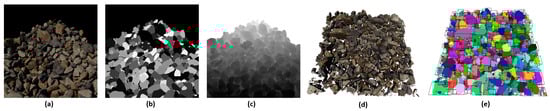
Figure 7.
Data collected from various camera perspectives include: (a) color image, (b) 2D segmentation labels (object indices), and (c) depth map. Through projecting all captured data into the world coordinate system, (d) the ground truth point cloud and (e) the 3D ground truth labels (different colors indicate different ballast particles) are obtained [].
When the rendering is completed, camera parameters are retrieved from each view to perform an inverse projection of 2D pixels from the color image and object index map back into 3D world coordinates using the depth map. This approach facilitates the generation of a textured point cloud (Figure 7d) and its corresponding annotations (Figure 7e). Within the output dataset, each 3D point within the point cloud is stored in a 10-dimensional array describing its 3-dimensional location in the world coordinate system, 3-dimensional RGB colors, 3-dimensional normal direction computed from depth maps, and the identification of the associated ballast particle as a 1-dimensional integer.
5. Evaluation of Results
The evaluation of synthetic datasets typically revolves around two primary criteria: fidelity and utility [,]. Fidelity [] describes the relevance of the generated synthetic data. For 2D synthetic images, fidelity can be understood as the similarity between the synthetic images and the real images, achieved by the proposed workflow for realistic scene generation and rendering. Utility [], on the other hand, measures how the synthesized dataset benefits fundamental computer vision tasks during ML model training. As fidelity is not straightforward to quantify, the evaluation focuses mainly on utility. To validate the utility of the generated synthetic ballast image dataset, several experiments were designed and conducted. The UIUC HAL Cluster provided all the computing resources necessary for training and testing the deep learning models used in these experiments [].
5.1. Comparison between Train on Real Test on Real (TRTR) and Train on Synthetic Test on Real (TSTR)
To evaluate the utility of the synthetic dataset, researchers [,,,] trained two ML models using the real and synthetic datasets and subsequently tested the trained models with a reserved subset of the actual ballast dataset that was not utilized during training. Various performance metrics, including accuracy, precision, and F1-Score, were employed to examine the variations in model performance []. Metrics for models trained on the real dataset were labeled as Train on Real Test on Real (TRTR), while those for models trained on the synthetic dataset were labeled as Train on Synthetic Test on Real (TSTR). If the TSTR metrics closely align with the TRTR metrics, the synthetic ballast dataset is considered effective for training models applicable to real-world scenarios.
Figure 8a provides a detailed illustration of the configuration of the experiment and its execution flow. Two distinct training datasets of ballast images were created to independently train a ballast segmentation model (Cascade Mask R-CNN with a Swin- Transformer as the backbone []) using identical network configurations. The first dataset included a subset of collected real ballast images, as described in Section 3, comprising 325 images with a total of 50,461 ballast particle instances. The second dataset consisted of a subset of synthetically generated ballast images, detailed in Section 4, containing 325 images with a total of 128,139 particles. After 36 training epochs, both segmentation models were tested using the same ballast dataset, which was randomly selected from the real-image dataset and not included in the training sets. This reserved real dataset comprised 22 images with 3505 ballast particles and was used as the testing dataset to assess and compare the performance of the two models after training.
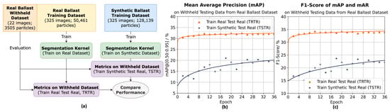
Figure 8.
Comparison between TRTR and TSTR. (a) Experimental flowchart. (b) Mean average precision () comparison. (c) F1-Score for and mean average recall () comparison [].
Additionally, among all experiments conducted, a series of traditional dataset augmentation techniques, including random flipping, random mirroring, random resizing to multiple preset aspect ratios, and random cropping, were applied to each input image while training all ballast particle segmentation models to be evaluated in this study.
The metrics employed to evaluate the performances of TRTR and TSTR include their mean average precision (, Figure 8b), mean average recall (), and F1-Score (Figure 8c), which are standard measures in the evaluation of image segmentation models [,]. The results demonstrate that although the model trained on the real dataset ( = 32.1%, = 34.3%) exhibits superior performance compared to the model trained on the synthetic dataset ( = 21.2%, = 23.9%), the metrics remain sufficiently comparable. This suggests that synthetic images can be utilized to effectively train models for ballast particle segmentation, notwithstanding the performance gap between real and synthetic data.
5.2. Comparison between Train on Real Test on Real (TRTR) and Train on Augmented Test on Real (TATR)
Alternatively, research conducted by Che et al. [], Wang et al. [], and Yang et al. [] evaluated synthetic data by training models on an augmented dataset with both real and synthetic data, subsequently comparing the performance to models trained solely on real data.
Figure 9 illustrates the experimental design for validating ballast segmentation models with augmented data. In addition to the datasets utilized in the prior experiment, a new augmented dataset combining real and synthetic training images was developed for this study. The experimental results reveal that the model trained on the augmented dataset ( = 32.9%, = 34.6%) surpasses the performance of the model trained exclusively on real data ( = 32.1%, = 34.3%). This enhancement indicates that augmenting the real ballast dataset with synthetic ballast data in training improves the model’s segmentation performance, thereby confirming the utility of the generated synthetic ballast images.
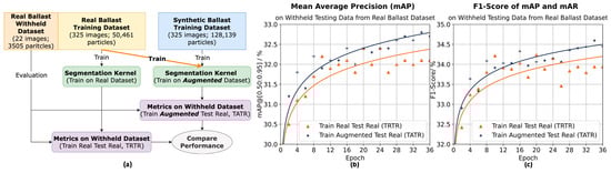
Figure 9.
Comparison between TRTR and TATR. (a) Experimental flowchart. (b) Mean average precision () comparison. (c) F1-Score calculated from and mean average recall () comparison [].
When comparing the segmentation results of models trained on the real dataset to those trained on the augmented dataset (Figure 10), it is evident that the segmentation kernel trained with the augmented datasets demonstrates superior performance. This enhancement is particularly pronounced when ballast particles are partially obscured by fine material, likely attributed to the adaptive texture-mixing technique applied during the synthetic scene rendering.
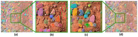
Figure 10.
Segmentation results on a real ballast image. (a) Ballast segmentation results obtained from the model trained exclusively on real ballast images and (b) zoom-in view. (c) Ballast segmentation results derived from the model trained using augmented ballast images and (d) zoom-in view. Different colors indicate different ballast particles detected.
Table 3 summarizes the evaluation metrics on the real ballast test dataset for all three models trained among the experiments. The augmented ballast dataset combining both real and synthetic ballast data could clearly enhance the segmentation performance.
Table 3.
Evaluation metrics on the real ballast test dataset for models trained with real ballast dataset (TRTR), synthetic ballast dataset (TSTR), and augmented ballast dataset (TATR).
6. Summary and Conclusions
This study introduces an augmented dataset that integrates both real and synthetic ballast data to improve the performance of deep learning models in the segmentation and evaluation of railroad ballast images. Details on the collection, processing, and annotation of the real ballast dataset were presented first in the paper, demonstrating how a high-quality real ballast image dataset could be established to effectively train deep learning models in practical applications.
To address the inherent limitations of relying solely on real ballast data, an automated workflow for synthesizing ballast data was developed. Two distinct experiments were carried out to assess the effectiveness of the synthetic ballast dataset, which was generated using specific scene generation and realistic rendering techniques. Nevertheless, the segmentation model trained solely with the synthetic ballast dataset underperformed that trained with the real dataset, indicating that gaps existed between the real data and generated synthetic data. To fill such gaps, it was worth investigating how the current data synthesis workflow could be improved, especially through integrating advanced techniques like domain randomization []. There are also opportunities to apply deep learning-based data augmentation methods, such as GANs [], to make the fake images more similar to the real field images. This progress can be crucial for future research studies that rely on synthetic datasets. Conversely, segmentation models trained on the augmented dataset—comprising both real and synthetic data—demonstrated improved precision and enhanced capabilities beyond those trained solely on real data. This approach underscores the advantages of integrating synthetic data to augment real datasets for improving model performance.
The proposed workflow for synthesizing ballast data also sets the stage for future research endeavors, including the development of 3D models for ballast particle segmentation, shape completion, and morphological analysis. These advancements aim to support more effective ballast inspection and investigative methodologies to facilitate optimal ballast maintenance strategies.
Author Contributions
The authors confirm their contribution to the paper as follows: conceptualization, E.T., J.M.H., K.D., J.L., H.H. and I.I.A.Q.; data collection, K.D., J.L., H.H. and J.M.H.; methodology, K.D.; validation, K.D.; writing—original draft preparation, K.D.; writing—review and editing, K.D., I.I.A.Q., E.T., J.M.H., J.L. and H.H.; supervision, E.T. and J.M.H.; funding acquisition, E.T. All authors have read and agreed to the published version of the manuscript.
Funding
This research received no external funding.
Data Availability Statement
The raw data supporting the conclusions of this article will be made available by the authors on request.
Acknowledgments
The authors would like to acknowledge the China Scholarship Council (CSC) scholarship, which provided funding for Kelin Ding’s time and research effort in this paper. The contents of this paper reflect the views of the authors who are responsible for the facts and the accuracy of the data presented. This paper does not constitute a standard, specification, or regulation.
Conflicts of Interest
The authors declare no conflicts of interest. The funders had no role in the design of the study; in the collection, analyses, or interpretation of data; in the writing of the manuscript; or in the decision to publish the results.
References
- Freight Rail & Climate Change–AAR. Available online: https://www.aar.org/issue/freight-rail-climate-change/ (accessed on 13 February 2024).
- Al-Qadi, I.L.; Rudy, J.; Boyle, J.; Tutumluer, E. Railroad Ballast Fouling Detection Using Ground Penetrating Radar—A New Approach Based on Scattering from Voids. e-J. Nondestruct. Test. 2006, 11, 8. [Google Scholar]
- Stark, T.D.; Wilk, S.T.; Swan, R.H. Sampling, Reconstituting, and Gradation Testing of Railroad Ballast. Railr. Ballast Test. Prop. 2018, 2018, 135–143. [Google Scholar] [CrossRef]
- Al-Qadi, I.L.; Xie, W.; Roberts, R. Scattering Analysis of Ground-Penetrating Radar Data to Quantify Railroad Ballast Contamination. NDT E Int. 2008, 41, 441–447. [Google Scholar] [CrossRef]
- Jol, H.M. Ground Penetrating Radar Theory and Applications; Elsevier: Amsterdam, The Netherlands, 2008; ISBN 978-0-08-095184-3. [Google Scholar]
- Dosovitskiy, A.; Beyer, L.; Kolesnikov, A.; Weissenborn, D.; Zhai, X.; Unterthiner, T.; Dehghani, M.; Minderer, M.; Heigold, G.; Gelly, S.; et al. An Image Is Worth 16 × 16 Words: Transformers for Image Recognition at Scale. arXiv 2020, arXiv:2010.11929. [Google Scholar]
- Luo, J.; Huang, H.; Ding, K.; Qamhia, I.I.A.; Tutumluer, E.; Hart, J.M.; Thompson, H.; Sussmann, T.R. Toward Automated Field Ballast Condition Evaluation: Algorithm Development Using a Vision Transformer Framework. Transp. Res. Rec. 2023, 2677, 423–437. [Google Scholar] [CrossRef]
- Liu, Z.; Lin, Y.; Cao, Y.; Hu, H.; Wei, Y.; Zhang, Z.; Lin, S.; Guo, B. Swin Transformer: Hierarchical Vision Transformer Using Shifted Windows. In Proceedings of the IEEE/CVF International Conference on Computer Vision (ICCV), Computer Vision (ICCV), Montreal, QC, Canada, 10–17 October 2021; pp. 9992–10002. [Google Scholar] [CrossRef]
- Cai, Z.; Vasconcelos, N. Cascade R-CNN: High Quality Object Detection and Instance Segmentation. arXiv 2019, arXiv:1906.09756. [Google Scholar] [CrossRef]
- Luo, J.; Ding, K.; Huang, H.; Hart, J.M.; Qamhia, I.I.A.; Tutumluer, E.; Thompson, H.; Sussmann, T.R. Toward Automated Field Ballast Condition Evaluation: Development of a Ballast Scanning Vehicle. Transp. Res. Rec. 2023, 2678, 24–36. [Google Scholar] [CrossRef]
- Wu, X.; Liang, L.; Shi, Y.; Fomel, S. FaultSeg3D: Using Synthetic Data Sets to Train an End-to-End Convolutional Neural Network for 3D Seismic Fault Segmentation. Geophysics 2019, 84, IM35–IM45. [Google Scholar] [CrossRef]
- Lalaoui, L.; Mohamadi, T.; Djaalab, A. New Method for Image Segmentation. Procedia-Soc. Behav. Sci. 2015, 195, 1971–1980. [Google Scholar] [CrossRef]
- Barth, R.; IJsselmuiden, J.; Hemming, J.; Henten, E.J.V. Data Synthesis Methods for Semantic Segmentation in Agriculture: A Capsicum annuum Dataset. Comput. Electron. Agric. 2018, 144, 284–296. [Google Scholar] [CrossRef]
- Toda, Y.; Okura, F.; Ito, J.; Okada, S.; Kinoshita, T.; Tsuji, H.; Saisho, D. Training Instance Segmentation Neural Network with Synthetic Datasets for Crop Seed Phenotyping. Commun. Biol. 2020, 3, 173. [Google Scholar] [CrossRef] [PubMed]
- Huang, H. Field Imaging Framework for Morphological Characterization of Aggregates with Computer Vision: Algorithms and Applications. Ph.D. Thesis, University of Illinois at Urbana-Champaign, Champaign, IL, USA, 2021. [Google Scholar]
- Goodfellow, I.J.; Pouget-Abadie, J.; Mirza, M.; Xu, B.; Warde-Farley, D.; Ozair, S.; Courville, A.; Bengio, Y. Generative Adversarial Networks. Commun. ACM 2020, 63, 139–144. [Google Scholar] [CrossRef]
- Cheng, M.-Y.; Khasani, R.R.; Setiono, K. Image Quality Enhancement Using HybridGAN for Automated Railway Track Defect Recognition. Autom. Constr. 2023, 146, 104669. [Google Scholar] [CrossRef]
- Zheng, S.; Dai, S. Image Enhancement for Railway Inspections Based on CycleGAN under the Retinex Theory. In Proceedings of the 2021 IEEE International Intelligent Transportation Systems Conference (ITSC), Indianapolis, IN, USA, 19–22 September 2021; pp. 2330–2335. [Google Scholar]
- Liu, S.; Ni, H.; Li, C.; Zou, Y.; Luo, Y. DefectGAN: Synthetic Data Generation for EMU Defects Detection with Limited Data. IEEE Sens. J. 2024, 24, 17638–17652. [Google Scholar] [CrossRef]
- Hess, R. Blender Foundations: The Essential Guide to Learning Blender 2.5; Routledge: New York, NY, USA, 2010; ISBN 978-0-240-81431-5. [Google Scholar]
- Man, K.; Chahl, J. A Review of Synthetic Image Data and Its Use in Computer Vision. J. Imaging 2022, 8, 310. [Google Scholar] [CrossRef]
- Karoly, A.I.; Galambos, P. Automated Dataset Generation with Blender for Deep Learning-Based Object Segmentation. In Proceedings of the IEEE 20th Jubilee World Symposium on Applied Machine Intelligence and Informatics (SAMI), Poprad, Slovakia, 2–5 March 2022; pp. 000329–000334. [Google Scholar] [CrossRef]
- Ding, K.; Luo, J.; Huang, H.; Hart, J.M.; Qamhia, I.I.A.; Tutumluer, E. Augmented Dataset for Multidimensional Ballast Segmentation and Evaluation. IOP Conf. Ser. Earth Environ. Sci. 2024, 1332, 012019. [Google Scholar] [CrossRef]
- Dutta, A.; Zisserman, A. The VIA Annotation Software for Images, Audio and Video. In Proceedings of the 27th ACM International Conference on Multimedia, Nice, France, 21–25 October 2019; ACM: New York, NY, USA, 2019; pp. 2276–2279. [Google Scholar]
- Russell, B.C.; Torralba, A.; Murphy, K.P.; Freeman, W.T. LabelMe: A Database and Web-Based Tool for Image Annotation. Int. J. Comput. Vis. 2008, 77, 157–173. [Google Scholar] [CrossRef]
- Sekachev, B.; Manovich, N.; Zhiltsov, M.; Zhavoronkov, A.; Kalinin, D.; Hoff, B.; TOsmanov; Kruchinin, D.; Zankevich, A.; Sidnev, D.; et al. Opencv/Cvat: V1.1.0 2020. Available online: https://github.com/cvat-ai/cvat/issues/2392 (accessed on 28 July 2024).
- Lynn, T. Launch: Label Data with Segment Anything in Roboflow. Available online: https://blog.roboflow.com/label-data-segment-anything-model-sam/ (accessed on 28 July 2024).
- Koohmishi, M.; Palassi, M. Evaluation of Morphological Properties of Railway Ballast Particles by Image Processing Method. Transp. Geotech. 2017, 12, 15–25. [Google Scholar] [CrossRef]
- Coumans, E. Bullet Physics Simulation. In Proceedings of the SIGGRAPH ‘15: Special Interest Group on Computer Graphics and Interactive Techniques Conference, Los Angeles, CA, USA, 9–13 August 2015; p. 1. [Google Scholar] [CrossRef]
- Kobbelt, L.; Campagna, S.; Seidel, H. A General Framework for Mesh Decimation; RWTH Aachen University: Aachen, Germany, 1998. [Google Scholar]
- Lambe, T.W.; Whitman, R.V. Soil Mechanics; John Wiley & Sons: Hoboken, NJ, USA, 1991; ISBN 978-0-471-51192-2. [Google Scholar]
- Iraci, B. Blender Cycles: Lighting and Rendering Cookbook, 1st ed.; Quick Answers to Common Problems; Packt Publishing: Birmingham, UK, 2013; ISBN 978-1-78216-461-6. [Google Scholar]
- Valenza, E. Blender 2.6 Cycles: Materials and Textures Cookbook; Packt Publishing Ltd.: Birmingham, UK, 2013; ISBN 978-1-78216-131-8. [Google Scholar]
- Lin, T.-Y.; Maire, M.; Belongie, S.; Hays, J.; Perona, P.; Ramanan, D.; Dollár, P.; Zitnick, C.L. Microsoft COCO: Common Objects in Context. In Proceedings of the Computer Vision—ECCV 2014: 13th European Conference, Zurich, Switzerland, 6–12 September 2014; Proceedings, Part V. pp. 740–755. [Google Scholar] [CrossRef]
- Platzer, M.; Reutterer, T. Holdout-Based Empirical Assessment of Mixed-Type Synthetic Data. Front. Big Data 2021, 4, 679939. [Google Scholar] [CrossRef]
- Snoke, J.; Raab, G.M.; Nowok, B.; Dibben, C.; Slavkovic, A. General and Specific Utility Measures for Synthetic Data. J. R. Stat. Soc. Ser. A 2018, 181, 663–688. [Google Scholar] [CrossRef]
- Kindratenko, V.; Mu, D.; Zhan, Y.; Maloney, J.; Hashemi, S.H.; Rabe, B.; Xu, K.; Campbell, R.; Peng, J.; Gropp, W. HAL: Computer System for Scalable Deep Learning. In Proceedings of the PEARC’20: Practice and Experience in Advanced Research Computing 2020: Catch the Wave, Portland, OR, USA, 27–30 July 2020; pp. 41–48. [Google Scholar]
- Park, N.; Mohammadi, M.; Gorde, K.; Jajodia, S.; Park, H.; Kim, Y. Data Synthesis Based on Generative Adversarial Networks. Proc. VLDB Endow. 2018, 11, 1071–1083. [Google Scholar] [CrossRef]
- Wang, L.; Zhang, W.; He, X. Continuous Patient-Centric Sequence Generation via Sequentially Coupled Adversarial Learning; Database Systems for Advanced Applications—24th International Conference, DASFAA 2019, Proceedings; Springer: Berlin/Heidelberg, Germany, 2019; Volume 11447 LNCS, p. 52. ISBN 978-3-030-18578-7. [Google Scholar]
- Beaulieu-Jones, B.K.; Williams, C.; Greene, C.S.; Wu, Z.S.; Lee, R.; Byrd, J.B.; Bhavnani, S.P. Privacy-Preserving Generative Deep Neural Networks Support Clinical Data Sharing. Circ. Cardiovasc. Qual. Outcomes 2019, 12, e005122. [Google Scholar] [CrossRef] [PubMed]
- Chin-Cheong, K.; Sutter, T.; Vogt, J.E. Generation of Heterogeneous Synthetic Electronic Health Records Using GANs. In Proceedings of the 33rd Conference on Neural Information Processing Systems (NeurIPS 2019), Vancouver, BC, Canada, 8–14 December 2019; ETH Zurich: Zürich, Switzerland, 2019. [Google Scholar]
- Zhu, M. Recall, Precision and Average Precision; Department of Statistics and Actuarial Science, University of Waterloo: Waterloo, ON, Canada, 2004. [Google Scholar]
- Che, Z.; Cheng, Y.; Zhai, S.; Sun, Z.; Liu, Y. Boosting Deep Learning Risk Prediction with Generative Adversarial Networks for Electronic Health Records. In Proceedings of the 2017 IEEE International Conference on Data Mining (ICDM), New Orleans, LA, USA, 18–21 November 2017; pp. 787–792. [Google Scholar]
- Yang, F.; Yu, Z.; Liang, Y.; Gan, X.; Lin, K.; Zou, Q.; Zeng, Y. Grouped Correlational Generative Adversarial Networks for Discrete Electronic Health Records. In Proceedings of the 2019 IEEE International Conference on Bioinformatics and Biomedicine (BIBM), Bioinformatics and Biomedicine (BIBM), San Diego, CA, USA, 18–21 November 2019; pp. 906–913. [Google Scholar] [CrossRef]
- Borrego, J.; Dehban, A.; Figueiredo, R.; Moreno, P.; Bernardino, A.; Santos-Victor, J. Applying Domain Randomization to Synthetic Data for Object Category Detection 2018. arXiv 2018, arXiv:1807.09834. [Google Scholar]
Disclaimer/Publisher’s Note: The statements, opinions and data contained in all publications are solely those of the individual author(s) and contributor(s) and not of MDPI and/or the editor(s). MDPI and/or the editor(s) disclaim responsibility for any injury to people or property resulting from any ideas, methods, instructions or products referred to in the content. |
© 2024 by the authors. Licensee MDPI, Basel, Switzerland. This article is an open access article distributed under the terms and conditions of the Creative Commons Attribution (CC BY) license (https://creativecommons.org/licenses/by/4.0/).