Article

Synthetic Face Discrimination via Learned Image Compression

by
Sofia Iliopoulou
1,
Panagiotis Tsinganos
1,
Dimitris Ampeliotis
2 and
Athanassios Skodras
1,*
1
Department of Electrical and Computer Engineering, University of Patras, 265 04 Patras, Greece
2
Department of Digital Media and Communication, Ionian University, 491 00 Argostoli, Greece
*
Author to whom correspondence should be addressed.
Algorithms 2024, 17(9), 375; https://doi.org/10.3390/a17090375
Submission received: 14 July 2024 / Revised: 15 August 2024 / Accepted: 20 August 2024 / Published: 23 August 2024
(This article belongs to the Special Issue Algorithms for Image Processing and Machine Vision)

Abstract

:
The emergence of deep learning has sparked notable strides in the quality of synthetic media. Yet, as photorealism reaches new heights, the line between generated and authentic images blurs, raising concerns about the dissemination of counterfeit or manipulated content online. Consequently, there is a pressing need to develop automated tools capable of effectively distinguishing synthetic images, especially those portraying faces, which is one of the most commonly encountered issues. In this work, we propose a novel approach to synthetic face discrimination, leveraging deep learning-based image compression and predominantly utilizing the quality metrics of an image to determine its authenticity.

1. Introduction

Generative artificial intelligence (AI) models are rapidly expanding and have already been integrated into various applications [1,2]. Progress has been influenced in part by the development of novel methods like Generative Adversarial Networks (GANs) [3,4] and, more recently, Diffusion Models [5,6], enabling the generation of synthetic data with exceptional realism and quality, achieving unmatched levels of photorealism. Simultaneously, there is potential for malicious users to employ generative models to spread misinformation across multiple social platforms. Additionally, there is a growing issue with verifying the authenticity of images, as this becomes progressively more difficult [7]. Figure 1 depicts the similarity between real and synthetic face images.
It is clear that both GANs and Diffusion Models produce images that are often indistinguishable to the naked eye. However, both image-generation methods have some issues. GANs have certain limitations, such as mode collapse, in which the generator fails to replicate the entire distribution of the training data, which results in repetitive or limited outputs. Due to the adversarial nature of the training process between the generator and the discriminator, the robustness of the discriminator is of utmost importance for the generation of realistic outputs. Additionally, these networks have difficulty replicating the high-level semantic features of real images. The most obvious visual artifacts that we encounter in GAN-generated face images usually involve inconsistencies in the color or symmetry of specific facial characteristics, i.e., the eyes [8]. On the other hand, Diffusion Models transform noise into an image through an iterative diffusion process. Since they are essentially graphics, they often display a lack of 3D modelling for objects and surfaces. As a result, there are often asymmetries in features such as shadows and reflections. Many images generated with Diffusion Models also exhibit a general inconsistency in brightness [9,10]. Finally, both image generators leave some traces that can only be found through statistical analysis of the image, both in the spatial and in the frequency domain [11].
The distinction between artificial and natural images has garnered significant interest among researchers in multimedia forensics. The most common method for identifying synthetic images typically requires training a neural network for binary classification (natural versus artificial) using a vast dataset containing labeled images. A crucial aspect of this procedure often involves the application of a carefully selected range of image enhancements in the training stage [1].
In this work, we develop a new synthetic face discrimination method that is not based on semantically meaningful features of an image. Our approach follows a completely different concept. Specifically, we study the response of real and fake face images to deep learning-based compression, and we distinguish them based on the differences of their quality after compression. Our goal is to develop an alternative technique to GAN-based detection methods that is also computationally efficient. Additionally, we aim at rendering it to be more generalized than many GAN-based methods that excel only when dealing with images generated by GANs, thus successfully also classifying images produced by Diffusion Models.
The technique proposed in the present work offers a new way to address the issue of DeepFake detection by using learned compression to distinguish synthetic face images, a method not previously attempted. This differentiates the proposed approach from similar studies that utilize deep learning methods for the same purpose. It examines the classification problem from an alternative perspective. It can be broken down into two separate techniques which both work well independently: compression and binary classification. Furthermore, it is capable of identifying images produced by diverse models, such as GANs and Diffusion Models. Moreover, it is more computationally efficient than some cutting-edge methods and highly effective against certain types of image manipulation, such as Gaussian noise.

2. Related Works

Several techniques have been suggested in recent years to differentiate synthetic faces from real ones. Initially, several methods took advantage of various characteristics of the images, which were influenced by GAN models. Yang et al. [12] used irregularities in the positions of facial landmarks like eye corners, the nose tip, and the mouth to identify fake images. Specifically, they utilized the fact that GANs are able to generate characteristics of the face such as the eyes, mouth, nose, etc., that individually are highly realistic, but that are positioned improperly on the face. On the other hand, Matern et al. [13] utilized certain facial features such as the contour of the face and the color of the iris, since these are the features in which external manipulation is most easily distinguishable. They proposed a pipeline of features to be checked for the detection of synthetic faces through image segmentation. Differences in eye color and iris size were the first to be looked at. In the next stage, they examined possible missing areas in the teeth, eyes, and reflections. Finally, they checked for irregularities at the nose tip and the face contour of the images.
Nataraj et al. [14] used both co-occurrence matrices and convolutional neural networks (CNNs) for their research. They extracted co-occurrence matrices from the three color channels of an image in the pixel domain and trained a model using a deep CNN architecture. It should be noted that the image was used as a whole instead of being split into its three color channels. Nowroozi’s [15] approach was along the same line, but also worked across color bands. In the spirit of exploiting the inconsistencies in color of the synthetic images, they utilized not only the spatial co-occurrence matrices—like Nataraj—but also the cross-band co-occurrences. These were then fed to a CNN too.
Other methods have also utilized aspects of the colors in GAN-generated images. McCloskey and Albright [16] took advantage of the limitation of GANs in producing only certain pixel values and in avoiding the creation of regions with low exposure or high saturation by establishing two measurements that examine the correlation between color channels and saturation. These differentiations in intensity and exposure are caused by the normalization that is applied by GAN generators, which does not happen in natural images. Finally, Li et al. [17] based their method on the premise that GAN-generated images differ from natural ones in the chrominance components of the HSV and YCbCr color spaces, especially in the residual domain. Consequently, they proposed a set of features for the identification of synthetic images consisting of the co-occurrence matrices derived from the residual images of multiple chroma components.
Other researchers noticed certain abnormalities that synthetic images display in the frequency domain. Zhang et al. [18] identified fake images by detecting the spectral peaks that show up because of the upsampling that takes place in many GAN architectures. This upsampling causes a “checkerboard artifact” in the spatial domain, which translates into replications of spectra in the frequency domain. This problem can be solved through a lowpass filter, but if too many frequency coefficients are removed, the GAN-generated image can become blurry, making its classification easier. Similarly, Frank et al. [19] also utilized the artifacts caused by upsampling in the frequency domain. However, instead of the Discrete Fourier Transform (DFT), they used the Discrete Cosine Transform (DCT). In the DCT frequency domain, low frequencies contribute the most to a natural image. Because of this, big parts of the image can be approximated by using low-frequency functions. However, in GAN-generated images, this role is played by high frequencies, which cause visual artifacts such as grid patterns, etc. The researchers took advantage of these differences for the discrimination of deepfakes. On the other hand, Durall et al. [20] proved that synthetic images do not have similar spectral distributions to real ones. Thus, they proposed a detection method that takes into account power and energy spectral distributions. Their research included a spectral regularization term that reduced the high-frequency distortions of GAN-generated images. Thereby, the final loss of the generative network was a weighted sum of the generator’s loss and the spectral loss.
A different solution to this problem was proposed by Gragnaniello et al. [21]. A standard image recognition architecture model based on residual networks, ResNet50, was chosen and subsequently trained with augmented data in compression and blurring techniques. ResNet50 was selected due to its depth and utilization of skip connections, which tackle the issue of vanishing gradients in extremely deep networks. Additionally, the downsampling in the first layer was omitted for improved results, as was first suggested by Boroumand et al. [22]. Wang et al. [23] followed a different approach to this by using the semantic features of images. They attempted to differentiate between images generated by GANs and natural images by utilizing differences and dissimilarities in the eyes of synthetic faces that do not exist in natural faces. In order to solve this issue, they used a Siamese Neural Network (SNN) architecture to extract high-level features regarding the symmetry between the eyes; in real faces, the eyes share similar patterns, something which is not true for faces generated by GANs. Fu et al. [24] exploited handcrafted features and, more specifically, the different textures and sensor noises exhibited by natural and synthetic face images generated using GANs. They sent the image through two pipelines: the first one examined the difference in texture through uniform local binary patterns (LBP) and the second one checked sensor noise through subtractive pixel adjacency matrices (SPAM).
Cozzolino et al. [25] opted for a more generalized method. By replacing the residual network of Gragnaniello [21] with a pre-trained vision language model (VLM), more specifically, Contrastive Language–Image Pre-Training (CLIP), they were able to detect images generated not only by GANs, but also Diffusion Models. Additionally, they performed training with limited samples—only a few pairs of real and synthetic images were given to a Support Vector Machine (SVM) classifier, unlike other methods. Finally, Dogoulis et al. [1] took it to the next level by developing a technique that was able to make generalizations across different concept classes, e.g., the model was trained on images of animals but tested on flower images. They measured the quality of the images, ranked them, and chose the images with the best quality score to be used for training. This way, the model focused less on the artifacts that were in an image and used features that were irrelevant to its content, leading to the aforementioned generalization.
The shared characteristic of all these deep learning-based detection methods, as well as the more traditional approaches, is their reliance on exhaustive image analysis to extract specific features that help distinguish synthetic images. Image compression operates in a similar manner by analyzing and decomposing an image before reconstructing it. This similarity inspired us to explore whether compression could also be the basis for a detection technique. Moreover, since most images are already compressed in formats like JPEG, they have already undergone analysis and are readily available for use.

3. Proposed Method

In this section, the theory on which our method is based is illustrated. The first part is dedicated to the technique we used for image compression, which was recently presented in [26], while in the second part we discuss the exploitation of the compressed images for the detection of synthetic ones.

3.1. Image Compression

Several image compression techniques developed using deep learning adhere to the principles of transform coding, involving transform, quantization, and entropy coding, but they replace at least one step with a deep learning algorithm. These techniques operate under the assumption that all codes are independent and identically distributed (IID). The code is defined as the bottleneck of a neural network, i.e., the output of the network which is of smaller size than all other layers. For example, in the case of autoencoders, the bottleneck is the output of the encoder. These methods also rely on the assumption that all the codes adhere to the same probability distribution to simplify entropy models [27]. The transform is the step that is most frequently replaced.
In end-to-end image compression, compressed feature maps also retain certain spatial correlation due to the restricted receptive field of convolutions. Therefore, entropy modelling is used to further reduce redundant information in the entropy-constrained bottleneck of basic neural networks. Compression is not limited to dimensionality reduction. It also seeks to decrease the entropy of the code based on a prior probability model that both the sender and receiver share, which is the entropy model. This entropy model is used to estimate the conditional probability distribution of the latents and, in combination with standard lossless entropy coding algorithms, such as arithmetic coding, to generate an even more compressed bitstream [28]. Entropy modelling that seeks to estimate the code rate is crucial in learning-based image compression techniques. According to Shannon’s source coding theorem [29], for a discrete memoryless source that generates symbols from the set y = {y0,..., yN}, the optimal code length for the representation of this source is given by
C = E y l o g 2 P y i = i = 0 N P y i l o g 2 P ( y i ) ]
where Ey denotes the expected value over the discrete random variable y and P(yi) is the probability of symbol yi. Thus, it is imperative to accurately estimate the PDFs of the bottlenecks in order to calculate the compression rate [27]. These end-to-end methods for compressing images take the form of a variational autoencoder (VAE), which is a popular probabilistic generative model paired with an approximate inference model [30], commonly incorporating a hyperprior model [31] to convey latent representation distribution [32]. The VAE maps the image to a latent space, which is a space with fewer dimensions that represents the image’s fundamental structure. Therefore, the VAE learns a representation of the image and the hyperprior learns a latent representation of its entropy model. This is achieved by sending side information, which involves the encoder transmitting additional bits to the decoder to modify the entropy model and consequently minimize redundancies. It is important to ensure that the amount of side information transmitted does not exceed the decrease in the code length given in Equation (1), so that there is still compression of the original image. The side information can act as a prior for the entropy model’s parameters, effectively turning them into hyperpriors for the latent representation. Hyperpriors reflect that neighboring elements in the latent representation typically exhibit similar variations in their scales [31].
The goal of the compression model is the minimization of the average length of the compressed data and the average distortion between the reconstructed image and the original. This goal gives rise to the fundamental rate–distortion optimization problem at the core of learned image compression. This is expressed by a cost function which such models aim to minimize:
R + λ D = E x ~ p x l o g 2 p ŷ q g a x + λ E x ~ p x   [ d ( x , g s ŷ ]
where λ is the coefficient that controls the required trade-off between the rate (R) and the distortion (D), Ex∼px is the expected value, px is the unknown distribution of input images, q denotes the process of rounding to the closest integer (uniform quantization), y = ga(x) is the encoder, ŷ = q[y] represents the latents after the quantization, pŷ is a discrete entropy model, and gs(x) is the decoder [33]. The term d represents the distortion value under the given metric. The rate is the expected code length (bit rate) for the compressed image representation, calculated as the cross-entropy between the marginal distribution of the latents, i.e., the learned features of the set, and the learned entropy model [31]. The distortion refers to the expected difference between the original and reconstructed image, evaluated using a norm or perceptual metric function like mean squared error (MSE) or multi-scale structural similarity (MS-SSIM) [34]. The optimization problem can be expressed in the form of a variational autoencoder.
To utilize gradient descent techniques to improve the model’s performance over transform parameters, the problem requires relaxing, since quantization causes some of the gradients to be close to zero across the board. Potential alternative methods that have been studied involve replacing the gradient of the quantizer [35] and using additive uniform noise instead of the quantizer during training [36]. In this work, we choose the second approach, which reverts to real quantization when using the model for compression.
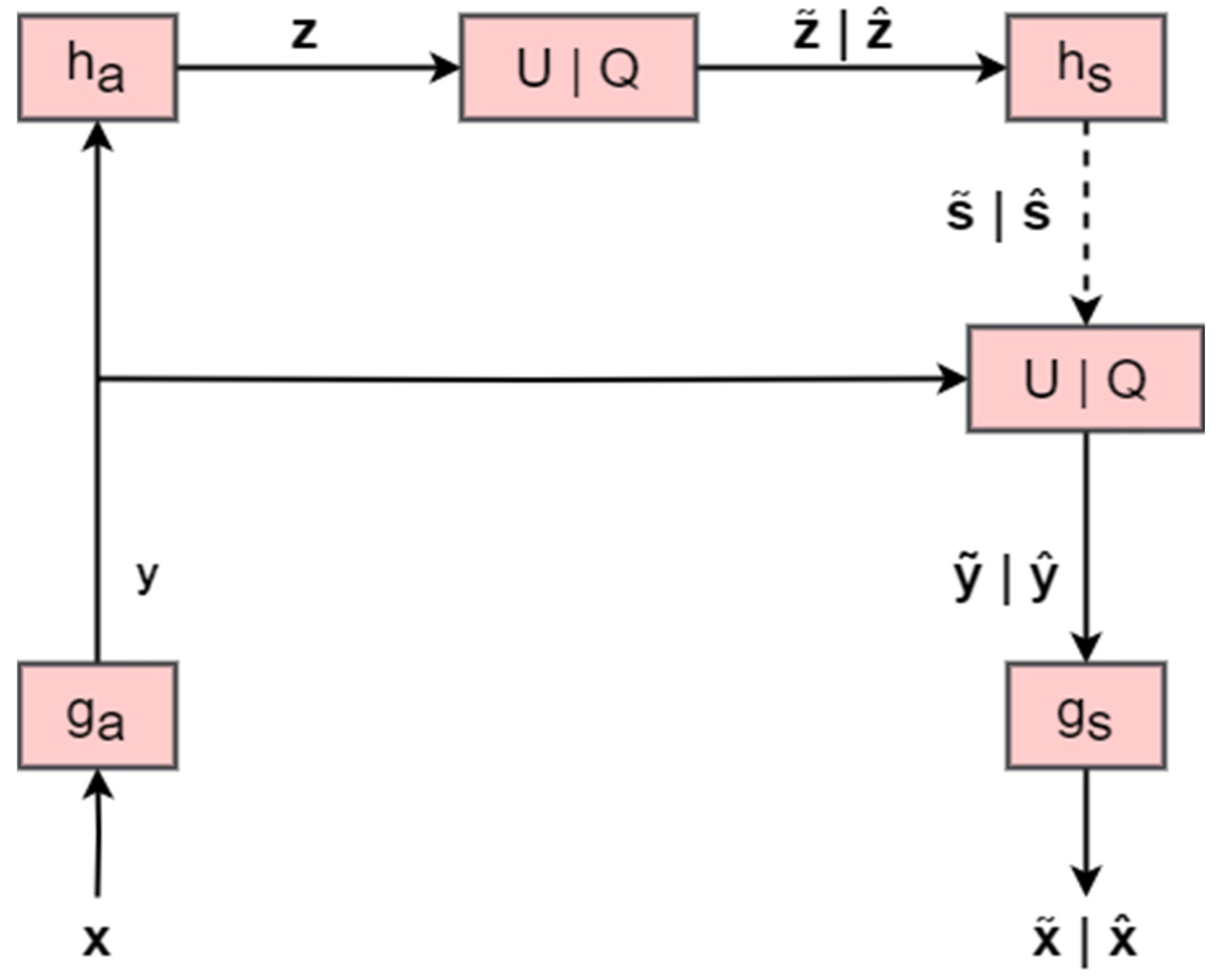
Figure 2 shows the operational diagram of the hyperprior model that serves as the foundation for the present technique. The input image x is fed to the base encoder ga, and the outputs y with spatially varying standard deviations are produced. These latents are then fed to the hyper encoder ha, summarizing the distribution of standard deviations in z, to which quantization or uniform noise addition and arithmetic encoding are applied afterwards. After this process, z ^ is used as side information by the hyper decoder hs for the estimation of the spatial distribution of standard deviations s ^ . The obtainment of s ^ combined with the responses y is used for the acquirement of y ^ as well. Finally, y ^ is fed to the base decoder gs, resulting in the reconstructed image x ^ . The synthesis transform is associated with the generative model, responsible for creating a reconstructed image from the latent representation, while the analysis transform is connected to the inference model, in charge of deducing the latent representation from the input image [31].
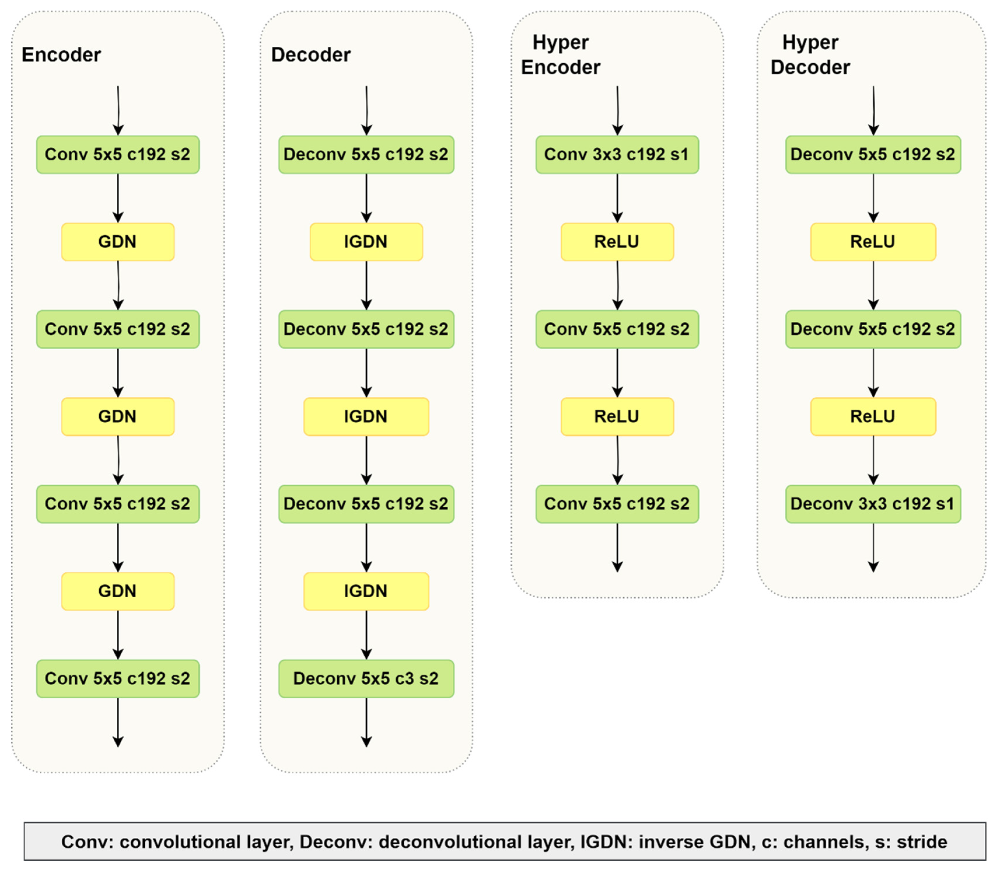
Our VAE network architecture closely resembles Ballé’s hyperprior architecture [31]. In an end-to-end approach, the common rectified linear unit function is replaced by a generalized divisive normalization (GDN) activation function [37], with each code assumed to follow a zero-mean Gaussian distribution, while the deviation is estimated by the side information network based on the hierarchical hyperprior. The bottlenecks of the base encoder, as well as that of the hyper encoder, go separately through quantization and entropy coding, before being combined again in the decoder. The VAE network is presented in Figure 3, while Figure 4 contains the individual network layers.
The final layer of the base encoder represents the code of the base autoencoder, with its output channels determining the number of features that need to be condensed and saved. Based on the trade-off between the rate and distortion, the proposed model learns to disregard specific channels by producing an identical latent value in a deterministic manner with a probability of 1, which, while computationally inefficient, needs no extra entropy. This method allows for setting a code that is larger than what is needed, giving the model the ability to determine the ideal number of channels for the best performance. It has been found that a too small number of channels in the code might hinder rate–distortion performance when training models for higher bit rates. However, a too big number of channels does not affect compression performance negatively [28]. We train our model for higher bit rates, so this is especially important. The higher bit rates are chosen because, after extensive experiments, we reached the conclusion that higher distortion metrics values have a positive impact on classification results. Finally, the last layer of the base decoder requires three channels in order to produce RGB images.
One substantial difference between our approach [26] and that of Ballé [31] is that we employ a different approach to represent the input images before feeding them to the network. Initially, we separate the images into their three color channels (red, green and blue). Then, as a preprocessing step, we apply the discrete wavelet transform (DWT) after the color channels are split. Each of the three resulting images undergoes discrete wavelet decomposition, resulting in four subimages corresponding to the approximation, horizontal, vertical, and diagonal details. Consequently, for each image taken from the original dataset, we obtain a total of 12 subimages. The post-processing step mirrors the pre-processing step. The proposed pre-processing operations are depicted in Figure 5.
The 3 subimages—one for each color channel— that represent the corresponding detail are combined to form a 3-channel image that is then fed to the corresponding neural network. This channel component stacking is different from our previous work [26] and is shown in Figure 6. The selected wavelet is the biorthogonal 4.4 wavelet, which is comparable to the 9/7 wavelet used in JPEG2000 and is regarded as well suited for lossy image compression [38].

3.2. Synthetic Image Detection

Most techniques rely on image features and distinctive attributes to distinguish between real and synthetic images, as has been described in Section 2. However, we have chosen to study image behavior after entropy-modelled compression. We utilize the quality metrics often seen in compression methods to decide the authenticity of an image. We take advantage of the fact that synthetic images in general fare better after being compressed and retain more of their original quality [39]. Furthermore, the quality of an image post-compression significantly affects the discernment of AI-generated images [40]. In addition, since we created 4 subimages for each initial one, we have more information available. While there are many ways of generating fake media, GAN-generated images are the most recent and the most common type of deepfakes [41,42,43], and we have focused our research on them. However, Diffusion Models have also been popular recently, and we are keen to explore these images too [44,45].
We found that the proposed learned compression technique worked differently on the subimages representing the four details of each image produced through the discrete wavelet transform. While approximation detail A loses a lot of its quality after the compression, diagonal detail D retains most of it. On the other hand, the horizontal and vertical details are somewhere in the middle. However, there is also a difference in the way natural and AI-generated images respond to the proposed model. Synthetic images appear to handle the compression better, resulting in better-quality reconstructed images both for the 4 subimages and for the final RGB image. The reconstruction quality gap between natural and artificial images is the biggest in the diagonal detail domain and the smallest for the final reconstructed image. We exploit these differentiations by compressing the images and utilizing the compression metrics for the discrimination of synthetic face images.
We use features of all four subimages as well as the final reconstructed image for the classification process. The loss and the bit rate (bpp) are the first factors considered. Additionally, the quality metrics have a significant impact, so MSE, MS-SSIM, peak signal-to-noise ratio (PSNR), and structural similarity (SSIM) are also taken into account. This leads to 6 features for each one of the 4 subimages. Additionally, the PSNR, SSIM, and MS-SSIM of the reconstructed image are also used, making a total of 27 features for each input image. However, every image is used by two models, A and B, so the number of extracted features doubles. In conclusion, 54 features are extracted from each image and used by a binary classifier. The features we use are illustrated in Figure 7.
The compression model is trained twice, once on a real and once on a synthetic dataset. For this reason, two identical models (Model A and Model B) are used. Model A is trained on real images and Model B is trained on fake ones. They need to be tested on both types of images, real and synthetic, since they work differently with these types of inputs. Thus, the testing datasets are split in half. The first half, real dataset 1 and synthetic dataset 1, are used for the evaluation of the two compression models. The features extracted from this process are given as inputs to the classifier for its training. The next step includes the same process for the two models with the other half of the testing dataset, only this time the output is used for the evaluation of the discriminator. This procedure is summarized in Process 1. After repeated experiments, we came to the conclusion that increasing the depth of the classifier does not improve the classification performance. Thus, an energy-efficient, not computationally complex option was chosen. The classifier is quite basic, and its layers are shown in Table 1.
Process 1. Discrimination of synthetic images
Step 1:Train compression model A on a real dataset
Train compression model B on a synthetic dataset
Step 2:Evaluate model A on real dataset 1
Evaluate model A on synthetic dataset 1
Evaluate model B on real dataset 1
Evaluate model B on synthetic dataset 1
Step 3:Train classifier on the features extracted from Step 2
Step 4:Evaluate model A on real dataset 2
Evaluate model A on synthetic dataset 2
Evaluate model B on real dataset 2
Evaluate model B on synthetic dataset 2
Step 5:Evaluate classifier on the features extracted from Step 4
Table 1. Classifier network layers.
Classifier
Dense 12
ReLU
Dense 8
ReLU
Dense 1
Sigmoid

4. Methodology and Experimental Results

In Section 4.1, we detail the datasets that were used for the experiments. A total of 4 datasets consisting of 38,000 images were used during our research. In Section 4.2, we explain the hyperparameters set for the training of our compression-based classification model. Finally, in Section 4.3, we discuss the performance of the present work and its robustness against image manipulations.

4.1. Datasets

A collection of 12,000 real face images was obtained from the CelebA_HQ dataset [46]. Of these, 10,000 images were used for training, constituting the real training dataset mentioned in Process 1, and 2000 images were used for testing. Half of these test images made up real dataset 1 and the other half made up real dataset 2. Several generative models were taken into account for the artificial face images, and we eventually decided to use the StyleGAN and StyleGAN2 datasets for our GAN-generated datasets. The StyleGAN subset [47] of synthetic images consists of 12,000 images in total; 10,000 images were used to train the model, comprising the synthetic training dataset, and 2000 images were used for testing. These testing images made up the synthetic datasets 1 and 2 mentioned in Process 1. We used the official release of the StyleGAN dataset and opted for a truncation parameter value of 0.5 to enhance the dataset’s variety. When the truncation parameter fades to 0, all faces converge to the “mean” face of FFHQ (the dataset which StyleGAN is trained on). This face is consistent across all trained networks, and interpolating towards it never appears to introduce artifacts. When applying higher scaling to styles, the result is the opposite, or “anti-face” [47]. The same logic is followed with the StyleGAN2 dataset [48]. We made these choices because StyleGAN and StyleGAN2 are trained on the FFHQ dataset [47], so there are no common aspects between the natural and artificial images. Additionally, we used an artificial dataset produced with stable diffusion for the testing in order to see whether the proposed method responds well to different kinds of synthetic images. This made up the final synthetic datasets 1 and 2 we used for testing in our experiments. We tested these datasets with models trained both on StyleGAN and on StyleGAN2. Table 2 presents a summary of the datasets utilized in our research.

4.2. Training Setting

All the images we used had a resolution of 1024 × 1024 pixels, and we cropped a square in the center of a size of 504 × 504 pixels. The same cropping was applied in both training and testing. The compression network could only handle images of a size larger than 256 × 256 pixels. This limitation combined with the dimensionality reduction caused by the DWT meant that the smallest image size we could use was 504 × 504 pixels. Resizing would be required for the classification of low-resolution images. However, resizing reduces the accuracy of the proposed model, so it inadvisable unless necessary. More details are given in Section 4.3.2. The cross-entropy loss function was used to train the network, along with the Adam optimizer [49]. Higher-quality images give better classification results, so we chose a value of 1000 for λ. The batch size was set to 8 and the learning rate had a steady value of 0.0001 for 250 epochs during training. Such a large number of epochs for the compression training was chosen since it is often beneficial to image compression methods [50,51]. On the other hand, the focus here was the discrimination of synthetic images, so 250 was a good compromise between the quality of the compressed image and the computational complexity. The binary classifier trained for 300 epochs with the batch size set to 16. While it is a simple network, it needs many epochs because of the number of features it takes as inputs. The Python3 environment and the Tensorflow library were used. The code is available on https://github.com/sof-il/SyntheticFaceDiscriminitor (accessed on 21 August 2024). Both the training and the testing of the model were implemented on an NVIDIA GeForce RTX 3080, 11 GB.

4.3. Results

4.3.1. Performance Analysis

In this analysis, we compare the suggested approach with one of the best available methods for identifying GAN-produced images. Gragnaniello et al. [21] reviewed multiple methods in their work. We focus on the variant of ResNet50 that involves the removal of downsampling from the first layer. This is a technique that is still used by many researchers to compare their results, since it works exceptionally well for GAN-generated images and is still unbeatable in some cases [15,25,52,53].
The metrics we used for the evaluation of our binary classifier were accuracy, precision, and recall (also known as True Positive Rate—TPR), as well as the area under the curve (AUC) of the receiver operating characteristic (ROC) curve. The first three metrics are defined in Equations (3)–(5), utilizing True Positives (TP), True Negatives (TN), False Positives (FP), and False Negatives (FN). Unlike accuracy, and like cross-entropy losses, AUC evaluates all the operational points of the model using a Riemann sum. The AUC is calculated using the height of the recall values with the False Positive Rate (FPR). This is defined in Equation (6). A linearly spaced set of 200 classification thresholds is used for the computation of TPR-FPR pairs [54]. The ROC curve illustrates the trade-off between these two metrics. The left side of the curve represents the more “confident” thresholds—a higher threshold results in lower recall and fewer False Positives. On the other hand, the right side of the curve corresponds to the “less strict” thresholds—a lower threshold increases both the recall and the False Positives. The ROC AUC is calculated by measuring the area under the ROC curve and has values from 0 to 1, though this is often changed to percentage form for ease. In Figure 8, we provide a graphical example of obtaining the ROC curve and the AUC from a chosen experiment.
a c c u r a c y = T P + T N T P + F P + T N + F N
p r e c i s i o n = T P T P + F P
r e c a l l = T P T P + F N
F P R = F P F P + T N
The initial experiments focus on evaluating the overall efficacy of the techniques being tested in discriminating synthetic face images. The results are given in Table 3 and Table 4.
The accuracy consistently remains above 95% regardless of the generation method of the dataset. As we can see in Table 3 and Table 4, we achieve better results with the StyleGAN dataset than StyleGAN2, for which our results are within 1% of those of ResNet50. Although for StyleGAN2 the accuracy of the detection is worse, it is still above 95%. The big difference between the results of the proposed method and ResNet50 comes when they are tested on images generated with stable diffusion. In this case, our compression-based method surpasses Resnet50 by far on all fronts. While Resnet50 achieves 49.70% accuracy, successfully detecting only real images, our technique does even better than with the GAN-generated datasets and reaches 99.00% and 99.10% accuracy. The precision and recall results are equally good, reaching almost 100%.

4.3.2. Robustness

We experimented with post-processing operations to see how well the proposed method fares against image manipulation and examine its robustness. The results are reported in Table 5 and Table 6. There are also visual representations of the exported data in Figure 9 and Figure 10.
The results clearly show that the proposed method is more effective for StyleGAN compared to StyleGAN2, but this does not hold true for the processed images. After post-processing, the second dataset seems to fare better on the deepfake detection front. This is interesting, given the fact that StyleGAN2 is more recent, and thus the generated face images are more realistic. We observe that our model is less impacted by Gaussian noise compared to ResNet50. The cropping also has no effect whatsoever, which was to be expected since we used a cropped version of the image anyway. The median filter affects our model more than ResNet50, with a 10% decline in StyleGAN accuracy. On the other hand, on StyleGAN2 it seems to work much better, with a less than 2% loss of accuracy. The proposed method also responds well to JPEG compression. However, the present work surpasses the performance of ResNet50 for the stable-diffusion-generated dataset for all types of “attacks”. Our technique maintains a stable performance of high accuracy, in most cases more than 90%. ResNet50, on the other hand, once again only detects real face images, failing in recognizing the diffusion-generated ones. In Figure 11, the performance of different JPEG quality factors is given. It is interesting that while for StyleGAN2 our method has a consistent performance, for StyleGAN it seems to improve as the quality factor increases.
As was stated above, the proposed method performs significantly better than ResNet50 when Gaussian noise is added to the images. This is caused by the nature of the “attack”. Gaussian noise affects the DWT of an image in several ways, primarily through the introduction of high-frequency components. It typically manifests as random variations in pixel values, predominantly affecting the high-frequency components of an image. During the DWT process, these high-frequency components are mapped to the detail coefficients. Consequently, the presence of Gaussian noise increases the magnitude of these detail coefficients. The diagonal detail that contains the high-frequency coefficients is extremely important to our method, as it displays the biggest variance between real and synthetic images. As a result, our compression-based technique performs much better than ResNet50 when faced with Gaussian noise. In order to prove this point even further, Figure 12 shows the behavior of both techniques when the images are “attacked” with Gaussian noise of different variances σ2, with the mean value being consistently zero.

5. Discussion

In this research, we performed thorough tests to assess the proposed method for the discrimination of synthetic face images. We used a deep learning-based image compression technique to detect synthetic face images. Additionally, we utilized the discrete wavelet transform to improve the detection process. This was established by noting that the diagonal details of a real and a synthetic face image display significant differences. On the other hand, the approximation details of real and synthetic faces are fairly similar, while the horizontal and vertical details have some differences, but not enough to be considered noteworthy. Instead of using image-specific features for this process, we compressed face images and measured the quality of their reconstruction, thus revealing their real or synthetic origin.
These experiments showed some interesting results. We proved that not only is it possible to use compression for deepfake detection, but the accuracy of such an attempt is comparable to that of GAN-based methods on GAN-generated faces. The robustness of the proposed technique was also tested against several image processing operations, proving beneficial against certain types of attacks, e.g., Gaussian noise. An important benefit of this approach is the reduced size of the neural networks needed for its implementation. While ResNet50—to which we compare our technique—is very efficient, it actually uses 49 layers. On the other hand, the proposed technique requires only 30 layers, 24 of which are used for the compression of the images and the other 6 for the classification. Consequently, there is lower computational complexity, which is highly beneficial. Finally, our method can successfully identify artificial images created using stable diffusion, in contrast to ResNet50, which seems to do well only on GAN-generated images. This means that the proposed method is more universal in regard to the images it can correctly classify.

6. Conclusions

In the present work, a novel solution to the problem of synthetic face discrimination is proposed. A learned image compression technique was used to detect synthetic images by evaluating compressed images’ quality. The research on this gives promising results, with accuracy close to 99% in many cases. A comparison to ResNet50 shows that our technique has accuracy results within 1% of this state-of-the-art method for images produced by GANs, and is far better for stable-diffusion-generated ones, while having lower complexity. We also experimented with some image processing operations to see how such “attacks” affect the model’s accuracy. Some of these operations proved to be ineffective against the proposed method, such as cropping, while others made the classification process more difficult. In conclusion, the use of compression for the discrimination of synthetic face images is a route that has not been explored yet. However, it has proven to be highly effective and deserves future study.

Author Contributions

Conceptualization, A.S.; methodology, S.I.; software, S.I. and P.T.; validation, A.S., D.A. and P.T.; formal analysis, S.I., A.S., D.A. and P.T.; investigation, S.I., D.A. and A.S.; resources, A.S.; data curation, S.I.; writing—original draft preparation, S.I.; writing—review and editing, A.S., D.A., and P.T.; visualization, A.S., D.A., P.T. and S.I.; supervision, A.S. and D.A.; project administration, A.S. All authors have read and agreed to the published version of the manuscript.

Funding

This research received no external funding.

Data Availability Statement

The data presented in this study are available on Github at https://github.com/sof-il/SyntheticFaceDiscriminitor; https://github.com/NVlabs/stylegan (accessed on 21 August 2024); https://github.com/NVlabs/stylegan2 (accessed on 21 August 2024); https://github.com/tkarras/progressive_growing_of_gans (accessed on 21 August 2024) and https://github.com/tobecwb/stable-diffusion-face-dataset (accessed on 21 August 2024) [40,41,42].

Conflicts of Interest

The authors declare no conflicts of interest.

References

  1. Dogoulis, P.; Kordopatis-Zilos, G.; Kompatsiaris, I.; Papadopoulos, S. Improving Synthetically Generated Image Detection in Cross-Concept Settings. In Proceedings of the 2nd ACM International Workshop on Multimedia AI against Disinformation (MAD ‘23), Thessaloniki, Greece, 12–15 June 2023; Association for Computing Machinery: New York, NY, USA, 2023; pp. 28–35. [Google Scholar] [CrossRef]
  2. Ramesh, A.; Dhariwal, P.; Nichol, A.; Chu, C.; Chen, M. Hierarchical text-conditional image generation with clip latents. arXiv 2022, arXiv:2204.06125. [Google Scholar]
  3. Goodfellow, I.; Pouget-Abadie, J.; Mirza, M.; Xu, B.; Warde-Farley, D.; Ozair, S.; Courville, A.; Bengio, Y. Generative Adversarial Networks. Commun. ACM 2020, 63, 139–144. [Google Scholar] [CrossRef]
  4. Karras, T.; Aittala, M.; Laine, S.; Härkönen, E.; Hellsten, J.; Lehtinen, J.; Aila, T. Alias-free generative adversarial networks. In Adv. Neural Inf. Process. Syst. 2021, 34, 852–863. [Google Scholar]
  5. Dhariwal, P.; Nichol, A. Diffusion models beat GANs on image synthesis. Adv. Neural Inf. Process. Syst. 2021, 34, 8780–8794. [Google Scholar]
  6. Rombach, R.; Blattmann, A.; Lorenz, D.; Esser, P.; Ommer, B. High-resolution image synthesis with latent diffusion models. In Proceedings of the IEEE/CVF Conference on Computer Vision and Pattern Recognition, New Orleans, LA, USA, 18–24 June 2022. [Google Scholar] [CrossRef]
  7. Farid, H. Photo Forensics; MIT Press: Cambridge, MA, USA, 2016. [Google Scholar]
  8. Guo, H.; Hu, S.; Wang, X.; Chang, M.C.; Lyu, S. Eyes Tell All: Irregular Pupil Shapes Reveal GAN-Generated Faces. In Proceedings of the 2022 IEEE International Conference on Acoustics, Speech and Signal Processing (ICASSP), Singapore, 23–27 May 2022; pp. 2904–2908. [Google Scholar] [CrossRef]
  9. Farid, H. Lighting (In)consistency of Paint by Text. arXiv 2022, arXiv:2207.13744. [Google Scholar]
  10. Farid, H. Perspective (In)consistency of Paint by Text. arXiv 2022, arXiv:2206.14617. [Google Scholar]
  11. Corvi, R.; Cozzolino, D.; Poggi, G.; Nagano, K.; Verdoliva, L. Intriguing Properties of Synthetic Images: From Generative Adversarial Networks to Diffusion Models. In Proceedings of the IEEE/CVF Conference on Computer Vision and Pattern Recognition (CVPR) Workshops, Vancouver, BC, Canada, 17–24 June 2023; pp. 973–982. [Google Scholar]
  12. Yang, X.; Li, Y.; Qi, H.; Lyu, S. Exposing GAN-synthesized Faces Using Landmark Locations. In Proceedings of the ACM Workshop on Information Hiding and Multimedia, Paris France, 3–5 July 2019; Association for Computing Machinery: New York, NY, USA, 2019; pp. 113–118. [Google Scholar] [CrossRef]
  13. Matern, F.; Riess, C.; Stamminger, M. Exploiting Visual Artifacts to Expose Deepfakes and Face Manipulations. In Proceedings of the 2019 IEEE Winter Applications of Computer Vision Workshops (WACVW), Waikoloa, HI, USA, 7–11 January 2019; pp. 83–92. [Google Scholar] [CrossRef]
  14. Nataraj, L.; Mohammed, T.M.; Manjunath, B.S.; Chandrasekaran, S.; Flenner, A.; Bappy, J.H.; Roy-Chowdhury, A. Detecting GAN generated Fake Images using Co-occurrence Matrices. Electron. Imaging 2019, 2019, 532-1–532-7. [Google Scholar] [CrossRef]
  15. Nowroozi, E.; Conti, M.; Mekdad, Y. Detecting High-Quality GAN-Generated Face Images using Neural Networks. arXiv 2022, arXiv:2203.01716. [Google Scholar]
  16. McCloskey, S.; Albright, M. Detecting GAN-Generated Imagery Using Saturation Cues. In Proceedings of the 2019 IEEE International Conference on Image Processing (ICIP), Taipei, Taiwan, 22–25 September 2019; pp. 4584–4588. [Google Scholar]
  17. Li, H.; Li, B.; Tan, S.; Huang, J. Identification of deep network generated images using disparities in color. Signal Process. 2020, 174, 107616. [Google Scholar] [CrossRef]
  18. Zhang, X.; Karaman, S.; Chang, S.-F. Detecting and Simulating Artifacts in GAN Fake Images. In Proceedings of the 2019 IEEE International Workshop on Information Forensics and Security (WIFS), Delft, The Netherlands, 9–12 December 2019; pp. 1–6. [Google Scholar] [CrossRef]
  19. Frank, J.; Eisenhofer, T.; Schönherr, L.; Fischer, A.; Kolossa, D.; Holz, T. Leveraging frequency analysis for deep fake image recognition. arXiv 2020, arXiv:2003.08685. [Google Scholar]
  20. Durall, R.; Keuper, M.; Keuper, J. Watch Your Up-Convolution: CNN Based Generative Deep Neural Networks Are Failing to Reproduce Spectral Distributions. In Proceedings of the 2020 IEEE/CVF Conference on Computer Vision and Pattern Recognition (CVPR), Seattle, WA, USA, 13–19 June 2020; pp. 7887–7896. [Google Scholar] [CrossRef]
  21. Gragnaniello, D.; Cozzolino, D.; Marra, F.; Poggi, G.; Verdoliva, L. Are GAN Generated Images Easy to Detect? A Critical Analysis of the State-Of-The-Art. In In Proceedings of the 2021 IEEE International Conference on Multimedia and Expo (ICME), Shenzhen, China, 5–9 July 2021; pp. 1–6. [Google Scholar] [CrossRef]
  22. Boroumand, M.; Chen, M.; Fridrich, J. Deep Residual Network for Steganalysis of Digital Images. IEEE Trans. Inf. Forensics Secur. 2019, 14, 1181–1193. [Google Scholar] [CrossRef]
  23. Wang, J.; Tondi, B.; Barni, M. An Eyes-Based Siamese Neural Network for the Detection of GAN-Generated Face Images. Front. Signal Process. 2022, 2, 918725. [Google Scholar] [CrossRef]
  24. Fu, T.; Xia, M.; Yang, G. Detecting GAN-generated face images via hybrid texture and sensor noise-based features. Multimed. Tools Appl. 2022, 81, 26345–26359. [Google Scholar] [CrossRef]
  25. Cozzolino, D.; Poggi, G.; Corvi, R.; Nießner, M.; Verdoliva, L. Raising the Bar of AI-generated Image Detection with CLIP. arXiv 2023, arXiv:2312.00195. [Google Scholar] [CrossRef]
  26. Iliopoulou, S.; Tsinganos, P.; Ampeliotis, D.; Skodras, A. Learned Image Compression with Wavelet Preprocessing for Low Bit Rates. In Proceedings of the 2023 24th International Conference on Digital Signal Processing (DSP), Rhodes, Greece, 11–13 June 2023; pp. 1–5. [Google Scholar] [CrossRef]
  27. Li, M.; Zhang, K.; Li, J.; Zuo, W.; Timofte, R.; Zhang, D. Learning Context-Based Nonlocal Entropy Modeling for Image Compression. IEEE Trans. Neural Netw. Learn. Syst. 2023, 34, 1132–1145. [Google Scholar] [CrossRef] [PubMed]
  28. Minnen, D.; Ballé, J.; Toderici, G.D. Joint Autoregressive and Hierarchical Priors for Learned Image Compression. Adv. Neural Inf. Process. Syst. 2018, 31, 10771–10780. [Google Scholar]
  29. Cover, T.M.; Thomas, J.A. Data Compression. In Elements of Information Theory, 2nd ed.; John Wiley & Sons: Hoboken, NJ, USA, 2021; pp. 103–142. [Google Scholar]
  30. Toderici, G.; Vincent, D.; Johnston, N.; Hwang, S.; Minnen, D.; Shor, J.; Covell, M. “Full resolution image compression with recurrent neural networks. In Proceedings of the 2017 IEEE Conference on Computer Vision Pattern Recognit. (CVPR), Honolulu, HI, USA, 21–26 July 2017; pp. 5435–5443. [Google Scholar]
  31. Balle, J.; Minnen, D.; Singh, S.; Hwang, S.J.; Johnston, N. Variational image compression with a scale hyperprior. In Proceedings of the 6th International Conference on Learning Representations, Vancouver, BC, Canada, 30 April–3 May 2018. [Google Scholar]
  32. Ballé, J.; Laparra, V.; Simoncelli, E.P. End-to-end optimized image compression. In Proceedings of the 5th International Conference on Learning Representations, Toulon, France, 24–26 April 2017. [Google Scholar]
  33. Qian, Y.; Tan, Z.; Sun, X.; Lin, M.; Li, D.; Sun, Z.; Li, H.; Jin, R. Learning accurate entropy model with global reference for image compression. In Proceedings of the International Conference on Learning Representations (ICLR), Virtual Event, Austria, 3–7 May 2021. [Google Scholar]
  34. Wang, Z.; Simoncelli, E.P.; Bovik, A.C. Multiscale structural similarity for image quality assessment. In Proceedings of the 37th Asilomar Conference on Signals, Systems & Computers, Pacific Grove, CA, USA, 9–12 November 2003; Volume 2, pp. 1398–1402. [Google Scholar] [CrossRef]
  35. Theis, L.; Shi, W.; Cunningham, A.; Huszár, F. Lossy Image Compression with Compressive Autoencoders. arXiv 2017, arXiv:1703.00395. [Google Scholar]
  36. Ballé, J.; Laparra, V.; Simoncelli, E.P. End-to-end optimization of nonlinear transform codes for perceptual quality. In Proceedings of the 2016 Picture Coding Symposium (PCS), Nuremberg, Germany, 4–7 December 2016; pp. 1–5. [Google Scholar] [CrossRef]
  37. Ballé, J.; Laparra, V.; Simoncelli, E.P. Density Modeling of Images using a Generalized Normalization Transformation. In Proceedings of the 4th International Conference on Learning Representations, ICLR 2016, San Juan, Puerto Rico, 2–4 May 2016. Conference Track Proceedings 2016. [Google Scholar]
  38. Skodras, A.; Christopoulos, C.; Ebrahimi, T. The JPEG 2000 still image compression standard. IEEE Signal Process. Mag. 2001, 18, 36–58. [Google Scholar] [CrossRef]
  39. Bruckstein, A.M.; Elad, M.; Kimmel, R. Down-scaling for better transform compression. IEEE Trans. Image Process. 2003, 12, 1132–1144. [Google Scholar] [CrossRef]
  40. Chen, P.; Xu, M.; Wang, X. Detecting Compressed Deepfake Images Using Two-Branch Convolutional Networks with Similarity and Classifier. Symmetry 2022, 14, 2691. [Google Scholar] [CrossRef]
  41. Liu, C.; Zhu, T.; Shen, S.; Zhou, W. Towards Robust Gan-Generated Image Detection: A Multi-View Completion Representation. In Proceedings of the 32nd International Joint Conference on Artificial Intelligence (IJCAI-23), Macau SAR, China, 19–25 August 2023; pp. 464–472. [Google Scholar] [CrossRef]
  42. Marra, F.; Gragnaniello, D.; Cozzolino, D.; Verdoliva, L. Detection of GAN-Generated Fake Images Over Social Networks. In Proceedings of the 2018 IEEE Conference on Multimedia Information Processing and Retrieval (MIPR), Miami, FL, USA, 10–12 April 2018; pp. 384–389. [Google Scholar] [CrossRef]
  43. Dong, C.; Kumar, A.; Liu, E. Think Twice Before Detecting GAN-generated Fake Images from their Spectral Domain Imprints. In Proceedings of the 2022 IEEE/CVF Conference on Computer Vision and Pattern Recognition (CVPR), New Orleans, LA, USA, 18–24 June 2022; pp. 7855–7864. [Google Scholar] [CrossRef]
  44. Stockl, A. Evaluating a Synthetic Image Dataset Generated with Stable Diffusion. In Proceedings of the Eighth International Congress on Information and Communication Technology, London, UK, 20–23 January 2023; pp. 805–818. [Google Scholar]
  45. Corvi, R.; Cozzolino, D.; Zingarini, G.; Poggi, G.; Nagano, K.; Verdoliva, L. On the Detection of Synthetic Images Generated by Diffusion Models. In Proceedings of the 2023 IEEE International Conference on Acoustics, Speech and Signal Processing (ICASSP), Rhodes, Greece, 4–10 June 2023; pp. 1–5. [Google Scholar] [CrossRef]
  46. Karras, T.; Aila, T.; Laine, S.; Lehtinen, J. Progressive Growing of GANs for Improved Quality, Stability, and Variation. In Proceedings of the International Conference on Learning Representations, Toulon, France, 24–26 April 2017. [Google Scholar]
  47. Karras, T.; Laine, S.; Aila, T. A Style-Based Generator Architecture for Generative Adversarial Networks. IEEE Trans. Pattern Anal. Mach. Intell. 2021, 43, 4217–4228. [Google Scholar] [CrossRef]
  48. Karras, T.; Laine, S.; Aittala, M.; Hellsten, J.; Lehtinen, J.; Aila, T. Analyzing and Improving the Image Quality of StyleGAN. In Proceedings of the IEEE/CVF Conference on Computer Vision and Pattern Recognition, Seattle, WA, USA, 13–19 June 2020. [Google Scholar]
  49. Kingma, D.P.; Ba, J. Adam: A Method for Stochastic Optimization. arXiv 2014, arXiv:1412.6980,. [Google Scholar]
  50. Perugachi-Diaz, Y.; Gansekoele, A.; Bhulai, S. Robustly overfitting latents for flexible neural image compression. arXiv 2024, arXiv:2401.17789. [Google Scholar]
  51. Mikami, Y.; Tsutake, C.; Takahashi, K.; Fujii, T. An Efficient Image Compression Method Based on Neural Network: An Overfitting Approach. In Proceedings of the 2021 IEEE International Conference on Image Processing (ICIP), Anchorage, AK, USA, 19–22 September 2021; pp. 2084–2088. [Google Scholar] [CrossRef]
  52. Wu, H.; Zhou, J.; Zhang, S. Generalizable Synthetic Image Detection via Language-guided Contrastive Learning. arXiv 2023, arXiv:2305.13800. [Google Scholar]
  53. Wang, J.; Alamayreh, O.; Tondi, B.; Barni, M. Open Set Classification of GAN-based Image Manipulations via a ViT-based Hybrid Architecture. In Proceedings of the 2023 IEEE/CVF Conference on Computer Vision and Pattern Recognition Workshops (CVPRW), Vancouver, BC, Canada, 20–22 June 2023; pp. 953–962. [Google Scholar] [CrossRef]
  54. Classification Metrics Based on True/False Positives & Negatives. Keras. Available online: https://keras.io/api/metrics/classification_metrics/ (accessed on 1 August 2024).
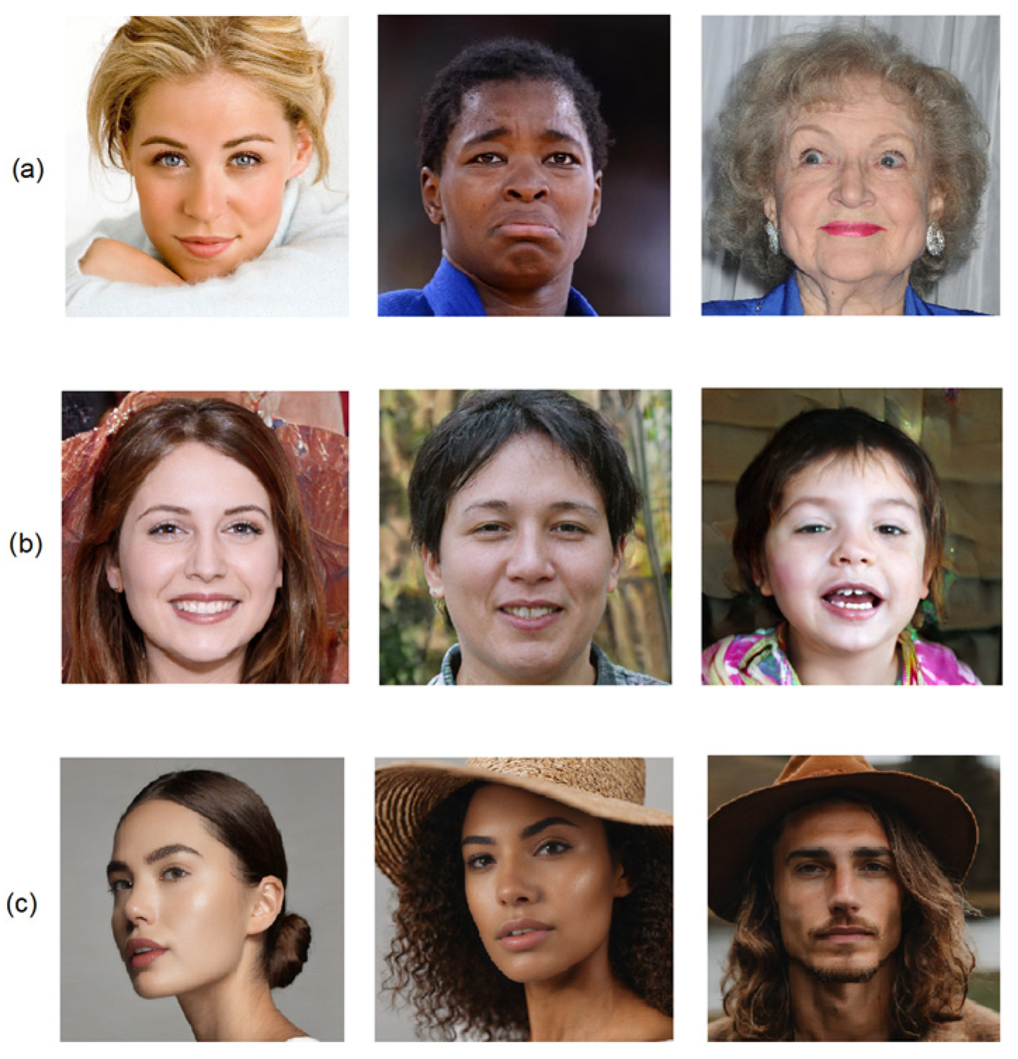
Figure 1. Natural and synthetic images of human faces. (a) Natural faces from the CelebA_HQ dataset, (b) synthetic faces from the StyleGAN2 dataset, and (c) synthetic faces produced with stable diffusion.
Algorithms 17 00375 g001
Figure 2. Operational diagram of the hyperprior model. The squares indicate transformations of the data and the arrows represent the direction of data flow. The boxes U|Q represent either the addition of uniform noise in the training phase (generating the vectors with a tilde) or quantization and arithmetic coding in the testing phase (generating the vectors with a hat).
Algorithms 17 00375 g002
Figure 3. The architecture of the VAE network. Q represents quantization, AE stands for the (lossless) arithmetic encoder, and AD is the arithmetic decoder.
Algorithms 17 00375 g003
Figure 4. Compression network layers.
Algorithms 17 00375 g004
Figure 5. The pre-processing stage, consisting of channel splitting, normalization, DWT, and channel stacking.
Algorithms 17 00375 g005
Figure 6. Channel component stacking.
Algorithms 17 00375 g006
Figure 7. Features used for the discrimination of synthetic images. For each image, 27 features are extracted from the model trained on real images and 27 are extracted from the model trained on AI-generated images.
Algorithms 17 00375 g007
Figure 8. The ROC curve represents the performance of our binary classifier on a StyleGAN synthetic image after the application of a 3 × 3 median filter at different classification thresholds. The default threshold is 0.5, but to obtain the ROC curve we use values from 0 to 1. The calculation of the AUC metric requires the measurement of the area under the ROC curve (0.961).
Algorithms 17 00375 g008
Figure 9. Accuracy, AUC, precision, and recall results comparison.
Algorithms 17 00375 g009
Figure 10. Accuracy, AUC, precision, and recall results comparison for “attacked” images resized by a factor of 0.5.
Algorithms 17 00375 g010
Figure 11. Accuracy of the proposed technique and ResNet50 when JPEG compression with various quality factors is applied to the image.
Algorithms 17 00375 g011
Figure 12. Accuracy of the proposed method and ResNet50 when Gaussian noise of different variance values is applied to the image.
Algorithms 17 00375 g012
Table 2. Face datasets used for training and testing.
DatasetsCelebA_HQStyleGANStyleGAN2Stable Diffusion
ClassRealSyntheticSyntheticSynthetic
Training10,00010,00010,000None
Testing2000200020002000
Table 3. Accuracy (ACC) and AUC results.
DatasetACC/AUC
Our MethodResNet50
StyleGAN98.90/100.099.70/100.0
StyleGAN295.30/99.099.70/100.0
Stable Diffusion (our model trained on StyleGAN)99.00/100.049.70/32.50
Stable Diffusion (our model trained on StyleGAN2)99.10/99.9049.70/32.50
Bold entries indicate the best results for each scenario.
Table 4. Precision and recall results.
DatasetPrecision/Recall
Our MethodResNet50
StyleGAN98.60/99.20100.0/99.40
StyleGAN295.20/95.40100.0/99.40
Stable Diffusion (our model trained on StyleGAN)99.20/99.5049.84/99.40
Stable Diffusion (our model trained on StyleGAN2)98.81/99.4049.84/99.40
Bold entries indicate the best results for each scenario.
Table 5. Accuracy (ACC) and AUC results for “attacked” images under various image processing operations.
Processing OperationACC/AUC
StyleGANStyleGAN2Stable Diffusion (Our Model Trained on StyleGAN)Stable Diffusion (Our Model Trained on StyleGAN2)
Our MethodResNet50Our MethodResNet50Our MethodResNet50Our MethodResNet50
Gaussian noise (σ2 = 0.01)97.90/99.3064.60/58.3095.30/98.9064.60/64.8098.30/99.5049.90/54.2097.70/99.8049.90/54.20
Median filter (3 × 3)88.20/97.3099.90/99.9093.50/97.9099.80/99.9095.30/99.1049.90/51.1096.40/98.9049.90/51.10
JPEG (QF = 90)94.00/97.1099.70/99.8095.30/98.8099.70/99.8098.60/99.9049.70/42.6098.30/99.8049.70/42.60
Cropping (512 × 512)98.90/100.099.30/98.7095.30/99.099.20/98.7099.00/100.049.30/39.5099.10/99.9049.30/39.50
Resize (0.5)98.40/99.60100.0/99.9094.40/98.8088.60/91.3098.50/99.8050.00/50.8099.20/99.9050.00/50.80
Resize (1.5)94.10/98.20100.0/100.092.30/98.10100.0/100.094.70/98.6050.00/50.4093.90/98.9050.00/50.40
Bold entries indicate the best results for each scenario.
Table 6. Precision and recall results for “attacked” images under various image processing operations.
Processing OperationPrecision/Recall
StyleGANStyleGAN2Stable Diffusion (Our Model Trained on StyleGAN)Stable Diffusion (Our Model Trained on StyleGAN2_
Our MethodResNet50Our MethodResNet50Our MethodResNet50Our MethodResNet50
Gaussian noise (σ2 = 0.01)97.60/98.20100.0/29.2094.50/96.20100.0/29.2098.99/97.6049.95/99.8099.18/96.2049.95/99.80
Median filter (3 × 3)96.40/79.40100.0/99.8091.90/95.40100.0/99.8095.21/95.4049.95/99.8095.14/97.8049.95/99.80
JPEG (QF = 90)92.64/95.60100.0/99.4094.50/96.20100.0/99.4098.80/98.4049.84/99.4098.20/98.4049.84/99.40
Cropping (512 × 512)98.60/99.20100.0/98.6095.20/95.40100.0/98.6099.20/99.5049.65/98.6098.81/99.4049.30/98.60
Resize (0.5)98.99/97.80100.0/100.092.05/97.2081.43/100.098.50/99.8050.00/100.0099.20/99.9050.00/100.00
Resize (1.5)93.00/97.40100.0/100.092.50/93.20100.0/100.094.60/94.8050.00/100.0093.10/93.6050.00/100.00
Bold entries indicate the best results for each scenario.
Disclaimer/Publisher’s Note: The statements, opinions and data contained in all publications are solely those of the individual author(s) and contributor(s) and not of MDPI and/or the editor(s). MDPI and/or the editor(s) disclaim responsibility for any injury to people or property resulting from any ideas, methods, instructions or products referred to in the content.