Abstract
Traffic prediction is crucial for transportation management and user convenience. With the rapid development of deep learning techniques, numerous models have emerged for traffic prediction. Recurrent Neural Networks (RNNs) are extensively utilized as representative predictive models in this domain. This paper comprehensively reviews RNN applications in traffic prediction, focusing on their significance and challenges. The review begins by discussing the evolution of traffic prediction methods and summarizing state-of-the-art techniques. It then delves into the unique characteristics of traffic data, outlines common forms of input representations in traffic prediction, and generalizes an abstract description of traffic prediction problems. Then, the paper systematically categorizes models based on RNN structures designed for traffic prediction. Moreover, it provides a comprehensive overview of seven sub-categories of applications of deep learning models based on RNN in traffic prediction. Finally, the review compares RNNs with other state-of-the-art methods and highlights the challenges RNNs face in traffic prediction. This review is expected to offer significant reference value for comprehensively understanding the various applications of RNNs and common state-of-the-art models in traffic prediction. By discussing the strengths and weaknesses of these models and proposing strategies to address the challenges faced by RNNs, it aims to provide scholars with insights for designing better traffic prediction models.
1. Introduction
Traffic prediction plays a crucial role in intelligent urban management and planning research on traffic prediction, encompassing various aspects such as traffic flow on road networks, passenger flow on public transit networks, Origin–Destination (OD) demand prediction, traffic speed prediction, travel time prediction, traffic congestion prediction, etc., holds significant importance for both users and managers of transportation systems. Accurate traffic prediction enables users to plan their routes more effectively, whether driving on roads or using public transit. By avoiding congested areas and selecting the most efficient paths, users can reduce travel time and improve their overall commuting experience. Additionally, predicting traffic conditions allows users to anticipate potential hazards, accidents, or delays along their route, enabling them to make safer decisions while navigating roads or utilizing public transportation services. Moreover, real-time access to traffic predictions empowers users to make informed decisions about when to travel, which routes to take, or whether to switch to alternative modes of transportation. This leads to increased convenience and flexibility in managing their daily commutes. For urban planners and traffic managers, traffic prediction research assists transportation managers in optimizing the performance of road and transit networks by identifying congestion-prone areas and implementing appropriate traffic management strategies. This includes adjusting traffic signal timings, optimizing public transit schedules, and coordinating infrastructure improvements to enhance network efficiency. Additionally, accurate traffic predictions enable managers to allocate resources more effectively, such as deploying additional transit services, adjusting route schedules, or prioritizing maintenance activities. This ensures that resources are utilized efficiently to meet the demands of travelers and minimize disruptions. Moreover, insights derived from traffic prediction research inform strategic decision-making processes related to urban planning, infrastructure development, and transportation policy formulation. By understanding future traffic patterns and demands, decision makers can make informed choices to support sustainable and resilient transportation systems. In summary, research on traffic prediction plays a critical role in optimizing travel efficiency, safety, and convenience for users while assisting transportation managers in effectively managing and improving the performance of transportation networks.
Traditional traffic prediction methods, such as those based on Historical Averages (HAs), time series analysis, and autoregressive models, while providing initial traffic prediction to some extent, often fail to fully capture traffic data’s complexity and dynamic changes. These methods typically assume that traffic variations are linear or follow simple patterns, making it challenging to handle non-linear relationships, the impact of sudden events, and seasonal or periodic changes in traffic data. Additionally, they exhibit low efficiency when dealing with large-scale, high-dimensional data, making it challenging to respond to real-time traffic changes. In recent years, the rapid development of deep learning models has dramatically promoted research and applications in traffic prediction. Deep learning models such as Recurrent Neural Networks (RNNs), Convolutional Neural Networks (CNNs), Graph Neural Networks (GNNs), and transformers have provided new solutions for traffic prediction with their outstanding data processing capabilities and ability to model complex temporal and spatial relationships. These models can automatically learn traffic flow patterns, passenger flow, speed, and congestion changes from massive historical traffic data, achieving high-accuracy predictions of future traffic conditions.
Given the impact of deep learning on traffic prediction, the significance of RNNs and their variants, such as long short-term memory (LSTM) networks and Gated Recurrent Unit (GRU) networks, stands out prominently. The design philosophy of RNNs enables them to naturally handle time series data, which is crucial for traffic prediction as traffic features, like flow and speed, vary over time. By capturing long-term dependencies in time series, RNNs can accurately forecast future changes in traffic conditions. Mainly, variants of RNNs, like LSTMs and GRUs, address the issue of vanishing or exploding gradients faced by traditional RNNs when dealing with long sequences through specialized gating mechanisms. This further enhances prediction accuracy and stability.
As neural network models for traffic prediction become increasingly popular, the diversification of deep learning models complicates the assessment of the current state and future directions of this research field. Despite the emergence of advanced models, like transformers, which have demonstrated superior performance in traffic prediction, reviewing the applications of RNNs in this field remains essential. Recent developments, such as the introduction of the Test-Time Training (TTT) [1] and the Extend LSTM (xLSTM) model by the original author of LSTM in 2024 [2], have reinvigorated interest in RNNs, showcasing their exceptional predictive capabilities and highlighting a resurgence in their relevance. RNNs offer a critical baseline for evaluating newer architectures, and understanding RNNs’ capabilities and limitations provides valuable insights into model design and optimization, which can still be advantageous in specific contexts.
The scarcity of specialized studies on RNN models further complicates understanding their application in traffic prediction. This review addresses these challenges by providing a comprehensive overview, targeting professionals interested in applying RNNs for traffic prediction. Starting with the definition of the problem and a brief history of traffic prediction, it then delves into RNNs within traffic prediction research. It discusses the comparison between RNNs and other state-of-the-art methods and the challenges RNNs face in traffic prediction.
The insights that can be extracted from this paper are as follows:
- The unique characteristics of traffic data and common input data representations in traffic prediction are summarized.
- The statement of traffic prediction problems is generalized.
- A comprehensive overview of seven sub-categories of applications of current deep learning models based on the structures of RNNs in traffic prediction is conducted.
- A detailed comparison between RNNs and other state-of-the-art deep learning models is conducted. In addition to the comparison of RNNs with other state-of-the-art models on public datasets, such as the Performance Measurement System (PeMS, http://pems.dot.ca.gov/ (accessed on 2 March 2024)), we design a comparative study focused on short-term passenger flow prediction using a real-world metro smart card dataset. This study allows us to directly compare the predictive performance of RNNs with other models in a practical, real-world context.
- Transformers excel with long sequences and complex patterns, but RNNs can outperform with shorter sequences and smaller datasets. The metro data used in our comparative study favored LSTM, showing that simpler models can sometimes provide more accurate and efficient predictions. Choosing the right model based on the dataset and resources is crucial.
- The future challenges facing RNNs in traffic prediction and how to deal with these challenges are discussed.
The paper is structured as follows.
In Section 2, we review the development history of the traffic prediction field over the past six decades and describe various data-driven prediction methods. We categorize prediction methods into three major classes: statistical methods, traditional machine learning, and deep learning. With the enhancement of computational resources and advancement in data acquisition techniques, deep learning has gradually become mainstream due to its outstanding performance in prediction accuracy.
In Section 3, we introduce traffic data and its unique characteristics, summarize the abstract description of traffic prediction problems, and then discuss the impact of input data representation on RNNs and their variants for traffic prediction. This includes the form of input sequences (including time series, matrix/grid-based sequences, and graph-based sequences) and sliding window techniques. This section emphasizes the importance of accurately representing input data to improve the prediction accuracy of RNN models. It discusses the performance differences when handling different data representations, ranging from simple RNNs to complex models combining CNNs and GNNs.
In Section 4, we delve into RNNs and their variants, sequentially introducing classical methods and hybrid models (such as RNNs combined with machine learning techniques, CNNs, GNNs, and attention mechanisms). This section showcases RNNs’ advantages in capturing temporal dependencies and methods for overcoming limitations and enhancing prediction performance through integration with other technologies.
In Section 5, we delve into the application of RNNs and their variants in traffic prediction, covering seven aspects as follows: traffic flow prediction, passenger flow prediction, OD (Origin–Destination) demand prediction, traffic speed prediction, travel time prediction, traffic accidents and congestion prediction, and occupancy prediction. This section provides a detailed exposition of the performance of relevant models in various domains.
In Section 6, we discuss the comparison between RNNs and the most popular models, i.e., transformer series models, as well as other classical prediction models, such as convolutional-based time series prediction models. This section also explores the challenges faced, such as model interpretability, accuracy in long-term prediction, the lack of standardized benchmark datasets, issues with small sample sizes and missing data, and the challenge of integrating heterogeneous data from multiple sources.
2. Development History of Traffic Prediction
In this section, we conduct a thorough review and survey of significant research on traffic prediction throughout its development history. The field of traffic prediction has evolved over nearly six decades, during which various prediction methods have emerged. Traffic prediction is a multidimensional research field encompassing a diverse classification of methods and applications (Figure 1). Methodologically, traffic prediction is divided into three major classes: statistical methods, traditional machine learning methods, and deep learning methods. Moreover, traffic prediction involves multiple sub-areas of applications, such as traffic flow prediction, passenger flow prediction, traffic speed prediction, and travel time prediction. These sub-areas will be explored in detail in Section 5. This section will systematically review traffic prediction’s historical development and technological progress, following the aforementioned methodological classification. Statistical methods are particularly suitable for handling smaller datasets due to their clear and simplified computational frameworks compared to more advanced machine learning techniques. Meanwhile, traditional machine learning methods excel in capturing complex non-linear relationships in traffic data and processing high-dimensional data. With the enhancement of computational power and improvement in data acquisition methods, deep learning methods are increasingly popular due to their complex structures and ability to outperform many traditional methods given sufficient data.
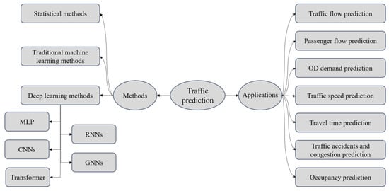
Figure 1.
A taxonomy of traffic prediction methods and applications.
2.1. Statistical Methods
Statistical methods play pivotal roles in traffic prediction, representing a major paradigm of data-driven methodologies. Statistical methods, exemplified by time series analysis encompassing HA models [3], Exponential Smoothing models (ES) [4], ARIMA models [5], Vector Auto Regression (VAR) models [6], etc., rely on the statistical attributes of historical data to anticipate forthcoming traffic. By capturing the temporal dependencies and seasonal patterns inherent in traffic data, these methodologies furnish a robust groundwork for short-term and mid-term traffic forecasting.
In time series analysis, the ARIMA model and its variants represent mature methodologies rooted in classical statistics and have been widely applied in traffic prediction tasks [7,8,9,10,11]. Ahmed et al. [12] were the first to use the ARIMA model for traffic prediction problems. Since then, many scholars have made improvements in this area. For example, Williams et al. [13] proposed seasonal ARIMA to predict traffic flow, considering the periodicity of traffic data. The success of these models lies in their ability to capture trends and seasonal patterns in time series data, thereby providing accurate predictions for domains, such as traffic volume and accident rates. However, despite the efficacy of the ARIMA model and its variants in addressing linear time series forecasting problems, they exhibit certain limitations, mainly when dealing with complex issues, like traffic prediction. Firstly, ARIMA models assume data has linear relationships and fail to capture non-linear patterns in traffic flow data. Secondly, ARIMA models are limited to a small set of features (lags of the time series itself) and struggle to integrate external factors affecting traffic, such as weather. Additionally, these models are computationally unsuitable for handling large or high-dimensional datasets and require manual tuning of parameters. ARIMA models are sensitive to missing data and noise, necessitating preprocessing and imputation to address gaps in the time series. Their capability for real-time prediction is limited, especially when the models need frequent retraining.
2.2. Traditional Machine Learning Methods
Traditional machine learning methods in traffic prediction practice mainly fall into three categories: feature-based models, Gaussian process models, and state space models. Feature-based models, particularly suitable for traffic prediction [14], rely on regression models constructed from statistical and traffic features. The challenge with such methods lies in the manual construction of regression models, with their effectiveness largely dependent on the accuracy of regression analysis. Zheng et al. [15] proposed a feature selection-based method to explore the performance of machine learning models, such as Support Vector Regression (SVR) and K-Nearest Neighbor (K-NN), in predicting traffic speed across various feature selections. On the other hand, Gaussian process models involve complex manipulation of the spatiotemporal attributes of traffic data. While accurate, scaling to large datasets is difficult due to its high computational resource requirements [16,17]. Sun et al. [18] proposed a method for a mixture of variational approximate Gaussian processes, which extends the single Gaussian process regression model. Zhao et al. [19] established a fourth-order Gaussian process dynamical model for traffic flow prediction based on K-NN, achieving significant improvements. State space models operate by simulating the uncertainty of the system through Markovian hidden states. While they demonstrate specific capabilities in simulating complex systems and dynamic traffic flows, their application is limited when dealing with more intricate traffic simulations and flow dynamics [20]. Shin et al. [21] utilized a Markov chain with velocity constraints to stochastically generate velocity trajectories for traffic speed prediction. Zhu et al. [22] chose the hidden Markov model to represent the dynamic transition process of traffic states and used it to estimate traffic states.
2.3. Deep Learning Methods
While traditional machine learning models can effectively learn non-linear patterns in data, they still have limitations, such as requiring extensive feature engineering, struggling with high-dimensional data, and not capturing complex temporal dependencies as effectively. With their multi-layer neural network structures, deep learning models provide a powerful capability for handling such data. Due to their numerous layers and large number of parameters, these models are particularly suitable for extracting features from large and complex datasets, thereby achieving excellent predictive performance. This leads to the success of deep learning in multiple fields, such as stock prediction [23], text mining [24], and traffic prediction.
Deep learning provides a powerful tool for handling high-dimensional data and learning complex patterns, with Multi-Layer Perceptron (MLP) [25] being one of the most basic deep learning networks that has shown significant potential in traffic prediction. MLP is a feedforward neural network consisting of an input layer, several hidden layers, and an output layer. It is suitable for performing classification and regression tasks, which are crucial in traffic prediction. The goals of traffic prediction include but are not limited to predicting traffic flow, vehicle speed, travel time, and congestion levels. MLPs use backpropagation as a training technique, a supervised learning algorithm that learns the desired output from diverse inputs. Early research applying MLPs to traffic prediction was mainly performed around 1995. For example, Taylor et al. [26] applied MLPs to predict highway traffic volume and occupancy, while Ledoux [27] summarized the potential applications of MLPs in traffic flow modeling. Despite MLP’s early widespread application in traffic prediction due to its ability to handle non-linear relationships in traffic data, more powerful and specifically optimized deep learning models are gradually replacing MLPs over time.
The subsequent development of RNNs represents a significant evolution of traditional feedforward neural network models, mainly aimed at improving the performance in handling time series data. Traditional feedforward neural networks, such as MLPs, often perform poorly in modeling sequences and time series data, mainly because they lack a component for sustained memory, preventing the network from maintaining the flow of information over time between its neurons. In contrast, the design of RNNs improves the handling of sequential data by introducing internal states or memory units in the network to store past information. The first proposed RNN model consisted of a basic two-layer structure, with a notable feature in the hidden layer: a feedback loop. The addition of this feedback loop was an innovation of RNNs, enabling the network to retain information from previous states to some extent, thus handling sequential data. Although the original RNNs show promise in dealing with data with temporal sequences, their simple design faces significant challenges in practical applications. When training larger RNNs using backpropagation, the issues of vanishing or exploding gradients often arose. This became particularly pronounced when attempting to capture long-term data dependencies, as the error gradients decay exponentially during the backpropagation process, making it difficult for the network to learn these dependencies. To address this problem, a new class of RNN structures, known as gated RNNs, was proposed, which manage long-term dependency information by introducing gate mechanisms, effectively overcoming the vanishing gradient problem. Among these, the two most well-known variants of gated RNNs are LSTMs and GRUs. These models achieve a high capability in capturing long-term dependencies in time series data by incorporating complex gate mechanisms, such as the forget gate, input gate, and output gate, in LSTMs or the update gate and reset gate in GRUs. These mechanisms enable the network to selectively retain or discard information as needed, significantly enhancing the model’s ability to capture long-term dependencies in time series data.
To the best of our knowledge, in 2015, two pioneering studies applied LSTM to the field of traffic prediction for the first time, specifically for traffic speed prediction and traffic flow prediction. Ma et al. [28] were the first to apply the LSTM model to traffic speed prediction. Tian et al. [29] were the first to propose using the LSTM model for traffic flow prediction. In 2016, Fu et al. [30] were the first to apply the GRU model to traffic flow prediction and compared it with models such as LSTM, ARIMA, and others. Many research works have improved RNNs and are used for traffic prediction. For example, Bidirectional LSTM (Bi-LSTM) [31], two-dimensional LSTM [32], etc., have been utilized. In recent years, in traffic prediction, RNNs have often served as essential components of hybrid deep neural network models, playing a vital role in capturing temporal patterns in traffic data. This reflects the ability of RNNs to understand and predict how traffic flow changes over time, particularly in handling dynamic variations and periodic events.
Furthermore, many scholars have researched applying CNNs in traffic prediction. Firstly, a CNN is a commonly used supervised deep learning method. CNNs have achieved great success in image and video analysis, especially in handling data with high spatial correlation. This characteristic makes CNNs an indispensable tool in traffic prediction, especially when dealing with visual data from traffic cameras. Unlike MLPs and RNNs, which mainly deal with numerical time series data, CNNs can directly identify and learn valuable features from raw images without manual feature engineering. Specifically, CNNs can automatically and learn spatial features from input data through convolution and pooling operations while being unsupervised. These features are extracted directly from the raw data, enabling the model to identify previously unknown spatial dependencies. In 2017, Ma et al. [33] were the first to apply CNNs in traffic speed prediction, marking the first instance of treating traffic data in the form of images. Additionally, the introduction of the Conv-LSTM [31] combined the CNN with LSTM to extract spatiotemporal features of traffic flow. Given that the traffic time series data from adjacent nodes on the same link are often correlated, multiple studies have confirmed the effectiveness of convolution-based deep learning models to extract local spatial dependencies from multivariate time series data [34]. In addition to two-dimensional (2D) CNNs for extracting spatial dependencies, one-dimensional (1D) CNNs are usually utilized for capturing temporal dependencies. It is worth noting that in 2018, Lea et al. [35] proposed the Temporal Convolutional Network (TCN). The TCN is a kind of 1D-CNN specifically designed for time series data, aiming to overcome the limitations of traditional CNNs in handling specific problems related to time series. It combines the temporal dependencies handling capabilities of RNNs with the efficient feature extraction capabilities of CNNs. In traffic prediction tasks, TCNs effectively handle sequential data, such as traffic flow and speed, predicting the traffic state for future time intervals. As traffic data often exhibit clear temporal periodicity and trends, TCNs excel at learning these patterns and making accurate predictions with their unique network structure. Some researchers have improved and applied the TCN architecture to traffic prediction tasks, demonstrating good predictive effectiveness [36,37,38].
However, in non-Euclidean structures, such as road networks and transportation systems, CNNs struggle to handle the complex relationships between data entities effectively. The relationships between data entities are not only based on physical spatial distances but also involve topology or network connectivity, which is challenging for CNNs. The introduction of Graph Neural Networks (GNNs) has provided better solutions for this aspect. The core advantage of GNNs lies in their ability to capture the complex relationships between nodes and the structural properties of networks. The basic idea of GNNs is to aggregate information from neighboring nodes through an iterative process to learn node representations. Each node’s representation is based on an aggregation function of its features and neighbors’ features. This aggregation mechanism allows information to flow in the graph, enabling each node to indirectly access and learn information about distant dependencies. GCNs have evolved from the GNN framework and are specifically designed to leverage the local connectivity patterns of graph-structured data to learn node features efficiently. GCNs provide a powerful way to process nodes and their relationships by applying convolutional operations on graph data. In 2018, in the realm of traffic prediction utilizing GCNs, the Diffusion Convolutional RNN (DCRNN) [39] and the Spatiotemporal GCN (STGCN) [40] represent early attempts to incorporate the structural graph of road networks. These models combine GCNs with RNNs to capture the spatiotemporal correlations inherent in traffic network structures. It is worth noting that in 2019, Guo et al. [41] proposed the Attention-Based STGCN (ASTGCN), which integrates attention mechanisms into the STGCN framework. This enhances the model’s ability to capture relationships between different nodes in the traffic network, thereby improving feature extraction accuracy. Another typical example is the Temporal Graph Convolutional Network (T-GCN) [42], which integrates the GRU and GCN in a unified manner, simultaneously optimizing spatial and temporal features during training. It demonstrates excellent performance in spatiotemporal traffic prediction tasks—considering that most studies model spatial dependencies based on fixed graph structures, assuming that the fundamental relationships between entities are predetermined, i.e., static graphs. However, this cannot fully reflect the true dependencies relationships, so some research has begun to explore adaptive graphs. A typical example is the Graph Wavelet Neural Network (Graph WaveNet) [43], which utilizes a novel adaptive dependency matrix and learns through node embeddings. The model framework consists of GCNs and TCNs. Considering the multi-modal and compound spatial dependencies in traffic road networks, much work has begun focusing on multi-graph research in subsequent developments. For example, the Temporal Multi-GCN (T-MGCN) [44] encodes spatial correlations between roads as multiple graphs, which are then processed by GCNs and combined with RNNs to capture dynamic traffic flow patterns over time. In recent years, many research methods have begun to explore the complex relationships between spatial and temporal data in more detail. For example, the Dynamic Spatial–Temporal Aware GNN (DSTAGNN) [45] proposed a method to measure the spatiotemporal distances between different nodes, effectively integrating multi-head attention mechanisms.
In the evolution of deep learning for traffic prediction, RNNs, CNNs, and GNNs have played significant roles. However, these models still need to be improved in handling long-term dependencies and global information. Introducing the transformer [46] model provides a new and powerful tool for traffic prediction. Unlike previous RNNs, the transformer relies entirely on a method called attention mechanism to process sequence data. This attention mechanism lets the model focus on different parts of the input data sequence, effectively capturing long-range dependencies. Many studies integrate the transformer with traffic prediction. For example, in 2020, Cai et al. [47] introduced a novel time-based positional encoding strategy in traffic flow. They proposed the traffic transformer using a transformer and GCN to model spatiotemporal correlations. Subsequently, many studies have innovated the transformer model, resulting in the so-called transformer families. In 2021, the informer [48] found wide application in traffic prediction. The informer is an advanced deep learning model for long-sequence time series prediction tasks. It enhances the traditional transformer architecture and is particularly suited for traffic prediction applications. The critical innovation of the informer lies in its Probabilistic Sparse (ProbSparse) self-attention mechanism, which selectively focuses on the most relevant time points for prediction, significantly reducing computational complexity and enabling more efficient handling of highly long sequences. Additionally, the informer employs a generative decoder design that supports one-shot prediction of long-term sequences, improving prediction efficiency and accuracy. With adaptive embedding layers, the informer can flexibly manage datasets of varying lengths while maintaining high prediction accuracy. In addition, the Propagation Delay-aware dynamic long-range transformer (PDFormer) proposed by Jiang et al. [49] is a transformer variant designed for traffic flow prediction in 2023. PDFormer captures dynamic spatial dependencies by employing dynamic spatial self-attention modules and graph masking techniques based on geographical and semantic proximity, and it integrates short-range and long-range spatial relationships. The model includes a feature transformation module to explicitly perceive delays and address time delay issues in the propagation of spatial information in traffic conditions. PDFormer also integrates temporal self-attention modules to capture long-term temporal dependencies.
The development trajectory of time series forecasting algorithms based on deep learning is illustrated in Figure 2.
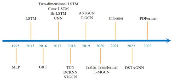
Figure 2.
Timeline of deep learning-based prediction algorithms.
3. Problem Statement and Input Data Representation Methods
3.1. Traffic Data and Their Unique Characteristics
The first step in ensuring accurate traffic prediction is acquiring high-quality data primarily from various sources. These sources mainly include fixed sensors (such as traffic cameras, induction loops, and radar sensors), mobile sensors (such as GPS devices in vehicles and smartphone apps), public transit systems, traffic management centers, social media and online platforms, satellites, aerial imagery, and third-party data service providers. Fixed sensors collect information about vehicle flow, speed, and road occupancy. Mobile sensors provide data on vehicle location and moving speeds. Public transit system data include the positions of buses and subways, departure intervals, and passenger counts. Traffic management centers integrate real-time and historical traffic data. Social media and online platforms offer updates on traffic incidents and road conditions. Satellites and aerial imagery monitor large-scale traffic flow and vehicle density. Third-party data service providers provide comprehensive traffic data that has been preprocessed and analyzed. After obtaining these data, preprocessing steps such as data cleaning, handling outliers, and data integration are typically performed to improve data quality and relevance, providing reliable inputs for traffic prediction models. These high-quality data are the foundation for achieving accurate traffic predictions. To summarize, the unique characteristics of traffic data are as follows:
- Strong periodicity. Traffic data exhibit significant daily and weekly cycles. Typical patterns include morning and evening rush hours during weekdays and different traffic patterns on weekends. Seasonal variations, such as holiday traffic spikes, also exhibit periodicity.
- Spatial dependencies. While many time series involve only time, traffic data are inherently spatiotemporal. Due to the interconnected nature of road networks, the traffic conditions at one location can highly depend on the traffic conditions at nearby or distant locations.
- Non-stationarity. Traffic patterns change over time and are influenced by factors like urban development, changes in traffic regulations, or the introduction of new infrastructure. This non-stationarity means that the statistical properties of the traffic data (such as mean and variance) can vary, making modeling more challenging.
- Volatility. Traffic data can be highly volatile due to unexpected events such as accidents, roadwork, or weather conditions. These events can cause sudden spikes or drops in traffic flow that are not easily predictable with standard models.
- Heteroscedasticity. Traffic volume variability is not constant over time. It can vary significantly across different times of the day or days of the week, particularly increasing during rush hours and decreasing at night.
- Multivariate influences. Traffic conditions are influenced by a wide range of factors beyond just the number of vehicles on the road. Weather conditions, special events, economic conditions, and social media trends can affect traffic flow and congestion levels.
These unique traffic data characteristics make it challenging to model traffic data prediction. The general prediction model cannot be directly applied to the task of traffic data prediction. On the other hand, traffic data encompass both spatial and temporal dimensions. These datasets capture traffic events’ geographical locations (spatial) and corresponding timeframes (temporal). Integrating spatial coordinates and time stamps enables the analysis of traffic patterns, flow dynamics, and congestion over time and across different locations. This dual-dimensional nature renders traffic data inherently spatiotemporal. Thus, effective traffic data prediction must incorporate spatial and temporal dependencies within the dataset. By considering these interdependencies, the predictive models can more accurately capture the dynamic nature of traffic patterns, which are influenced by location-specific factors and temporal variations. Ignoring either dimension would undermine the predictive accuracy and reliability of the model.
3.1.1. Spatial Dependencies
To describe the spatial dependencies within traffic data, the representation can be primarily categorized into the following three ways.
- Stacked Vector
We can use domain knowledge to stack data from multiple related spatial units according to predefined rules to capture spatial dependency, forming a multi-dimensional vector. The data for each unit can include traffic flow, speed, density, etc. Through stacking, these vectors can simultaneously represent the traffic conditions of multiple geographic locations.
- Matrix/Grid Representation
To capture spatial dependencies, spatial data, such as points or areas within a traffic network (a traffic matrix is a two-dimensional matrix with its -th element denoting the amount of traffic sourcing from node and exiting at node ), are mapped onto a two-dimensional matrix or grid. In this matrix or grid, each row and column represents a specific geographic location, and each cell in the matrix contains the traffic data for that location. This treats spatial information as two-dimensional Euclidean data composed of geographic information, representing it like an image. This method can be called matrix-based representation or grid-based map segmentation. As shown in Figure 3, the city map is divided into a grid-based map format.
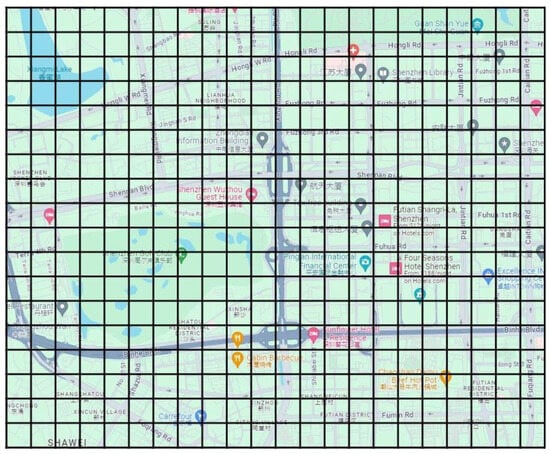
Figure 3.
Grid-based map segmentation in Shenzhen.
- Graph Representation
Compared to image data, traffic network data exhibit more complex spatial dependencies, primarily because these dependencies cannot be solely explained by Euclidean geometry. For example, traffic networks are inherently graph like rather than grid like. While image data naturally align into a regular grid where each pixel relates primarily to its immediate neighbors, traffic nodes (such as intersections and bus stops) connect in more complex patterns that often do not correspond to physical proximity.
A graph consists of multiple nodes and edges that connect these nodes. Each node represents a specific spatial unit. In the representation of a graph, a matrix of size of is commonly used to describe the complex relationships between nodes, where is the total number of nodes. This matrix is called an adjacency matrix , and its element () represents the connectivity status between the th and -th spatial units. These connections may involve distance, connectivity properties, and other more complex spatial relationships, often beyond simple Euclidean distance definitions.
3.1.2. Temporal Dependencies
Temporal dependencies are typically categorized into two main types in data representation: sequentiality and periodicity. Sequentiality represents the natural order of data over time, which in traffic prediction means that data are collected in chronological order, with each data point timestamped later than the previous one, similar to the stacked vector method for representing spatial dependencies, where consecutive temporal units are stacked into a single vector to indicate that temporally closer data are more related. Periodicity involves the recurring patterns displayed by data, such as daily cycles (peak and off-peak periods within a day) or weekly cycles (differences in traffic patterns between weekdays and weekends). Representing data with periodicity allows models to capture these regularly occurring patterns, enabling accurate predictions for similar future periods.
3.2. Common Forms of Input Representations
With the rapid development of intelligent transportation systems, advanced deep learning techniques, particularly RNNs and their variants, for analyzing and predicting time series data have become a hot research area. RNNs, due to their unique feedback structure, demonstrate significant advantages in capturing long-term dependencies within time series data. However, the performance of RNNs in traffic prediction depends on their algorithms and is heavily influenced by the methods used to represent input data.
Data representation methods play a pivotal role in model design and predictive performance. Different data representation formats, such as time series, grid sequences, or graph sequences, each possess distinct characteristics and advantages suitable for handling various types of traffic data. For example, time series methods emphasize the changes in traffic data over time, while grid sequences and graph sequences also concern spatial dependencies. Furthermore, applying sliding window techniques is particularly crucial for capturing time dependencies, as it allows for the inclusion of continuous sequences of historical data in the model, thereby enhancing prediction accuracy.
With the advancements in big data and computing capabilities, an increasing number of studies are now exploring the impact of different data representation methods on the performance of RNNs in traffic prediction. From essential time series forecasting to complex spatiotemporal data analysis, researchers are striving to identify the most effective data representation methods to improve the accuracy and efficiency of traffic prediction. This section concentrates explicitly on the traffic prediction task’s common input data representation methods. We aim to provide a comprehensive perspective to better utilize RNNs for traffic prediction by analyzing the latest research findings. Below, we will explore the relevant literature regarding three forms of input sequences: time series, matrix/grid-based sequences, and graph sequences. Table 1 summarizes these three types of forms of input representations.
3.2.1. Time Series
The data representation of a time series encompasses the organization and structure of the data points that describe the evolution of a quantity over time. It consists of two fundamental components: the time stamp or index and the corresponding data values. The time stamp indicates when each observation was recorded and can take various formats, such as dates, timestamps, or numerical indices representing time intervals. The data values represent the actual measurements or observations of the quantity of interest at each time stamp. Together, these components form a sequential series of data points that can be analyzed to identify patterns, trends, and relationships over time. Time series, , can be represented as , where represents the traffic state at time . Time series is a common way to represent traffic data. It emphasizes the importance of traffic patterns that change over time. For example, Rawat et al. [50] provided a comprehensive overview of time series forecasting techniques, including their applications in various fields. Furthermore, in traditional studies, RNNs only utilize the time series of traffic volume as input and do not incorporate any attribute information from the time series data, such as timestamps and days of the week. However, traffic volume varies depending on the time and day of the week. Therefore, in addition to the time series of traffic volume, attribute information can be used as input to enhance the prediction accuracy of RNN methods further. Tokuyama et al. [51] investigated the impact of incorporating attribute information from the time series of traffic volume on prediction accuracy in network traffic prediction. They proposed two RNN methods: the RNN–Volume and Timestamp method (RNN-VT), which uses timestamp information, and the RNN–Volume, Timestamp, Day of the week method (RNN-VTD), which utilizes both timestamp and day of the week information as inputs, in addition to the time series of traffic volume. Some studies have also considered the potential connections between traffic states and their contexts by integrating time series data with contextual factors. For instance, Lv et al. [52] used time series to represent the scenario of short-term traffic speed prediction, where these time series data represent the average speed of all vehicles during specific time intervals, aiming to accurately reflect the movement status of vehicles. They introduce Feature-Injected RNNs (FI-RNNs), a network that combines time series data with contextual factors to uncover the potential relationship between traffic states and their backgrounds. Some studies decompose time series data, such as Wang et al. [53], who used time series to represent traffic flow data in urban road networks. Specifically, the study addresses short-term traffic flow prediction in urban road networks and emphasizes the periodicity and randomness of traffic data. To handle these traffic data, the research is divided into two modules. The first module consists of a set of algorithms to process traffic flow data, providing a complete dataset without outliers through analysis and repair and offering a dataset of the most similar road segment pairs. The second module focuses on multi-time step short-term forecasting. Awan et al. [54] demonstrated that in addition to parameters related to traffic, other features associated with road traffic, such as air and noise pollution, can also be integrated into the input. This study uses time series to represent road traffic data in the city, specifically focusing on the correlation between noise pollution and traffic flow to predict traffic conditions. The noise pollution data provide additional indicators of traffic density and traffic flow. These time series integrate changes in road traffic flow and the associated levels of noise pollution, revealing the interaction between traffic flow and noise pollution. Then, an LSTM model is used to predict traffic trends. Traditional time series forecasting models perform poorly when encountering missing data in the dataset. Regarding temporal dependencies, all roadways undergo seasonal variations characterized by long-term temporal dependencies and missing data. Traditional time series forecasting models perform poorly when encountering missing data in the dataset.

Table 1.
Summary of different input representations.
Table 1.
Summary of different input representations.
| Input Representations | Reference | Techniques |
|---|---|---|
| Time Series | [51] | RNN |
| [52] | RNN | |
| [53] | LSTM | |
| [54] | LSTM | |
| Matrix/Grid-based Sequence | [55] | ResNet |
| [56] | LSTM + CNN | |
| [57] | LSTM + CNN | |
| [58] | LSTM + CNN | |
| Graph-based Sequence | [59] | RNN + GNN |
| [60] | LSTM + GNN | |
| [61] | GRU + GCN | |
| [62] | GAT + Attention | |
| [63] | GCN + Attention |
3.2.2. Matrix/Grid-Based Sequence
We previously discussed the spatial dependencies of traffic data, which revealed the mutual influence of traffic conditions between different locations. To effectively capture this spatial relationship, the method of dividing a map into grids in Euclidean space can be used. Specifically, the map is divided into many uniform small areas, with each grid representing a specific area on the map. This way, the map’s location information is transformed into a two-dimensional matrix or grid structure. In this structure, each cell of the matrix or grid contains traffic information for a particular area and simulates the spatial proximity of the real world between cells. Additionally, the traffic matrix (TM) refers to a specific application scenario, namely, the representation of traffic flow between different nodes (such as intersections, city areas, etc.) in a network. Data processed in this manner are referred to as a grid-based sequence, as shown in Figure 4a. The grid-based sequence, , consisting of rows and columns is spread over time steps, and it can be represented as , where represents a two-dimensional matrix indicating the traffic state of all grids at time . Zhang et al. [55] divided the city into equally sized grid areas, with each grid cell capturing the inflow and outflow traffic volume of pedestrian flows. Inflow is defined as the total traffic volume entering an area within a given time interval. In contrast, outflow is defined as the total traffic volume leaving the area within the same time interval. Matrices at each time step are stacked to form a three-dimensional tensor, representing the temporal sequence of pedestrian flow volumes. Yao et al. [56] represented city roads in a grid format, where each grid cell captures taxi demand. The constructed matrix is in a single tensor form. They built a matrix sequence where each matrix represents the city’s taxi demand at different time steps. Bao et al. [57] constructed a grid-based matrix sequence for short-term bike sharing demand. Specifically, they partitioned the surveyed areas of Shanghai into a grid of 5 × 5 cells, aggregating the trip data of bicycles in Shanghai (including start timestamps, start geolocations, end timestamps, end geolocations, etc.), as well as collecting weather and air quality data, based on grid cells. The data for each time step are integrated into a matrix, with each matrix element containing comprehensive data for the corresponding grid cell; over time, these matrices are arranged in chronological order to form a matrix sequence. Zhou et al. [58] divided the city into several grids and proposed a parameter to control the grid width. This study suggests that the pickup demands from certain locations at the previous time step will affect the dropoff demands at the next time step. Subsequently, all data are mapped to the grids, and each grid’s pickup and dropoff demands are aggregated for each time interval. Demand matrices are generated for each time interval, quantifying the number of pickup and dropoff demands occurring within each grid.
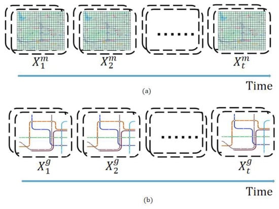
Figure 4.
Two representations of spatiotemporal traffic data: (a) a simple schematic diagram of a grid-based sequence data representation, representing a sequence of traffic data changing over time; (b) a simple schematic diagram of a graph-based sequence data representation, representing a sequence of traffic data changing over time.
3.2.3. Graph-Based Sequence
After discussing the grid-based sequence data representation, it is worth noting that much traffic data are collected based on complex traffic networks and their spatial dependencies closely rely on the topology of these networks. Therefore, to accurately describe and capture the spatiotemporal big data characteristics existing in traffic networks, we need a data representation method that reflects the network properties at each time step, namely, graph-based sequence data representation, as shown in Figure 4b. In this representation, each sequence element is treated as a graph at each time step, and the relationships or dependencies among elements are represented by time series. The graph-based sequence is , where each is a graph representing the state of the entire traffic network at time . Each graph can be further defined as , where is the set of nodes in the graph, with each node representing a specific location in the traffic network. is the set of edges in the graph, representing the connections between nodes. is the adjacency matrix. This approach is particularly suitable for capturing complex graph-based spatial and temporal data dependencies. It is widely used in multiple tasks in machine learning and data mining, such as sequence classification, clustering, and prediction.
In recent years, significant progress in traffic prediction research has been made using graph sequences as input sequences. Roudbari et al. [59] used graph-based sequence data to characterize road network traffic speed over time. These data encompass recorded journey information for road segments, considering the road network as a unified graph where nodes represent road segments and edges denote connections between these segments. Variable features are integrated into node information through an adjacency matrix, while static features are regarded as edge information. Their study categorized travel times for road segments, creating temporal lists on adjacent nodes sharing the same road segment, thus establishing a speed matrix that records speed variations for all road segments. Finally, the adjacency and speed matrices are combined to form graph-based sequential data. Additionally, Lu et al. [60] used graph-based sequence data to characterize vehicle speeds over a period in urban road networks. Specifically, the road network structure is constructed as a graph based on map data, with special consideration for the accessibility between different road segments. This not only reflects the physical structure of the roads but also accounts for actual traffic flow conditions, like when a road segment is temporarily closed due to maintenance or a traffic accident. Their study computes the traffic speeds of different road segments at various time points using taxi trajectory data, which are then matched with the road network. Graph-based sequence data are formed by continuously constructing these road traffic speed graphs. Wang et al. [61] used graph-based sequence data to predict traffic flow in urban road networks. Specifically, the road network structure is constructed as a graph based on spatial–temporal data, with each node representing a traffic sensor and edges representing the correlations between sensors at different time steps. The study computes traffic flow data at various time points using real-time sensor readings, forming a sequence of graphs where each graph represents the traffic conditions at a specific time step. Jams et al. [62] utilized a data-driven graph construction scheme for traffic prediction. In their approach, nodes represent traffic sensors, and edges represent the correlations between sensor readings at different time points. They dynamically construct graphs by embedding sensor correlations in a latent attention space and generate them at each time step to form a sequence. Gu et al. [63] used graph-based sequence data to describe traffic flow over a period in urban traffic networks. They define the topological road network as a directed graph, where nodes represent detectors on the roads, and features, such as traffic flow and speed, are added to the nodes. Their study distinguishes between two types of graphs: static adjacency graphs and dynamic adjacency graphs. The static adjacency graph is constructed without relying on prior assumptions, simulating typical long-term spatial dependencies in traffic patterns, while the dynamic adjacency graph addresses short-term local dynamics, allowing relationships between nodes to adjust over time based on observed data. Timestamp information is effectively concentrated on historical time information using a multi-head self-attention mechanism. The graphs of consecutive time steps (static and dynamic adjacency graphs) are concatenated to form a graph sequence encompassing both spatial and temporal dimensions. This way, each graph at a time node not only contains the traffic state at that moment but also reflects changes in the relationships between nodes from one time step to the next through the variations in the edges of the dynamic adjacency graph. Importantly, they embed learnable time and space matrices into the input graph-based sequence, ultimately becoming the model’s input.
3.2.4. Sliding Window
The size of the sliding window is often a critical parameter that needs to be adjusted in forecasting research. Using RNNs for the prediction process allows for recognizing and learning data patterns within time series data. However, the presence of fluctuations in the data can make it challenging to understand these data patterns. The dataset utilized in the study by Sugiartawan et al. [64] records the visitor volume at each time point over ten years, showcasing the changes in visitor visitation to attractions over time, characterized by linear trends and periodic fluctuations. The study employs 120 data vectors for prediction processing, representing tourism visitation data for 120 months. Based on these 120 data vectors, the study conducts multiple experiments and determines a window size setting of 3, meaning each window contains data from three time steps. In the study, the window moves forward one time step at a time, and ultimately, the model predicts the visitor volume at the next time point based on the visitor count data from the past three time points. Like other deep learning models, GRUs require careful adjustment of the sliding window size to optimize predictive performance. To explore this tedious process, in the study conducted by Basharat Hussain et al. [65], they continuously adjust the input window size of the GRU model to enhance its predictive capabilities. The original data are derived from average traffic flow data collected at 5 min intervals. Through experimentation, the researchers tested various window sizes (3, 6, 12, 18, 24) to determine which size most effectively improves the performance of the GRU model. In a GRU model configured with 256 neurons in the first layer and two hidden layers containing 64 and 32 neurons, respectively, they find that a window size of 12 yielded the best predictive performance. Lu et al. [66] combined the ARIMA model and LSTM for traffic flow prediction. In the ARIMA model, regression with a sliding time window is introduced, allowing the model to fit new input data for more accurate predictions continuously. This combined approach merges the projections of the two models through dynamic weighting, where the weights of each model in the final prediction are adjusted based on the standard deviation between the predicted results and the actual traffic flow at different time windows.
3.3. Problem Statement
Traffic prediction involves using historical traffic data to forecast future traffic conditions accurately. In the context of traffic data analysis, predictions are typically categorized into short-term, mid-term, and long-term predictions based on the forecast horizon. Short-term prediction involves forecasting traffic conditions over a horizon ranging from a few minutes to a few hours into the future. This type of prediction is crucial for real-time traffic management and control systems. Mid-term prediction refers to forecasting traffic conditions over a horizon extending from a few hours to several days. This type of prediction is used for planning and operational strategies that require an understanding of traffic patterns beyond immediate real-time needs. Long-term prediction involves forecasting traffic conditions over a horizon extending from several days to several months or even years. This type of prediction is important for strategic planning, infrastructure development, and policymaking [67]. In this review, short-term traffic prediction problems are our focus. Due to the diversity and complexity of traffic data, the traffic prediction tasks also vary. Therefore, a sufficiently generalized problem definition is needed to represent the short-term traffic prediction problem clearly.
Assume a spatial network with a set of sensors deployed, where each sensor records attributes (such as traffic flow, traffic speed, traffic occupancy, etc.) over timestamps. Thus, the observations of all sensors across all time points can be represented as a three-dimensional tensor, , and it can be represented as , where represents the attribute data of all sensors at timestamp . represents the exogenous factors that influence future traffic conditions, such as information on weather, holidays, big events, etc. Assume that the traffic prediction task requires predicting the traffic attributes for the next time steps based on the traffic attributes from the past time steps and exogenous factors ; the traffic prediction task can be defined as follows:
where is the method used for prediction. represents the model’s parameters, including all weights and biases in the network. is the prediction at time . This problem definition provides a clear and structured approach to utilizing various methods for traffic prediction, ensuring coverage of all relevant variables.
4. RNN Structures Used for Traffic Prediction
4.1. RNNs
RNNs are a class of iterative learning machines that process sequence data by cyclically reusing the same weights. This cyclical structure enables them to maintain a memory of previous data points using this accumulated information to process current inputs, thereby capturing temporal dependencies. Specifically, an RNN applies a transfer function to update its internal state at each time step. The general formula for this update is as follows:
Here, is identified as the input vector at time step and is the previous hidden state. is the weight matrix for the connections between the input at the current time step and the current hidden state. is the weight matrix for the connections between the previous hidden state and the current hidden state. and represent bias vectors. The function acts as the activation function.
The hidden state at each time step is updated using a combination of the current input and the previous hidden state . Weight matrix facilitates the incorporation of new information and weight matrix helps in transferring past learned information. and adjust the inputs and the state transition. The function , typically a non-linear activation function, is applied to introduce non-linearity into the system, enabling the network to capture complex patterns in sequential data.
4.2. LSTMs
Theoretically, RNNs are simple and powerful models, effectively training them poses many challenges in practical applications. One major issue is the problem of vanishing and exploding gradients. Gradient explosion occurs during training when the norm of gradients sharply increases due to long-term dependencies, growing exponentially. Conversely, the vanishing gradient problem describes the opposite phenomenon, where gradients for long-term dependencies rapidly diminish to near-zero levels, making it difficult for the model to learn long-range dependencies. To overcome these issues, the introduction of LSTM addresses the problem by employing gate mechanisms to maintain long-term dependencies while mitigating gradient problems. These gate control systems include input gates, forget gates, and output gates, which work together to regulate information flow, retention, and output precisely.
The basic formulas for LSTM are as follows:
where represents the input vector at time step . represents the hidden state vector at time step and will serve as part of the input for the next time step. , , and are the outputs of the forget gate, input gate, and output gate. is the candidate layer at time step , representing potential new information that might be added to the current cell state. is the LSTM’s internal state, containing the network’s long-term memory. , , , and are the weight matrices for the forget gate, input gate, output gate, and candidate layer. , , , and are the bias vectors for the forget gate, input gate, output gate, and candidate layer, respectively. is the sigmoid activation function used for gating mechanisms and is the hyperbolic tangent activation function used for non-linear transformations.
The forget gate decides which information to discard by using a sigmoid function that outputs values between 0 and 1 for each component in the cell state, where 1 means “retain this completely” and 0 means “discard completely”. Simultaneously, the input gate and a candidate layer decide which new information is stored by creating a vector of new candidate values. The cell state is then updated by combining the old state, multiplied by the output of the forget gate, with the new candidate values scaled by the output of the input gate. Lastly, the output gate together with the cell state passed through a function determines the next hidden state , filtering the information to the output. This mechanism enables LSTMs to handle vanishing gradients and learn over extended sequences effectively.
4.3. GRUs
The GRU, as another prominent gated structure, was initially proposed by Cho et al. [68]. The GRU was proposed primarily to optimize the complexity and computational cost of LSTMs. While LSTMs are powerful, their structure includes three gates and a cell state, making the model complex and parameter heavy. The GRU simplifies the model structure by merging the forget gate and input gate into a single update gate, reducing the number of parameters and improving computational efficiency. Additionally, the GRU does not have a separate cell state; it operates directly on the hidden state, simplifying the flow of information and memory management. These improvements enable the GRU to efficiently handle tasks requiring capturing long-term dependencies while remaining a powerful model choice. The propagation formulas of the GRU are as follows:
Here, is the output of the update gate and is the output of the reset gate. , , and are the weight matrices for the update gate, reset gate, and candidate layer. , , and are the bias vectors for the update gate, reset gate, and candidate layer.
The GRU operates by effectively balancing the retention and introduction of new information in time series data. The update gate output controls the extent to which the previous hidden state is retained. The reset gate output dictates the influence of on the candidate’s hidden state . The candidate’s hidden state is obtained by applying the tanh activation function to the linear combination of the reset gate-adjusted previous hidden state and the current input. The final hidden state results from a linear combination of the previous hidden state, controlled by the output of the update gate, and the new candidate hidden state. The weight matrix is used to generate the candidate state, while the bias adjusts its bias. Thus, the GRU can effectively update its state, capturing long-term dependencies in time series data.
Figure 5 shows a comparison between the structures of the RNN and its variants. The RNN represents the simplest form, showing a single recurrent layer; the distinction of the LSTM lies in the introduction of three types of gates (input, forget, and output gates), which allow the network to selectively remember or forget information and a cell state that helps maintain long-term dependencies, aiming to overcome the common problem of vanishing gradients seen in simple RNNs. The GRU merges the LSTM’s input and forget gates into a single update gate and combines the cell state and hidden state into a unified mechanism. Overall, this diagram clearly explains how different RNNs and their variants process information to handle sequential data.
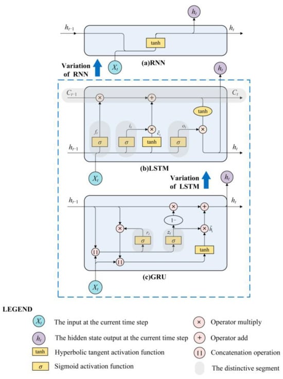
Figure 5.
Comparison of RNN, LSTM, and GRU neural network structures.
4.4. Hybrid Models Including RNN Techniques
In the field of traffic prediction, RNNs and their variants, such as LSTMs and GRUs, are widely adopted due to their excellent performance in handling time series data. However, as the complexity of traffic data continues to increase, models relying solely on RNNs are no longer sufficient to meet prediction requirements entirely. To further enhance prediction accuracy and effectively address the complexities of traffic data, researchers are beginning to explore methods that combine RNNs with other mechanisms and models. These methods may include but are not limited to combining RNNs with traditional machine learning (ML) techniques, CNNs, GNNs, and attention mechanisms aimed at achieving better results in traffic prediction tasks, as shown in Table 2.
4.4.1. RNNs + Traditional ML Techniques
As mentioned earlier, classical traffic flow prediction methods based on traditional ML techniques include K-NN and SVR. Some scholars have endeavored to combine these methods with the RNN family for traffic prediction. For example, Luo et al. [69] proposed a spatiotemporal traffic flow prediction method combining K-NN and LSTM. K-NN is used to select neighboring stations most relevant to the test site to capture the spatial characteristics of traffic flow. At the same time, LSTM is employed to explore the temporal variability of traffic flow. The experimental results show that this model outperforms some traditional models in predictive performance, with an average accuracy improvement of 12.59%. In comparison with combining with the LSTM model, Zhou et al. [70] proposed a traffic flow prediction method based on the K-NN and GRU. This method calculates spatial correlations between traffic networks using Euclidean distance and captures the time dependency of traffic volume through the GRU. The experimental results demonstrate a significant improvement in the prediction accuracy of this model compared to traditional methods. The K-NN method exhibits good predictive performance in simple scenarios. However, due to its non-sparse nature, it may struggle to handle traffic scenarios with significant variations. Tong et al. [71] utilized an optimized version of SVR as a traffic flow prediction method. They apply Particle Swarm Optimization (PSO) to optimize the parameters of SVR, thereby enhancing the prediction system’s performance. Given the complex non-linear patterns of traffic flow data, Cai et al. [72] proposed a hybrid traffic flow prediction model combining the Gravitational Search Algorithm (GSA) and SVR model. The GSA is employed to search for the optimal SVR parameters, and this model demonstrates good performance in practice.
Table 2.
Summary of different hybrid models.
Table 2.
Summary of different hybrid models.
| Hybrid Models | Reference | Techniques |
|---|---|---|
| RNNs + Traditional ML Techniques | [69] | LSTM + K-NN |
| [70] | GRU + K-NN | |
| RNNs + CNNs | [73] | LSTM + CNN |
| [74] | LSTM + CNN | |
| RNNs + GNNs | [42] | GRU + GCN |
| [75] | LSTM + GNN | |
| [76] | LSTM + GNN | |
| RNNs + Attention | [77] | LSTM + Attention |
| [78] | LSTM + Attention | |
| [79] | LSTM + Attention | |
| [80] | RNN + GNN + Attention | |
| [81] | GRU + GCN + Attention |
4.4.2. RNNs + CNNs
Researchers have gradually recognized the importance of spatial dependency, and the combined use of RNNs and CNNs in addressing spatiotemporal data issues, particularly in traffic flow prediction in the Euclidean-based space, has become an important research direction. This fusion method fully leverages the advantages of RNNs in handling time series data and the efficiency of CNNs in processing spatial features. RNNs are particularly suitable for handling time series data because they can capture the temporal dynamic characteristics and long-term dependencies in the data. However, RNNs have limited capability in dealing with high-dimensional spatial data. CNNs effectively identify and extract local features from high-dimensional spatial data, such as images and videos. Still, they do not directly handle dynamic information in time series data. Therefore, combining RNNs and CNNs can achieve more comprehensive and accurate modeling and prediction of spatiotemporal data. Figure 6 shows an example of a hybrid RNN and CNN model.
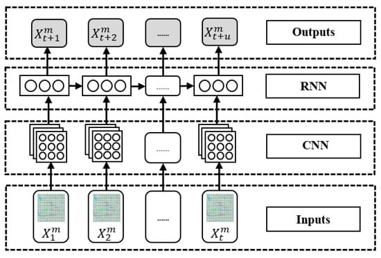
Figure 6.
Example of a hybrid RNN and CNN model.
Ma et al. [33] transferred the application of CNNs from images to the field of traffic prediction, forecasting large-scale transportation networks by utilizing spatiotemporal traffic dynamics transformed into images. This method integrates the spatial and temporal dimensions of traffic data into a unified framework, involving the conversion of traffic dynamics into a two-dimensional spatiotemporal matrix, fundamentally treating traffic flow as images. This matrix captures the intricate relationships between time and space in traffic flow, allowing for a more nuanced analysis of traffic patterns. Yu et al. [73] proposed an innovative approach for predicting traffic flow in large-scale transportation networks using Spatiotemporal Recurrent Convolutional Networks (SRCNs). The particular distinction of this method lies in transforming network-wide traffic speeds into a series of static images, which are then employed as inputs for the deep learning architecture. This image-based representation allows for a more intuitive and effective capture of the complex spatial relationships inherent in traffic flow across the transportation network. Empirical testing on a Beijing transportation network comprising 278 links further demonstrated the effectiveness of this method. Due to the potential variation in spatial dependencies between different locations in the road network over time and the non-periodic nature of temporal dynamics, Yao et al. [74] proposed a novel Spatial–Temporal Dynamic Network (STDN) for traffic prediction. This approach utilizes a flow gating mechanism to track the dynamic spatial similarity between regions, enabling the model to understand how traffic flows between areas change over time, which is crucial for accurately predicting future traffic volumes. Additionally, they employ a periodically shifted attention mechanism to handle long-term periodic information and time offsets. This allows the model to account for subtle variations in daily and weekly patterns, such as shifts in peak traffic times, thereby enhancing prediction accuracy.
4.4.3. RNNs + GNNs
When constructing deep learning spatiotemporal traffic prediction models, it is necessary to consider the characteristic graph structure of many transportation networks. Generally, passenger flow activities occur on specific transportation networks rather than simple Euclidean spaces. Modeling with non-graph structures may result in the loss of useful spatial information. CNNs are typically used to handle data with Euclidean spatial structures, such as regular grids. However, for non-Euclidean spaces, such as graph-structured data, the utility of CNNs is not as evident. To explore the spatial properties of non-Euclidean transportation networks, some scholars have adopted mathematical graph theory approaches, modeling transportation networks as graphs. This approach effectively depicts the connectivity between traffic nodes and opens new avenues for introducing convolutional operations. In recent years, GNNs have been widely employed to capture spatial correlations in transportation networks. Figure 7 shows an example of a hybrid RNN and GNN model.

Figure 7.
Example of a hybrid RNN and GNN model.
Zhao et al. [42] proposed a T-GCN model, which integrates the advantages of GCNs and GRUs. This model can simultaneously capture the spatial and temporal dependencies of traffic data. Furthermore, it incorporates encoder–decoder architecture and temporal sampling techniques to enhance long-term prediction performance. Wang et al. [75] proposed a novel spatiotemporal GNN for traffic flow prediction, which comprehensively captures spatial and temporal patterns. This framework provides a learnable positional attention mechanism, enabling effective information aggregation from adjacent roads. Additionally, modeling traffic flow dynamics to leverage local and global temporal dependencies demonstrates strong predictive performance on real datasets. Related studies also aim to reduce the data volume processed by neural networks to improve accuracy. For example, Bogaerts et al. [76] proposed a hybrid deep neural network based on a GNN and LSTM. Additionally, they introduced a time-correlation-based data dimensionality reduction technique to select the most relevant sets of road links as inputs. This approach effectively reduces the data volume, enhancing prediction accuracy and efficiency. The model performs well in short-term traffic flow prediction and exhibited good predictive capability in forecasting four-hour long-term traffic flow. Moreover, the proposed time correlation-based data dimensionality reduction technique effectively addresses prediction problems in large-scale traffic networks.
4.4.4. RNNs + Attention
Accurate traffic prediction optimizes road network operational efficiency, enhances traffic safety, and reduces environmental pollution. In recent years, with the development of deep learning methods, RNNs have been widely applied in traffic prediction due to their excellent ability to handle temporal data. Meanwhile, introducing attention mechanisms further improves the model’s capability to capture temporal and spatial dependencies. Figure 8 shows an example of a hybrid RNN and attention model.
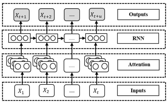
Figure 8.
Example of hybrid RNN and attention models.
The STAGCN model proposed by Gu et al. [63] combined static and dynamic graphs to accurately capture spatial dependencies in traffic networks. Additionally, the model introduces gated temporal attention modules to effectively handle long-term dependencies in time series data, thereby improving traffic prediction accuracy. Some scholars have improved training efficiency by introducing attention mechanisms on top of LSTM; for example, Qin et al. [77] integrated attention mechanisms to enhance training efficiency by simplifying the structure of LSTM networks while focusing on the most influential features for current predictions. This approach has shown superior performance and speed over traditional LSTM and RNN models on multiple public datasets. Similarly, Hu et al. [78] improved the LSTM-RNN by introducing attention mechanisms and developed a short-term traffic flow prediction model. This model demonstrates efficiency and accuracy in practical applications with real traffic flow data, confirming the effectiveness of attention mechanisms in enhancing traffic prediction performance. The SA-LSTM model proposed by Yu et al. [79] utilized self-attention mechanisms, effectively addressing the vanishing gradient problem and accurately capturing the spatiotemporal characteristics of traffic information. The superiority of this model is demonstrated in experiments on Shenzhen road network data and floating car data, showcasing the potential of self-attention mechanisms in improving traffic prediction accuracy. Additionally, some scholars, both domestically and abroad, have combined dynamic spatiotemporal graph recurrent networks with attention mechanisms. For instance, the Dynamic Spatiotemporal Graph Recurrent Network (DSTGRN) model proposed by Zhao et al. [80] integrated spatial attention mechanisms and multi-head temporal attention mechanisms by encoding road nodes, providing a fine-grained perspective for modeling the temporal dependencies of traffic flow data. This model surpasses its baseline models in prediction accuracy, demonstrating the potential application of dynamic graph networks in traffic prediction. Tian et al. [81] effectively captured the spatiotemporal characteristics of road conditions and achieved precise traffic speed prediction by combining the GCN and GRU and introducing multi-head attention mechanisms. Testing results on two real datasets demonstrate the superior performance of this model, further validating the application value of multi-head attention mechanisms in traffic prediction.
5. Sub-Areas of Traffic Prediction Applications Using RNNs
Various applications based on traffic prediction are developed to achieve smart transportation. This review investigates seven widely used applications: traffic flow prediction, passenger flow prediction, OD demand prediction, traffic speed prediction, travel time prediction, traffic accidents and congestion prediction, and occupancy prediction. Furthermore, these applications heavily rely on the performance of traffic prediction technology. Table 3 summarizes traffic prediction methods proposed in these seven fields of application and whether they consider temporal and spatial dependencies of traffic data.
5.1. Traffic Flow Prediction
Traffic flow prediction involves estimating the number of vehicles traversing a specific road segment within a certain timeframe. It is crucial for transportation planning and management because it allows for the optimization of traffic signals, better planning of road maintenance, and effective real-time traffic management. This, in turn, leads to reduced congestion, improved fuel efficiency, shorter travel times, enhanced safety, and increased overall reliability of the transportation network. The field of traffic flow prediction has witnessed significant advancements in recent years, particularly with the utilization of RNNs and their variants, such as LSTMs and GRUs. These methods have shown promise in accurately predicting traffic flow patterns, surpassing traditional approaches like ARIMA models.
The literature demonstrates a growing interest in harnessing deep learning techniques for traffic flow prediction, focusing on enhancing prediction models’ performance and accuracy. Fu et al. [30] introduced LSTM and GRU neural network methods for traffic flow prediction, showcasing their superiority over ARIMA models. Their work highlights the potential of RNN-based deep learning methods in capturing the intricate patterns inherent in traffic flow data. Similarly, Zheng et al. [82] proposed a hybrid deep learning model featuring attention-based Conv-LSTM networks, which aims to automatically extract intrinsic features of traffic flow data, resulting in improved prediction performance. This underscores the effectiveness of advanced deep learning architectures for traffic flow prediction. Shu et al. [83] explored using an enhanced GRU neural network, known as the Bi-GRU prediction model, for short-term traffic flow prediction. Their study provides insights into the characteristics of this model and its effectiveness in addressing short-term traffic flow prediction tasks. Chen et al. [84] also introduced the Attentive Attributed Recurrent GNN (AARGNN) for traffic flow prediction, incorporating GNNs to consider multiple dynamic factors. This multi-faceted approach illustrates the increasing complexity of models designed to capture the dynamic nature of traffic flow. Huang et al. [85] proposed a multi-attention predictive RNN (MAPredRNN), which leverages dynamic spatiotemporal data fusion for traffic flow prediction. Their approach emphasizes effectively fusing spatiotemporal data for accurate traffic flow prediction. Moreover, Liu et al. [86] conducted a comparison between the LSTM model and traditional RNNs and demonstrated the LSTM model’s higher prediction accuracy and effectiveness in traffic flow prediction. Previous studies have often integrated spatiotemporal prediction models with GNNs and temporal processing modules to capture the spatiotemporal dependencies of traffic networks. However, they have encountered issues related to static spatial connectivity and the loss of global temporal dependency information. To address these challenges, Zhao et al. [80] introduced the DSTGRN, which utilizes spatial and temporal attention mechanisms for fine-grained modeling, improving accuracy in predicting traffic flow data. RNNs and their variants, like LSTMs, are designed to model long-term temporal correlations in sequences. However, multi-regime models consider multiple states in the traffic system, each with distinct characteristics, necessitating separate models. Agnimitra Sengupta et al. [87] proposed a hybrid Hidden Markov LSTM model that combines their strengths, improving traffic flow prediction, especially in complex and non-stationary scenarios. Due to various factors, such as weather, accidents, and road control affecting traffic flow, it exhibits significant and irregular fluctuations. This challenge is particularly pronounced when predicting traffic flow trends at the minute and hour levels. To address this issue, Wang et al. [88] proposed a sequential model called an LSTM–Light Gradient-Boosting Machine (LSTM-LightGBM) for hourly traffic flow prediction, taking into account the temporal, periodic, and spatial features of traffic flow. The model leverages LSTM to capture temporal characteristics and LightGBM to capture spatial and periodic features. Testing on the Chicago traffic dataset demonstrated that the LSTM-LightGBM model outperforms other baseline models, with a potential reduction in the RMSE of up to 50%, considering that weather factors are crucial for traffic flow prediction. However, existing models typically utilize shallow prediction techniques, resulting in suboptimal accuracy when accounting for external factors, such as weather. Zhou et al. [89] introduced an enhanced LSTM model with an attention mechanism for short-term traffic flow prediction that considers weather factors. Experiments conducted on the Caltrans PeMS traffic dataset demonstrate that the proposed model outperforms the original LSTM model, reducing its Mean Absolute Percentage Error (MAPE) by 23.36%. Yang et al. [90] introduced a novel short-term traffic flow and speed prediction approach. The model effectively combines attention mechanisms, CNNs, and GRUs within a multi-task learning framework. This innovative method demonstrates enhanced accuracy and robustness in predicting traffic conditions in diverse urban and highway scenarios, although it requires substantial computational resources and complex data processing. The literature presents a diverse array of approaches for traffic flow prediction, encompassing advanced deep learning architectures and incorporating multiple dynamic factors and spatiotemporal data fusion. These developments underscore the ongoing progress and innovation in the field as researchers strive to enhance the accuracy and reliability of traffic flow prediction.
5.2. Passenger Flow Prediction
Passenger flow prediction involves forecasting the number of passengers expected to use a particular transportation service or facility over a specified period. It is significant for transportation as it aids in optimizing the allocation of resources, such as scheduling of transit services, staffing, and facility management. Accurate predictions enhance operational efficiency, reduce waiting times, improve service quality, and improve capacity management. This results in increased passenger satisfaction and a more reliable and efficient transportation system. Several traffic prediction techniques estimate passenger flow at different traffic nodes, such as bus stops, subway stations, and airports.
Lin et al. [91] studied the application of the RNN and LSTM in passenger traffic forecasting and demonstrated their performance in experiments. The advantage is that the RNN and LSTM show superior performance compared to other models, but there may be challenges in handling long time series data. Maazoui et al. [92] explored the application of LSTM for passenger flow prediction on railroad networks. They find that LSTM slightly outperforms ARIMA and other statistical models in terms of Mean Absolute Error (MAE) at railroad stations but performs poorly in train line prediction. Izudheen et al. [93] proposed an LSTM-based model for predicting passenger traffic at subway stations. This model can comprehensively consider multiple factors to enhance prediction accuracy, but it requires high data diversity. Wen [94] demonstrated the advantages of the Genetic Algorithm-optimized LSTM (GA-LSTM) in terms of passenger traffic forecasting accuracy. The benefit is its superior accuracy compared to non-optimized RNNs, but the drawback is that the parameter optimization process may be complex. Zhai et al. [95] used the DCRNN model to perform excellently in bus passenger traffic forecasting, achieving a 5% improvement in accuracy compared to traditional RNNs. Sun [96] conducted comparative studies and found that the CNN-LSTM outperformed pure LSTMs in subway station passenger flow prediction despite their higher complexity and computational requirements. Xu et al. [97] successfully predicted the passenger flow of attractions through a GCN-RNN model using passenger flow data from neighboring bus and metro stations. The model’s strength lies in its utility, but its dependence on region-specific traffic data limits it. Wang et al. [98] introduced a novel Residual RNN Channel Spatiotemporal Graph Convolution Network (RRC-STGCN) for predicting passenger traffic at railway stations. The model outperforms several baseline models, but its implementation is relatively complex, requiring a substantial amount of data for training.
RNNs and their variants are increasingly used in passenger traffic prediction, and they show significant advantages in processing time series data. However, these models usually require large amounts of data for training and may exhibit different strengths and weaknesses in various application scenarios.
5.3. OD Demand Prediction
Short-term OD demand prediction estimates the number of trips between different origins and destinations within a transportation network. Because of the high dimensionality and sparsity of the data, accurately determining OD demand is significantly more difficult than estimating traffic/passenger flow. This prediction is significant for transportation planning and management, providing critical insights into travel patterns and demands. It helps optimize route planning, enhance public transit scheduling, design infrastructure projects, and improve traffic management strategies. Accurate OD demand prediction ensures better resource allocation, reduces congestion, improves travel times, and enhances overall system efficiency and reliability. Islam et al. [99] proposed a complex prediction model that integrates LSTMs and RNNs. The study emphasizes the model’s efficiency across different seasons and validates its performance using various error metrics, but it faces challenges with complexity and data requirements. Toqué et al. [100] presented an innovative LSTM approach to predict dynamic OD matrices in a subway network. The advantage of this method is its reliable short-term prediction of OD pairs. Still, it requires a substantial amount of smart card data for training and additional data from nearby transportation systems to enhance prediction accuracy, which can be considered a drawback. Nejadettehad et al. [101] utilized three types of RNNs, including simple RNN units, GRUs, and LSTMs, to predict short-term traffic OD demand. The results indicate that the simpler RNNs, such as simple recurrent units and GRUs, outperform LSTMs regarding accuracy and training time. Ride-hailing services have witnessed dramatic growth over the past decade but have raised various challenging issues, one of which is how to provide a timely and accurate short-term prediction of supply and demand. While the predictions for zone-based demand are extensively studied, much less effort is paid to the predictions for OD-based demand (namely, demand originating from one zone to another). However, OD-based demand prediction is even more important and worth further exploration. Feng et al. [102] introduced a model called the Multi-Task Matrix Factorized Graph Neural Network (MT-MF-GCN), which combines the GCN and matrix factorization modules. This model is used to predict both zone-based and OD demand simultaneously in ride-hailing services, and it demonstrates outstanding performance in real-world testing. Wang et al. [103], in contrast to previous studies on ride-hailing demand prediction that primarily focused on inflow or outflow demands of each zone, proposed a Conditional Generative Adversarial Network with a Wasserstein divergence objective (CWGAN-div) for predicting ride-hailing OD demand matrices. They utilize interpretable conditional information to capture external spatiotemporal dependencies, ultimately guiding the model to generate more precise results. RNNs are one of the most popular methods for predicting OD demand in ride-hailing services. However, due to the diversity of these networks, the question of which type is most suitable for this task still needs to be solved. Compared to road systems, the OD distribution in urban rail transit exhibits distinct characteristics, including high dimensionality and sparsity, posing significant challenges for data-driven prediction models. While existing research has made some progress in mining spatiotemporal features, current models still lack objectivity when considering prediction framework embedding, multi-source data fusion, and integration of spatiotemporal feature mining. Gu et al. [104] proposed a deep learning framework based on a multi-factor fusion channel-wise attention mechanism. This framework can capture the intrinsic relationships between inter-station, date attributes, external factors, and passenger flow distribution’s high-level spatial correlations and further abstract spatiotemporal features using convolutional LSTM to generate prediction results. The study demonstrates that this model achieves higher network-level prediction accuracy.
5.4. Traffic Speed Prediction
Traffic speed prediction involves forecasting the average speeds of vehicles on specific road segments over a given period. This prediction is significant for transportation because it is crucial in traffic management, road safety, and infrastructure planning. By accurately predicting traffic speeds, authorities can optimize traffic signal timings, manage congestion, and provide real-time traffic information to drivers. This leads to improved travel times, reduced fuel consumption, and enhanced overall efficiency and safety of the transportation network. Deep learning models have been developed to accurately forecast traffic speed based on different data sources, such as remote microwave sensor data, network-wide traffic patterns, and spatiotemporal correlations. Among the range of deep learning models applied to this problem, RNNs, LSTMs, and GRUs have emerged as popular choices due to their ability to capture temporal dependencies effectively.
Ma et al. [28] proposed an LSTM neural network for traffic speed prediction using remote microwave sensor data, which demonstrates superior prediction performance in terms of accuracy and stability. This work lays the foundation for the application of LSTM networks in traffic speed prediction. In a different direction, Kim et al. [105] introduced structural RNNs for traffic speed prediction, demonstrating the potential benefits of embedding topological information in the road network to improve the learning process of traffic features. Timely and accurate traffic speed prediction is essential for traffic management, but existing methods face challenges in feature extraction from large-scale traffic data. Cui et al. [106] further advanced this research by introducing a deep bidirectional and unidirectional LSTM for network-wide traffic speed prediction. The study shows that a deep Bi-LSTM neural network achieves superior prediction performance for the entire traffic network. Similarly, Lv et al. [107] presented the LC-RNN model, which integrates the RNN and CNN to achieve more accurate traffic speed prediction. This approach highlights the potential benefits of combining different neural network architectures for this task. Ma et al. [108] also introduced a hybrid spatiotemporal feature selection algorithm of a CNN-GRU model for short-term traffic speed prediction, showcasing the importance of combining spatial and temporal features for accurate predictions. Abdelraouf et al. [109] proposed an attention-based multi-encoder–decoder neural network for freeway traffic speed prediction, leveraging convolutional LSTMs to capture spatiotemporal relationships of multiple input sequences. Their focus on capturing spatiotemporal relationships through attention mechanisms further advanced the state of the art in traffic speed prediction. Hu et al. [110] proposed a hybrid deep learning approach for large-scale traffic speed prediction. The model comprises a Conv-LSTM module, an attention mechanism module, and two Bi-LSTM modules. The introduction of the attention mechanism module enhances Conv-LSTM’s performance by automatically capturing the importance of different historical periods and assigning corresponding weights. Additionally, two Bi-LSTM networks are designed to extract daily and weekly periodic features and capture trends from forward and backward traffic data. The model demonstrates good predictive performance but has a complex structure and slower prediction speed. Additionally, traditional traffic forecasting methods have significant limitations in capturing the dynamic characteristics of complex traffic networks. Therefore, there is a need for a predictive model that can efficiently represent spatial dependencies within the traffic network, model non-linear temporal dynamics simultaneously, and perform long-term forecasting for multiple time steps. Yin et al. [111] introduced a novel graph deep learning model that incorporated an attention mechanism for predicting traffic speeds in the network. It captures spatial dependencies through adjacency matrices and graph convolutions and learns temporal information using an RNN structure. The proposed attention-enabled model outperforms traditional forecasting models in prediction tasks.
These studies collectively demonstrate the significant advancements in traffic speed prediction using RNN-, LSTM-, and GRU-based models. The integration of different neural network architectures, attention mechanisms, and the consideration of spatiotemporal correlations have shown promising results in improving the accuracy and stability of traffic speed predictions. Overall, the literature indicates a growing consensus on the effectiveness of RNN variants for traffic speed prediction, with ongoing research focusing on enhancing the models’ ability to capture complex spatiotemporal patterns and network-wide traffic behaviors.
5.5. Travel Time Prediction
Travel time prediction involves estimating the duration required for a vehicle to travel between two points in a transportation network. This prediction is significant for transportation as it enhances route planning, improves the accuracy of navigation systems, and aids in traffic management. Providing reliable travel time estimates helps reduce uncertainty for travelers, optimizes logistics and delivery operations, and enhances the efficiency of public transit systems. Accurate travel time predictions contribute to reduced congestion, better resource allocation, and overall improved reliability and performance of the transportation network. There has been a growing interest in using RNNs in travel time prediction in recent years. One of the first successful attempts to apply RNNs in this field was made by Duan et al. [112]. They explore using LSTM neural network models specifically designed for travel time prediction, achieving remarkable results. In addition, Yuan et al. [113] proposed a deep feature extraction framework based on an RNN and DNN for bus dynamic travel time prediction, achieving greater efficiency than traditional machine learning models. Furthermore, a study by Ran et al. [114] introduced an LSTM-based method with an attention mechanism for travel time prediction, which demonstrates better accuracy and effective utilization of departure time. Another interesting work by Petersen et al. [115] used a convolutional LSTM neural network for multi-output bus travel time prediction, allowing the discovery of complex patterns not captured by traditional methods. Additionally, there have been efforts to combine different neural network models for travel time prediction. Ting et al. [116] proposed a deep hybrid model that combines the GRU and eXtreme Gradient Boosting (XGBoost) through linear regression, showcasing good prediction accuracy for freeway travel time. Moreover, due to the widespread availability of various observation data, such as vehicle data, data-driven travel time prediction methods have been rapidly advancing. In many existing large-scale network studies, speed time series data directly estimated from vehicle data are commonly used as inputs. However, in free-flow conditions, speed variations are not significantly influenced by the number of vehicles, making it challenging to depict the traffic conditions in this mode accurately. To address this issue, a study by Katayama et al. [117] introduced traffic density-based travel time prediction with GCN-LSTM, showcasing the superiority of density input in achieving early detection of traffic congestion and improving prediction accuracy. Following this, a study by Shen et al. [118] introduced the Traffic Trajectory Prediction Network (TTPNet). This novel neural network leverages tensor decomposition and graph embedding to achieve significantly better performance in travel time prediction. Furthermore, the processing capacity of traditional data processing and modeling tools needs to be improved for handling large-scale travel datasets. To overcome the challenges posed by massive data, Zhang [119] employed big data analytics engines, Apache Spark and the Apache Mixed Sparse Matrix Network (MXNet), for data preprocessing and modeling. They introduce a hierarchical LSTM model with attention mechanisms for network-level short-term travel time prediction, successfully forecasting unusual congestion and achieving the best prediction results at 30 min and 45 min horizons. Due to GRU’s ability to handle long-term traffic sequences, GRUs have been successfully applied to traffic prediction problems. However, existing GRUs do not consider the relationships between various positions in historical travel time sequences. Chughtai et al. [120] introduced an attention-based GRU model for short-term travel time prediction to address this issue, allowing the GRU to learn the relevant context in historical travel time sequences and update the weights of hidden states accordingly. Despite the need for complex data processing and significant computational resources, this model excels in handling noisy data.
In conclusion, applying RNNs, LSTMs, GRUs, and other neural network models for travel time predictions has shown significant progress and promising results, especially when combined with novel data processing techniques and attention mechanisms. Nevertheless, there is still potential for further research and innovation in this area.
5.6. Traffic Accidents and Congestion Prediction
Traffic accidents and congestion prediction involves forecasting the likelihood of traffic incidents and the occurrence of traffic jams on specific road segments. Traffic accidents and congestion prediction have been the subject of extensive research in artificial intelligence and machine learning. Various approaches, including RNNs, LSTMs, GRUs, and other deep learning models, have been employed to tackle the challenges of predicting traffic accidents and congestion.
Traffic accident prediction is to estimate the likelihood and severity of accidents by analyzing historical data and contextual data (e.g., weather, and road conditions). Its significance lies in enhancing road safety, optimizing traffic management, allocating emergency resources effectively, informing urban planning, guiding insurance risk assessments, raising public awareness, and reducing environmental impact. Sameen et al. [121] explored the use of RNNs for predicting the severity of traffic accidents. Their findings indicate that RNNs, within deep learning frameworks, hold promise in predicting injury severity in traffic accidents. Furthermore, Sameen et al. [122] demonstrated the superiority of deep learning models, like CNNs and RNNs, in predicting the severity of traffic accidents compared to traditional models. Their research emphasizes the advantages of leveraging deep learning techniques for more accurate and stable predictions. Similarly, Chui et al. [123] introduced an extended-range prediction model using the Non-dominated Sorting Genetic Algorithm III (NSGA-III) the optimized RNN-GRU-LSTM for driver stress and drowsiness, highlighting the potential of hybrid algorithms to enhance prediction performance. To accurately predict the number of traffic accidents and address road safety issues more effectively, Wang et al. [124] have proposed a time series prediction model based on LSTM and the attention mechanism. They use road traffic accident data and meteorological data from the city of Curitiba, Brazil, as their research dataset and improve the internal gating unit structure of the LSTM model. This model is used to fit and predict the traffic accident dataset. The results indicate that the prediction performance of the road traffic accident prediction model based on LSTM and the attention mechanism outperforms that of the classical LSTM model and SVR model; overall, this model has significant practical implications for enhancing road traffic management. Yu et al. [125] proposed a method called a Deep Spatiotemporal GCN (DSTGCN) for traffic accident prediction. The DSTGCN model combines the GCN for spatial data processing and the TCN for time series analysis, further exploring the spatial and temporal dependencies in traffic data. Experimental results show that the DSTGCN outperforms traditional methods in terms of traffic accident prediction accuracy, validating the model’s effectiveness in capturing complex traffic patterns and interactions.
Traffic congestion prediction is used to forecast traffic flow and identify potential bottlenecks by analyzing historical traffic data, real-time sensor information, weather conditions, and road network characteristics. Its significance lies in enabling proactive traffic management, reducing travel delays, optimizing infrastructure utilization, improving urban planning, enhancing emergency response times, and minimizing environmental impact by reducing vehicle emissions. Akhtar et al. [126] conducted a comprehensive review of existing research on traffic congestion prediction using artificial intelligence, summarizing the application of various AI methodologies and categorizing them under different branches. Shin et al. [127] proposed an LSTM-based method for predicting traffic congestion, focusing on correcting missing temporal and spatial data in traffic datasets. This approach primarily involves outlier removal and correction of missing values guided by data trends and patterns, followed by using the LSTM model to forecast traffic conditions. The study demonstrates that this method outperforms traditional models by effectively managing time series traffic data and handling missing information. Ranjan et al. [128] proposed a hybrid neural network model combining the CNN, LSTM, and transpose CNN to predict city-wide traffic congestion. Their approach utilizes the CNN to extract spatial features from traffic images and LSTM to analyze temporal patterns. The model leverages real-time data captured from the Seoul Transportation Operation and Information Service (TOPIS) to address the challenge of forecasting congestion levels across the entire city. While the model effectively learns spatial and temporal relationships, enhancing its ability to handle the real-world complexities of traffic data more effectively remains a challenge. Jin et al. [129] proposed a framework designed specifically for predicting traffic congestion events. Their research integrates the transformer and GCN to effectively capture spatiotemporal dependencies from historical traffic data and road network information. The model utilizes continuous gated recurrent units to handle the spatiotemporal dynamics and evolution of congestion patterns, enabling it to predict not only the timing but also the duration of future congestion events. Additionally, the study emphasizes the challenge of accurately modeling the complex dynamics of road traffic.
Table 3.
Summary of traffic prediction methods in different fields of application.
Table 3.
Summary of traffic prediction methods in different fields of application.
| Application | Reference | Techniques | Temporal | Spatial |
|---|---|---|---|---|
| Traffic Flow Prediction | [29,32,66] | LSTM | √ | × |
| [30,65,83] | GRU | √ | × | |
| [31,73,74] | LSTM + CNN | √ | √ | |
| [36,37,38] | TCN | √ | × | |
| [51,53,54,64] | RNN | √ | × | |
| [75,76] | LSTM + GNN | √ | √ | |
| [77,78,79,82,89] | LSTM + Attention | √ | √ | |
| [84] | RNN + GNN | √ | √ | |
| [85] | RNN + Attention | √ | √ | |
| [90] | GRU + CNN + Attention | √ | √ | |
| Passenger Flow Prediction | [91,92,93,94] | LSTM | √ | × |
| [95,96] | LSTM + CNN | √ | √ | |
| [97] | RNN + GCN | √ | √ | |
| [98] | LSTM + GCN + Attention | √ | √ | |
| OD Demand Prediction | [56,57,58] | LSTM+CNN | √ | √ |
| [99,100] | LSTM | √ | × | |
| [101] | RNN, LSTM, GRU | √ | × | |
| [102] | GCN | × | √ | |
| [103] | GAN | √ | √ | |
| [104] | LSTM + Attention + Conv | √ | √ | |
| Traffic Speed Prediction | [28] | LSTM | √ | × |
| [33,34] | CNN | √ | × | |
| [52] | RNN | √ | × | |
| [59] | RNN + GNN | √ | √ | |
| [60] | LSTM + GNN | √ | √ | |
| [81] | GRU + GCN + Attention | √ | √ | |
| [105,106] | RNN, LSTM | √ | × | |
| [107] | RNN + CNN | √ | √ | |
| [108] | GRU + CNN | √ | √ | |
| [109] | LSTM + CNN | √ | √ | |
| [110] | LSTM + CNN + Attention | √ | √ | |
| [111] | RNN + GNN + Attention | √ | √ | |
| Travel Time Prediction | [112,113] | RNN, LSTM | √ | × |
| [114,119] | LSTM + Attention | √ | √ | |
| [115] | LSTM + Conv | √ | √ | |
| [117] | LSTM + GCN | √ | √ | |
| [118] | LSTM + CNN | √ | √ | |
| Traffic Accident Prediction | [121,122] | RNN | √ | × |
| [123] | RNN, LSTM, GRU | √ | × | |
| [124] | LSTM + Attention | √ | × | |
| [125] | TCN + GCN | √ | √ | |
| Traffic Congestion Prediction | [127] | LSTM | √ | × |
| [128] | LSTM + CNN | √ | √ | |
| [129] | Transformer + GCN | √ | √ | |
| Occupancy Prediction | [130,131] | LSTM | √ | × |
| [132] | GRU | √ | × | |
| [133] | LSTM + MLP | √ | × |
The utilization of these advanced deep learning techniques shows significant promise in enhancing the accuracy and reliability of traffic prediction systems. Overall, the literature indicates a strong trend toward leveraging deep learning models, especially RNNs, LSTMs, and GRUs, for traffic accidents and congestion prediction, contributing to the advancement of intelligent transportation systems. This literature underscores the importance of traffic accidents and congestion prediction and provides a solid foundation for further research in this domain.
5.7. Occupancy Prediction
Occupancy prediction involves forecasting the number of passengers or vehicles occupying a transportation service or facility at a given time. This prediction is significant for transportation because it aids in optimizing resource allocation, improving service quality, and enhancing operational efficiency. Accurate occupancy predictions enable better scheduling of services, informed infrastructure planning, and effective crowd management. This results in reduced waiting times, improved passenger comfort, and overall enhanced performance and reliability of the transportation system. RNNs are widely employed for occupancy prediction, and among them, LSTMs emerge as a popular choice due to their capability to capture temporal dynamics and long-term dependencies. Kim et al. [130] proposed a probabilistic vehicle trajectory prediction method utilizing LSTM to analyze the temporal behavior and predict future surrounding vehicle coordinates. Furthermore, the use of stacked LSTM models for parking occupancy rate prediction, as demonstrated by Jose et al. [131], outperforms traditional models and validates the proposed predictive model. Zeng et al. [132] stacked the GRU and LSTM together, utilizing historical parking data, occupancy, weather conditions, and other diverse data to predict parking volume and parking space availability across various periods. Ma et al. [133] optimized the traditional LSTM model by integrating it with a feedforward neural network to form a hybrid LSTM network for predicting the occupancy rate of electric vehicle charging and making certain contributions to charging infrastructure management.
6. Discussion
6.1. Discussion: RNNs vs. Transformer Families
With the increasing popularity of transformer families’ models, it is necessary to explore the comparison of the traffic prediction effects between RNNs and transformer families and their respective advantages and disadvantages. It is also important to explore whether RNNs are really outdated and a failure compared to transformer families. Both RNNs and transformer families have demonstrated unique strengths and limitations in traffic prediction. The RNNs and their variants are well suited for handling time series data due to their built-in memory mechanism, allowing them to retain historical input information. This characteristic enables RNNs to exhibit stable and robust performance in traffic prediction, particularly in forecasting future traffic flow and events. However, RNNs also have certain limitations. Firstly, there is the gradient problem. RNNs often encounter the issue of vanishing or exploding gradients when dealing with long sequences, although LSTMs and GRUs partially mitigate this problem. Secondly, their parallel processing capability is limited. Due to the recursive nature of RNNs, they are slower compared to models with stronger parallelization capabilities, which restricts their efficiency when applied to large-scale datasets. Transformer families have certain advantages over RNNs in terms of parallel processing capability and capturing long-term dependencies. Firstly, in terms of parallel processing capability, transformers are entirely based on self-attention mechanisms, enabling them to process the entire sequence simultaneously, greatly improving both training and inference speed. Secondly, in terms of capturing long-term dependencies, with the help of multi-head attention mechanisms, transformers can effectively capture long-distance dependencies within sequences, regardless of how far apart those dependencies are. However, transformer families also have certain drawbacks. Firstly, the significant computational resources required for the extensive self-attention calculations in transformer models, particularly for long sequence data, may limit their application in resource-constrained environments. Secondly, for small-scale datasets, the complexity of transformer models may lead to overfitting issues, necessitating carefully designed regularization strategies. Additionally, unlike RNNs, transformers do not naturally handle the sequential order of sequences, requiring additional positional encodings to maintain the order relationships between elements in the sequence.
In order to systematically compare the performance of RNNs and transformer families in traffic prediction, several experiments have been conducted. Existing studies demonstrated that transformer families outperform RNNs in prediction tasks on large datasets [134,135,136]. Selim Reza et al. [134] compared LSTMs, GRUs, and transformer families for traffic flow prediction. The study is conducted on the PeMS dataset, which covers traffic data from over 39,000 individual detectors on the interstate system in California. The transformer-based model shows improvements of 32.4% and 33.9% in MAPE compared to the LSTM and GRU, respectively. However, in terms of training time, the transformer model requires 172.76% more training time than the LSTM or GRU.
However, we also find that on some smaller-scale datasets, RNNs outperform transformer families [137,138,139]. To validate this viewpoint, we use passenger flow data extracted from the Automatic Fare Collection (AFC) system of Shenzhen Metro Company, spanning 53 days from August 5 to September 26, 2019, to conduct short-term passenger flow prediction models. By 2019, there are eight metro lines and 166 stations in the Shenzhen Metro network. Based on the metro’s operating hours from 6:00 to 24:00, we process the AFC data within this timeframe. The experimental dataset is aggregated at station-level passenger inflow and outflow at 10 min intervals from a total of 166 stations. The dataset in the experiment is divided into different parts: 70% for model training, 10% for validation and optimization of model parameters, and the remaining 20% for testing to measure various evaluation metrics. In the experiment, we manually set the learning rate to 0.001, batch size to 8, number of epochs for the training phase to 60, input time window to 108, and prediction lengths to 1, 3, and 6. Model training is conducted on the Windows 10 platform with a GTX 4090 GPU. PyTorch 1.8.0 is the chosen framework for model implementation. We train the ARIMA, SVR, LSTM, and informer models to predict passenger inflow and outflow. As shown in Table 4, the experimental results display the prediction performance of ARIMA, SVR, LSTM, and informer on this dataset. Compared to other models, LSTM demonstrates the best predictive performance, achieving the lowest RMSE and MAE. As a result, LSTM, as an RNN, sometimes has a better predictive effect than the transformer families’ model. To more intuitively illustrate the predictive performance of each model in the comparative experiments, we visualized the prediction results for three types of typical stations, as shown in Figure 9. The three typical stations are Wuhe station, which is a residential-oriented station; Hi-Tech Park station, which is an employment-oriented station; and Houhai station, which is a transportation hub. According to the comparison illustrated in Figure 9, LSTM accurately captures patterns in passenger flow during early peak hours, significantly outperforming all other models, including informer.
Table 4.
The prediction results of the ARIMA, SVR, LSTM, and informer models.
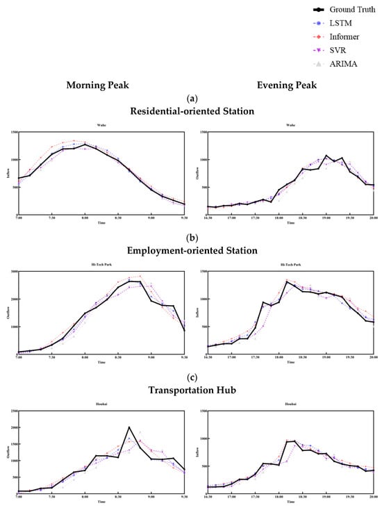
Figure 9.
Visualization of the forecast results of three types of typical stations during peak hours. (a) Wuhe station. (b) Hi-Tech Park station. (c) Houhai station.
Here are some key considerations that might explain why LSTM outperformed informer in our metro passenger flow prediction task.
- LSTMs are excellent at capturing local temporal patterns and short-term dependencies, which might be prevalent in our metro passenger flow data. Transformers are powerful in capturing long-range dependencies and complex patterns, which might be more useful in datasets with longer historical dependencies or more complex temporal interactions.
- LSTMs tend to perform well with smaller datasets. They can overfit less easily than transformers if the data are limited. Transformers generally require larger datasets to train effectively. They are data hungry and might not perform as well with smaller datasets due to their large number of parameters and high complexity.
- LSTMs can sometimes handle noisy data better due to their gating mechanisms that control the flow of information. Transformers can be sensitive to noise, and their performance might degrade if the data are not clean or highly variable without sufficient training data to generalize well.
- LSTMs have a simpler architecture compared to transformers, which might make them easier to train and tune, especially when computational resources are limited. Transformers, with their self-attention mechanisms and multi-head attention, are more complex and require more computational resources for training. This complexity can be a disadvantage if the computational infrastructure is not robust enough.
- For tasks with clear and strong temporal dependencies, LSTMs can effectively leverage their ability to remember previous states. Transformers can provide better performance for tasks that benefit from capturing broader contextual information and where interactions are not strictly sequential.
Additionally, it is noteworthy that Sun et al. proposed a novel type of RNN layer termed TTT, which exhibits linear complexity and a highly expressive hidden state. This model employs the hidden state as a machine learning model, where the update rule is derived from self-supervised learning steps. This innovation enables updating the hidden state during test sequences to equate to model training at test time. The TTT layer lowers perplexity by conditioning on more tokens in extended contexts, thereby demonstrating superior performance compared to transformers. Additionally, the TTT-RNN introduces advances in hardware efficiency and system optimization, revealing significant potential for processing long contexts. Such innovations provide promising avenues for future applications in traffic prediction utilizing RNNs.
In summary, while transformers generally excel in tasks involving longer sequences and more complex temporal patterns, LSTMs might outperform in situations where the data have shorter sequences, stronger local temporal dependencies, and a relatively small dataset size. The specific characteristics of our metro passenger flow data likely favored the strengths of LSTMs, leading to their better performance in the short-term metro passenger flow prediction task. Therefore, selecting an appropriate model that considers the dataset and computational resources is crucial for traffic prediction tasks. Sometimes, simpler models can provide more accurate and efficient predictions in certain prediction tasks.
6.2. Discussion: RNNs vs. Other Prediction Models
With the increasing popularity, we first discuss the comparison between RNNs and statistical models, focusing on the comparison between RNNs and the representative work of statistical learning models, ARIMA. The ARIMA model is relatively simple, easy to understand and implement, and has low requirements for data preprocessing. Initially, ARIMA models were used for short-term traffic flow predictions, often restricted to a single arterial roadway or a small subset of an urban network. ARIMA models can provide reliable predictions in scenarios where the data are stable and the linear relationship is apparent. However, there are significant drawbacks, especially when dealing with complex, non-stationary time series data. ARIMA models typically assume that the data are stationary, which limits their ability to predict traffic during more complicated conditions, like peak traffic periods. Their ability to handle non-stationary data is limited. Although non-stationarity can be addressed through methods, such as differencing, traditional statistical models, typically do not perform as well as deep learning models when dealing with non-stationary data with complex seasonal and trend patterns. Liu et al. [140] evaluated the performance of LSTMs against statistical learning models in traffic flow prediction. The study indicates that integrating LSTMs with other neural network architectures shows better predictive results than ARIMA. Compared to the ARIMA model, LSTMs are more suitable for complex and dynamic traffic flow predictions, enabling better capture of key traffic flow characteristics. This is mainly attributed to LSTM’s ability to model data with non-stationary patterns without pre-differencing or transformations effectively. Additionally, the structure of LSTMs allows them to learn from relatively complex data patterns, which is advantageous when dealing with the multidimensional nature of traffic systems, including spatial interactions and temporal dynamics. It is worth mentioning that RNNs and their variants naturally support multivariate input, making it easy to handle traffic data from multiple sites or road segments. In contrast, the ARIMA model is designed for univariate time series, dealing with autoregression, differencing, and moving averages of a single time series. Therefore, the ARIMA model used to forecast traffic flow predicts the flow for a single measurement point or road segment. In comparison, RNNs and their variants, like LSTMs and GRUs, can naturally handle inputs from multiple data sources and effectively capture the temporal dependencies and interaction effects among these variables. This makes them perform better in applications, such as traffic flow prediction, where analyzing and forecasting dynamic interactions across multiple points are required.
Next, we discuss the comparison between RNNs and traditional machine learning models. Firstly, regarding handling time series data, K-NN and SVR are not specifically designed for sequence prediction. They often require complex feature engineering to include time information, such as creating time window features or lag features. While these models perform well on non-time series data, like classification and regression problems, they are less intuitive or efficient than RNNs in native time series processing. When dealing with multivariate and spatial relationships, RNNs support multivariate input, enabling the simultaneous prediction of data from multiple traffic monitoring points. Although RNNs do not directly handle spatial data, incorporating techniques, like CNN layers or attention mechanisms, allows for effective learning of spatial relationships between points in the traffic network. In traditional machine learning, models like K-NN and SVR can handle multivariate problems but often lack built-in mechanisms for handling spatial or temporal dependencies. They are not very efficient when dealing with data from multiple monitoring points. Additionally, these models do not inherently incorporate mechanisms for analyzing spatial relationships and require complex data preprocessing or feature engineering to include this information indirectly. Considering the aspect of model interpretability, traditional machine learning models have relatively simple algorithms and fewer parameters, making their decision processes easy to understand. The outputs of these models are easily interpretable, aiding in the analysis and validation of prediction results’ reasonableness. In contrast, RNNs are less intuitive compared to traditional machine learning models.
As shown in Table 4, the experimental results using the AFC dataset reveal that the prediction performance of the ARIMA model, representing statistical learning models, and the SVR model, representing traditional machine learning, do not have an advantage over RNNs.
Finally, we discuss TCN models, which have shown excellent performance in time series forecasting compared to RNNs and their variants and other deep learning models. Earlier, we outlined the fundamental characteristics of these two types of models. Given that TCN’s development occurs later than RNNs, we now discuss the specific features of TCNs in the context of traffic prediction compared to RNNs. Firstly, TCN’s advantage lies in its parallel processing capability. In contrast to RNNs, where predicting the next time step requires waiting for the computation of the previous step to complete, TCNs can process the entire sequence in parallel. This makes TCNs more efficient in handling long-time series traffic data, enabling quick responses to changes in traffic flow and making it suitable for real-time or near-real-time traffic prediction systems. TCNs can also flexibly adjust their receptive field by tuning the number of dilated convolution layers, dilation factors, or filter sizes, allowing them to adapt to different lengths of historical data. Different traffic scenarios require varying lengths of historical data for effective prediction. Regarding gradient stability, TCNs avoid the problem of exploding or vanishing gradients compared to RNNs. This is because TCN’s backpropagation is independent of the time direction. This characteristic enhances the stability of model training, which is particularly crucial for traffic data scenarios that often involve sudden events and non-linear changes. Additionally, when handling long input sequences, TCNs are more efficient than RNNs and their variants, like LSTM and GRUs. This efficiency stems from TCN’s shared filters across layers, where the complexity of backpropagation is mainly determined by the network depth, making it feasible to handle large-scale traffic data in resource-constrained environments. In terms of inputting traffic data, TCNs and RNNs can handle input sequences of arbitrary lengths, allowing flexibility in dealing with different situations in traffic data. However, TCNs have some notable drawbacks. For instance, during the testing phase, TCNs require storing sufficient historical data to generate predictions. In contrast, RNNs only need to maintain hidden states and receive the current input to create predictions. Consequently, TCNs may require more memory during testing. Moreover, when transitioning from an application scenario with lower historical data requirements to one with greater historical data demands, TCNs may need to increase their receptive field size to adapt to the new requirements. This may entail significant adjustments to the model architecture, increasing the complexity of model tuning.
6.3. Challenges and Future Directions
6.3.1. Improve Model Interpretability
Improving the interpretability of RNNs in traffic prediction is not only a technical requirement to enhance model transparency but also a key factor in achieving efficient traffic management and precise decision support. Interpretable models enable traffic managers and decision makers to understand the logic and influencing factors behind model predictions. For example, suppose a traffic prediction model can clearly show the reasons for traffic congestion during a certain period (such as weekday rush hours, holidays, or special events). In that case, decision makers can adjust traffic signal control or implement traffic control measures based on these insights. Additionally, when the model can provide easily understandable prediction processes and results, the trustworthiness of these predictions increases among the public and policymakers. This is crucial for promoting the application of intelligent transportation systems and the acceptance of new technologies. On the other hand, by enhancing the interpretability of models, developers can more easily identify biases in the data or algorithms, such as geographic biases or systematic biases in data collection, thereby improving the fairness and accuracy of the model. Improving models’ interpretability is crucial for developing deep learning models in traffic prediction. However, enhancing the interpretability of deep learning models and further exploring their superiority and rationality remains a significant challenge.
In future research, enhancing model interpretability can be pursued through two main directions. On the one hand, improvements can be made from within the model itself, such as simplifying model architectures and integrating interpretability mechanisms to ensure that while the model achieves high-performance traffic prediction, it maintains a transparent and explainable decision-making structure. On the other hand, developing visualization tools to represent the predictive model’s internal workings and decision processes can reveal the underlying logic behind the model’s predictions, thereby improving its interpretability.
6.3.2. Long-Term Dependencies of Traffic Data in Short-Term Traffic Prediction
Long-term dependencies in traffic data are patterns and trends that extend over a significant time span and influence short-term traffic conditions. By incorporating these dependencies, short-term traffic prediction models can more accurately forecast immediate traffic conditions by considering historical data and broader temporal patterns. When using RNNs for extracting long-term dependencies of traffic data in short-term prediction, issues such as vanishing or exploding gradients often lead to training difficulties. This is because, during backpropagation, gradients can quickly diminish or grow exponentially with each layer, especially when dealing with long sequences. Additionally, capturing long-term dependencies is challenging with RNNs due to the difficulty in capturing long-term dependencies. In long sequences, the current output may depend on inputs from a long time ago, and due to the vanishing gradient problem, these long-term dependencies cannot be effectively learned through backpropagation through time. The network struggles to understand these critical historical dependencies, leading to decreased prediction performance. This limits the model’s ability to predict over long periods, while the information contained in long time series is crucial for predicting future traffic conditions. As the prediction period increases, effectively utilizing historical long-term data to maintain prediction accuracy becomes a major challenge.
In future research, further investigation and development of innovative deep learning architectures will be crucial for addressing long-term dependency issues. For instance, novel RNN layers, such as TTT [1], employ new model designs to compress and represent inputs, dynamically adjusting the internal structure of the model to accommodate input data and capture long-term dependencies. Such innovative approaches offer promising directions for better capturing and utilizing long-term dependencies.
6.3.3. Lack of a Comprehensive Multi-Scenario Baseline Dataset
In the field of traffic prediction, despite the existence of high-quality datasets, such as the PeMS dataset, current data resources often focus on specific regions or types of roads (such as highways) and are not sufficient to comprehensively cover diverse traffic scenarios, such as urban streets, rural roads, or those in different countries and regions. Additionally, existing datasets often lack traffic flow data during changing weather conditions, holidays, or large events, as well as data from daily peak and off-peak periods, all of which are important factors affecting traffic flow. Effective traffic prediction models need to process multiple types of data, such as real-time location and speed information from floating car data, road network data, and exogenous data, like weather and population density. However, the lack of a unified and widely accepted baseline dataset makes it difficult to compare model performance between different studies, affecting the evaluation and validation of models.
In future research, creating a comprehensive, diverse, and widely applicable standard dataset is crucial. It can improve models’ accuracy and generalization ability, promote the reproducibility of research results, and further technological innovation.
6.3.4. Missing Data Problem
When using RNNs for traffic prediction, data integrity is crucial for model performance. Traffic data are typically collected from sensors, cameras, or GPS devices, and these data collection tools may result in data missing due to failures, communication interruptions, or processing errors. These missing data can decrease model training and prediction accuracy, as RNNs rely on complete time series data to learn the dynamic changes in traffic flow.
In future research, to address the issue of missing data, researchers need to develop and apply effective data imputation techniques, such as estimating missing values using historical data trends or employing machine learning methods to fill in missing data automatically. However, ensuring the accuracy and reliability of data imputation methods remains a challenge. Additionally, solutions can be found through techniques such as few-shot learning or transfer learning. Few-shot learning aims to enable models to quickly learn and adapt to new tasks with a small amount of data and is particularly useful in scenarios with scarce data. By pre-training models on large datasets to learn general feature representations and then transferring this knowledge to specific traffic prediction tasks, accuracy can be improved in cases of limited data availability. Furthermore, data augmentation techniques are also a strategy to address missing data, as they can increase the diversity of training samples and reduce the risk of overfitting.
6.3.5. Processing Multi-Source Heterogeneous Data
Traffic prediction involves a variety of data sources, including road sensors, vehicle sensors, video surveillance, GPS devices, social media, and meteorological stations, all of which are large in scale and diverse in form. Initially, these different data sources provide various formats of data; for instance, sensors typically offer real-time traffic flow figures, video surveillance yields image data, and GPS devices provide geographical location and timestamp information. Furthermore, the accuracy and update frequency of data from these sources vary; GPS data may update multiple times per second, while some sensors update less frequently. Additionally, due to potential asynchrony in device clocks, there may be slight discrepancies in the time stamps of data from different sources. Lastly, data may be missing due to various reasons, such as equipment failure or communication disruptions. Facing the massive multi-source heterogeneous data, how to build a suitable deep learning model that can fully tap the value of these data for traffic prediction will become a major challenge in the future.
Therefore, future development needs to focus on extracting useful features from these data sources and using ensemble learning methods or multi-model fusion techniques to combine the predictive results from these sources, thereby enhancing the accuracy and robustness of predictions. Moreover, developing more intelligent data fusion algorithms that automatically identify and utilize information from each data source is key to improving data utilization and enhancing the adaptive capacity of predictions.
7. Conclusions
This paper provided a comprehensive review of the application of RNNs in traffic prediction. Specifically, we first outlined the history of traffic prediction, classified existing traffic prediction methods based on existing input sequence representation methods and forms, and summarized in detail the research progress on predicting tasks with different input sequence lengths. The discussion on input data representation emphasized the importance of choosing appropriate data formats to optimize model performance. Additionally, we summarized the classical models, RNNs, and their variants, as well as hybrid models combined with RNNs applied to traffic prediction. Next, we presented the representative results for seven traffic prediction tasks, providing a comprehensive overview of research progress in different application scenarios. Finally, we discussed the comparison between RNNs and popular deep learning models and the major challenges.
The key findings of our review are listed as follows:
- RNNs are extensively utilized in traffic prediction. In processing various types of traffic data, RNNs not only efficiently handle time series data independently but also serve as temporal feature extraction modules when combined with models, such as CNNs and GNNs, for spatiotemporal data processing. Furthermore, RNNs play a significant role across seven sub-areas within traffic prediction.
- RNNs are expected to continue being preferred models for future traffic prediction tasks due to their advantages and will not be replaced by transformers. We conducted a comparative study using real-world metro smart card datasets for short-term passenger flow prediction. This allowed us to directly compare the predictive performance of RNNs (particularly LSTMs) with other models in a real and specific environment. The results showed that, despite the presence of more advanced transformer models, RNNs demonstrated superior performance. This finding underscores the importance of selecting the appropriate model based on the characteristics of different datasets and available resources, as sometimes simpler models can provide more accurate and efficient predictions.
This paper served as a valuable resource for participants seeking a comprehensive understanding of traffic prediction, enabling them to identify areas of interest quickly. It offered a thorough reference for researchers, facilitating exploration and fostering the advancement of related studies in the field. By providing an in-depth analysis of the application of RNNs in traffic prediction, this review aimed to promote innovation and development, encouraging the design of more effective traffic prediction models and integrating advanced methodologies. Ultimately, it aspired to contribute to the progress and refinement of traffic prediction research, benefiting theoretical exploration and practical application.
Author Contributions
Conceptualization, Y.H. and K.-L.T.; methodology, Y.H. and P.H.; software, W.H.; validation, Y.H., P.H. and W.H.; formal analysis, P.H.; investigation, P.H.; resources, Y.H. and Q.L.; data curation, Y.H. and W.H.; writing—original draft preparation, Y.H. and P.H.; writing—review and editing, Y.H., L.L. and K.-L.T.; visualization, P.H. and W.H.; supervision, K.-L.T.; project administration, Y.H.; funding acquisition, Y.H. and Q.L. All authors have read and agreed to the published version of the manuscript.
Funding
This study was supported by the National Natural Science Foundation of China (72301180); the Guangdong Basic and Applied Basic Research Foundation (2021A1515110731); the Shenzhen Science and Technology Program (RCBS20231211090512002); the Shanghai Key Laboratory of Rail Infrastructure Durability and System Safety (R202203); Natural Science Foundation of Top Talent of SZTU (GDRC202126); a grant from the Department of Education of Guangdong Province (2022KCXTD027); and the Guangdong Key Construction Discipline Research Ability Enhancement Project (2021ZDJS108).
Conflicts of Interest
The authors declare no conflict of interest.
References
- Sun, Y.; Li, X.; Dalal, K.; Xu, J.; Vikram, A.; Zhang, G.; Dubois, Y.; Chen, X.; Wang, X.; Koyejo, S. Learning to (Learn at Test Time): RNNs with Expressive Hidden States. arXiv 2024, arXiv:2407.04620. [Google Scholar]
- Beck, M.; Pöppel, K.; Spanring, M.; Auer, A.; Prudnikova, O.; Kopp, M.; Klambauer, G.; Brandstetter, J.; Hochreiter, S. xLSTM: Extended Long Short-Term Memory. arXiv 2024, arXiv:2405.04517. [Google Scholar]
- Smith, B.L.; Demetsky, M.J. Traffic flow forecasting: Comparison of modeling approaches. J. Transp. Eng. 1997, 123, 261–266. [Google Scholar] [CrossRef]
- Gardner, E.S., Jr. Exponential smoothing: The state of the art. J. Forecast. 1985, 4, 1–28. [Google Scholar] [CrossRef]
- Hamed, M.M.; Al-Masaeid, H.R.; Said, Z.M.B. Short-term prediction of traffic volume in urban arterials. J. Transp. Eng. 1995, 121, 249–254. [Google Scholar] [CrossRef]
- Kamarianakis, Y.; Prastacos, P. Space–time modeling of traffic flow. Comput. Geosci. 2005, 31, 119–133. [Google Scholar] [CrossRef]
- Li, X.; Pan, G.; Wu, Z.; Qi, G.; Li, S.; Zhang, D.; Zhang, W.; Wang, Z. Prediction of urban human mobility using large-scale taxi traces and its applications. Front. Comput. Sci. 2012, 6, 111–121. [Google Scholar] [CrossRef]
- Moreira-Matias, L.; Gama, J.; Ferreira, M.; Mendes-Moreira, J.; Damas, L. Predicting taxi–passenger demand using streaming data. IEEE Trans. Intell. Transp. Syst. 2013, 14, 1393–1402. [Google Scholar] [CrossRef]
- Lippi, M.; Bertini, M.; Frasconi, P. Short-term traffic flow forecasting: An experimental comparison of time-series analysis and supervised learning. IEEE Trans. Intell. Transp. Syst. 2013, 14, 871–882. [Google Scholar] [CrossRef]
- Wagner-Muns, I.M.; Guardiola, I.G.; Samaranayke, V.; Kayani, W.I. A functional data analysis approach to traffic volume forecasting. IEEE Trans. Intell. Transp. Syst. 2017, 19, 878–888. [Google Scholar] [CrossRef]
- Wang, H.; Zhang, B. Research on ARIMA Model for Short-Term Traffic Flow Prediction based on Time Series. In Proceedings of the 2023 8th International Conference on Intelligent Informatics and Biomedical Sciences (ICIIBMS), Okinawa, Japan, 23–25 November 2023; pp. 92–95. [Google Scholar]
- Ahmed, M.S.; Cook, A.R. Analysis of Freeway Traffic Time-Series Data by Using Box-Jenkins Techniques; Transportation Research Board: Washington, DC, USA, 1979. [Google Scholar]
- Williams, B.M.; Hoel, L.A. Modeling and forecasting vehicular traffic flow as a seasonal ARIMA process: Theoretical basis and empirical results. J. Transp. Eng. 2003, 129, 664–672. [Google Scholar] [CrossRef]
- Guan, J.; Wang, W.; Li, W.; Zhou, S. A unified framework for predicting kpis of on-demand transport services. IEEE Access 2018, 6, 32005–32014. [Google Scholar] [CrossRef]
- Zheng, L.; Zhu, C.; Zhu, N.; He, T.; Dong, N.; Huang, H. Feature selection-based approach for urban short-term travel speed prediction. IET Intell. Transp. Syst. 2018, 12, 474–484. [Google Scholar] [CrossRef]
- Diao, Z.; Zhang, D.; Wang, X.; Xie, K.; He, S.; Lu, X.; Li, Y. A hybrid model for short-term traffic volume prediction in massive transportation systems. IEEE Trans. Intell. Transp. Syst. 2018, 20, 935–946. [Google Scholar] [CrossRef]
- Salinas, D.; Bohlke-Schneider, M.; Callot, L.; Medico, R.; Gasthaus, J. High-dimensional multivariate forecasting with low-rank gaussian copula processes. In Proceedings of the Advances in Neural Information Processing Systems 32: Annual Conference on Neural Information Processing Systems, NeurIPS 2019, Vancouver, BC, Canada, 8–14 December 2019. [Google Scholar]
- Sun, S.; Xu, X. Variational inference for infinite mixtures of Gaussian processes with applications to traffic flow prediction. IEEE Trans. Intell. Transp. Syst. 2010, 12, 466–475. [Google Scholar] [CrossRef]
- Zhao, J.; Sun, S. High-order Gaussian process dynamical models for traffic flow prediction. IEEE Trans. Intell. Transp. Syst. 2016, 17, 2014–2019. [Google Scholar] [CrossRef]
- Gong, Y.; Li, Z.; Zhang, J.; Liu, W.; Zheng, Y.; Kirsch, C. Network-wide crowd flow prediction of sydney trains via customized online non-negative matrix factorization. In Proceedings of the 27th ACM International Conference on Information and Knowledge Management, Torino, Italy, 22–26 October 2018; pp. 1243–1252. [Google Scholar]
- Shin, J.; Sunwoo, M. Vehicle speed prediction using a Markov chain with speed constraints. IEEE Trans. Intell. Transp. Syst. 2018, 20, 3201–3211. [Google Scholar] [CrossRef]
- Zhu, G.; Song, K.; Zhang, P.; Wang, L. A traffic flow state transition model for urban road network based on Hidden Markov Model. Neurocomputing 2016, 214, 567–574. [Google Scholar] [CrossRef]
- Shahi, T.B.; Shrestha, A.; Neupane, A.; Guo, W. Stock price forecasting with deep learning: A comparative study. Mathematics 2020, 8, 1441. [Google Scholar] [CrossRef]
- Shahi, T.B.; Sitaula, C. Natural language processing for Nepali text: A review. Artif. Intell. Rev. 2022, 55, 3401–3429. [Google Scholar] [CrossRef]
- Innamaa, S. Short-term prediction of traffic situation using MLP-neural networks. In Proceedings of the 7th World Congress on Intelligent Transport Systems, Turin, Italy, 6–9 November 2000; pp. 6–9. [Google Scholar]
- Taylor, C.; Meldrum, D. Freeway traffic data prediction using neural networks. In Proceedings of the Pacific Rim TransTech Conference. 1995 Vehicle Navigation and Information Systems Conference Proceedings. 6th International VNIS. A Ride into the Future, Seattle, WA, USA, 30 July–2 August 1995; pp. 225–230. [Google Scholar]
- Ledoux, C. An urban traffic flow model integrating neural networks. Transp. Res. Part C Emerg. Technol. 1997, 5, 287–300. [Google Scholar] [CrossRef]
- Ma, X.; Tao, Z.; Wang, Y.; Yu, H.; Wang, Y. Long short-term memory neural network for traffic speed prediction using remote microwave sensor data. Transp. Res. Part C Emerg. Technol. 2015, 54, 187–197. [Google Scholar] [CrossRef]
- Tian, Y.; Pan, L. Predicting short-term traffic flow by long short-term memory recurrent neural network. In Proceedings of the 2015 IEEE International Conference on Smart City/SocialCom/SustainCom (SmartCity), Chengdu, China, 19–21 December 2015; pp. 153–158. [Google Scholar]
- Fu, R.; Zhang, Z.; Li, L. Using LSTM and GRU neural network methods for traffic flow prediction. In Proceedings of the 2016 31st Youth Academic Annual Conference of Chinese Association of Automation (YAC), Wuhan, China, 11–13 November 2016; pp. 324–328. [Google Scholar]
- Liu, Y.; Zheng, H.; Feng, X.; Chen, Z. Short-term traffic flow prediction with Conv-LSTM. In Proceedings of the 2017 9th International Conference on Wireless Communications and Signal Processing (WCSP), Nanjing, China, 11–13 October 2017; pp. 1–6. [Google Scholar]
- Zhao, Z.; Chen, W.; Wu, X.; Chen, P.C.; Liu, J. LSTM network: A deep learning approach for short-term traffic forecast. IET Intell. Transp. Syst. 2017, 11, 68–75. [Google Scholar] [CrossRef]
- Ma, X.; Dai, Z.; He, Z.; Ma, J.; Wang, Y.; Wang, Y. Learning traffic as images: A deep convolutional neural network for large-scale transportation network speed prediction. Sensors 2017, 17, 818. [Google Scholar] [CrossRef]
- Song, C.; Lee, H.; Kang, C.; Lee, W.; Kim, Y.B.; Cha, S.W. Traffic speed prediction under weekday using convolutional neural networks concepts. In Proceedings of the 2017 IEEE Intelligent Vehicles Symposium (IV), Los Angeles, CA, USA, 11–14 June 2017; pp. 1293–1298. [Google Scholar]
- Lea, C.; Vidal, R.; Reiter, A.; Hager, G.D. Temporal convolutional networks: A unified approach to action segmentation. In Proceedings of the Computer Vision–ECCV 2016 Workshops, Amsterdam, The Netherlands, 8–10 and 15–16 October 2016; Proceedings, Part III 14. pp. 47–54. [Google Scholar]
- Zhao, W.; Gao, Y.; Ji, T.; Wan, X.; Ye, F.; Bai, G. Deep temporal convolutional networks for short-term traffic flow forecasting. IEEE Access 2019, 7, 114496–114507. [Google Scholar] [CrossRef]
- Bi, J.; Zhang, X.; Yuan, H.; Zhang, J.; Zhou, M. A hybrid prediction method for realistic network traffic with temporal convolutional network and LSTM. IEEE Trans. Autom. Sci. Eng. 2021, 19, 1869–1879. [Google Scholar] [CrossRef]
- Ren, Y.; Zhao, D.; Luo, D.; Ma, H.; Duan, P. Global-local temporal convolutional network for traffic flow prediction. IEEE Trans. Intell. Transp. Syst. 2020, 23, 1578–1584. [Google Scholar] [CrossRef]
- Li, Y.; Yu, R.; Shahabi, C.; Liu, Y. Diffusion convolutional recurrent neural network: Data-driven traffic forecasting. arXiv 2017, arXiv:1707.01926. [Google Scholar]
- Yu, B.; Yin, H.; Zhu, Z. Spatio-temporal graph convolutional networks: A deep learning framework for traffic forecasting. arXiv 2017, arXiv:1709.04875. [Google Scholar]
- Guo, S.; Lin, Y.; Feng, N.; Song, C.; Wan, H. Attention based spatial-temporal graph convolutional networks for traffic flow forecasting. In Proceedings of the AAAI Conference on Artificial Intelligence, Honolulu, HI, USA, 27 January–1 February 2019; pp. 922–929. [Google Scholar]
- Zhao, L.; Song, Y.; Zhang, C.; Liu, Y.; Wang, P.; Lin, T.; Deng, M.; Li, H. T-gcn: A temporal graph convolutional network for traffic prediction. IEEE Trans. Intell. Transp. Syst. 2019, 21, 3848–3858. [Google Scholar] [CrossRef]
- Wu, Z.; Pan, S.; Long, G.; Jiang, J.; Zhang, C. Graph wavenet for deep spatial-temporal graph modeling. arXiv 2019, arXiv:1906.00121. [Google Scholar]
- Lv, M.; Hong, Z.; Chen, L.; Chen, T.; Zhu, T.; Ji, S. Temporal multi-graph convolutional network for traffic flow prediction. IEEE Trans. Intell. Transp. Syst. 2020, 22, 3337–3348. [Google Scholar] [CrossRef]
- Lan, S.; Ma, Y.; Huang, W.; Wang, W.; Yang, H.; Li, P. Dstagnn: Dynamic spatial-temporal aware graph neural network for traffic flow forecasting. In Proceedings of the International Conference on Machine Learning, Baltimore, MD, USA, 17–23 July 2022; pp. 11906–11917. [Google Scholar]
- Ashish, V. Attention is all you need. Adv. Neural Inf. Process. Syst. 2017, 30, 1. [Google Scholar]
- Cai, L.; Janowicz, K.; Mai, G.; Yan, B.; Zhu, R. Traffic transformer: Capturing the continuity and periodicity of time series for traffic forecasting. Trans. GIS 2020, 24, 736–755. [Google Scholar] [CrossRef]
- Zhou, H.; Zhang, S.; Peng, J.; Zhang, S.; Li, J.; Xiong, H.; Zhang, W. Informer: Beyond efficient transformer for long sequence time-series forecasting. In Proceedings of the AAAI Conference on Artificial Intelligence, Virtual, 2–9 February 2021; pp. 11106–11115. [Google Scholar]
- Jiang, J.; Han, C.; Zhao, W.X.; Wang, J. Pdformer: Propagation delay-aware dynamic long-range transformer for traffic flow prediction. In Proceedings of the AAAI Conference on Artificial Intelligence, Washington, DC, USA, 7–14 February 2023; pp. 4365–4373. [Google Scholar]
- Rawat, D.; Singh, V.; Dhondiyal, S.A.; Singh, S. Time Series Forecasting Models: A Comprehensive. Available online: https://www.researchgate.net/publication/373439013_Time_Series_Forecasting_Models_A_Comprehensive_Review (accessed on 4 September 2024).
- Tokuyama, Y.; Fukushima, Y.; Yokohira, T. The effect of using attribute information in network traffic prediction with deep learning. In Proceedings of the 2018 International Conference on Information and Communication Technology Convergence (ICTC), Jeju Island, Republic of Korea, 17–19 October 2018; pp. 521–525. [Google Scholar]
- Qu, L.; Lyu, J.; Li, W.; Ma, D.; Fan, H. Features injected recurrent neural networks for short-term traffic speed prediction. Neurocomputing 2021, 451, 290–304. [Google Scholar] [CrossRef]
- Wang, X.; Xu, L.; Chen, K. Data-driven short-term forecasting for urban road network traffic based on data processing and LSTM-RNN. Arab. J. Sci. Eng. 2019, 44, 3043–3060. [Google Scholar]
- Awan, F.M.; Minerva, R.; Crespi, N. Using noise pollution data for traffic prediction in smart cities: Experiments based on LSTM recurrent neural networks. IEEE Sens. J. 2021, 21, 20722–20729. [Google Scholar] [CrossRef]
- Zhang, J.; Zheng, Y.; Qi, D. Deep spatio-temporal residual networks for citywide crowd flows prediction. In Proceedings of the AAAI Conference on Artificial Intelligence, San Francisco, CA, USA, 4–9 February 2017. [Google Scholar]
- Yao, H.; Wu, F.; Ke, J.; Tang, X.; Jia, Y.; Lu, S.; Gong, P.; Ye, J.; Li, Z. Deep multi-view spatial-temporal network for taxi demand prediction. In Proceedings of the AAAI Conference on Artificial Intelligence, New Orleans, LO, USA, 2–7 February 2018. [Google Scholar]
- Bao, J.; Yu, H.; Wu, J. Short-term FFBS demand prediction with multi-source data in a hybrid deep learning framework. IET Intell. Transp. Syst. 2019, 13, 1340–1347. [Google Scholar] [CrossRef]
- Zhou, X.; Shen, Y.; Zhu, Y.; Huang, L. Predicting multi-step citywide passenger demands using attention-based neural networks. In Proceedings of the Eleventh ACM International Conference on Web Search and Data Mining, Marina Del Rey, CA, USA, 5–9 February 2018; pp. 736–744. [Google Scholar]
- Roudbari, N.S.; Patterson, Z.; Eicker, U.; Poullis, C. Simpler is better: Multilevel abstraction with graph convolutional recurrent neural network cells for traffic prediction. In Proceedings of the 2022 IEEE Symposium Series on Computational Intelligence (SSCI), Singapore, 4–7 December 2022; pp. 1–10. [Google Scholar]
- Lu, Z.; Lv, W.; Cao, Y.; Xie, Z.; Peng, H.; Du, B. LSTM variants meet graph neural networks for road speed prediction. Neurocomputing 2020, 400, 34–45. [Google Scholar] [CrossRef]
- Wang, H.; Zhang, R.; Cheng, X.; Yang, L. Hierarchical traffic flow prediction based on spatial-temporal graph convolutional network. IEEE Trans. Intell. Transp. Syst. 2022, 23, 16137–16147. [Google Scholar] [CrossRef]
- James, J. Graph construction for traffic prediction: A data-driven approach. IEEE Trans. Intell. Transp. Syst. 2022, 23, 15015–15027. [Google Scholar]
- Gu, Y.; Deng, L. Stagcn: Spatial–temporal attention graph convolution network for traffic forecasting. Mathematics 2022, 10, 1599. [Google Scholar] [CrossRef]
- Sugiartawan, P.; Hartati, S. Time series data prediction using elman recurrent neural network on tourist visits in tanah lot tourism object. J. Sist. Inf. Dan Komput. Terap. Indones 2019, 1, 314–320. [Google Scholar] [CrossRef]
- Hussain, B.; Afzal, M.K.; Ahmad, S.; Mostafa, A.M. Intelligent traffic flow prediction using optimized GRU model. IEEE Access 2021, 9, 100736–100746. [Google Scholar] [CrossRef]
- Lu, S.; Zhang, Q.; Chen, G.; Seng, D. A combined method for short-term traffic flow prediction based on recurrent neural network. Alex. Eng. J. 2021, 60, 87–94. [Google Scholar] [CrossRef]
- Kashyap, A.A.; Raviraj, S.; Devarakonda, A.; Nayak, K.S.R.; Santhosh, K.V.; Bhat, S.J. Traffic flow prediction models—A review of deep learning techniques. Cogent Eng. 2022, 9, 2010510. [Google Scholar] [CrossRef]
- Chung, J.; Gulcehre, C.; Cho, K.; Bengio, Y. Gated feedback recurrent neural networks. In Proceedings of the International Conference on Machine Learning, Lille, France, 6–11 July 2015; pp. 2067–2075. [Google Scholar]
- Luo, X.; Li, D.; Yang, Y.; Zhang, S. Spatiotemporal traffic flow prediction with KNN and LSTM. J. Adv. Transp. 2019, 2019, 4145353. [Google Scholar] [CrossRef]
- Zhou, L.; Zhang, Q.; Yin, C.; Ye, W. Research on Short-term Traffic Flow Prediction Based on KNN-GRU. In Proceedings of the 2022 China Automation Congress (CAC), Xiamen, China, 25–27 November 2022; pp. 1924–1928. [Google Scholar]
- Tong, J.; Gu, X.; Zhang, M.; Wan, J.; Wang, J. Traffic flow prediction based on improved SVR for VANET. In Proceedings of the 2021 4th International Conference on Advanced Electronic Materials, Computers and Software Engineering (AEMCSE), Changsha, China, 26–28 March 2021; pp. 402–405. [Google Scholar]
- Cai, L.; Chen, Q.; Cai, W.; Xu, X.; Zhou, T.; Qin, J. SVRGSA: A hybrid learning based model for short-term traffic flow forecasting. IET Intell. Transp. Syst. 2019, 13, 1348–1355. [Google Scholar] [CrossRef]
- Yu, H.; Wu, Z.; Wang, S.; Wang, Y.; Ma, X. Spatiotemporal recurrent convolutional networks for traffic prediction in transportation networks. Sensors 2017, 17, 1501. [Google Scholar] [CrossRef]
- Yao, H.; Tang, X.; Wei, H.; Zheng, G.; Li, Z. Revisiting spatial-temporal similarity: A deep learning framework for traffic prediction. In Proceedings of the AAAI Conference on Artificial Intelligence, Honolulu, HI, USA, 27 January–1 February 2019; pp. 5668–5675. [Google Scholar]
- Wang, X.; Ma, Y.; Wang, Y.; Jin, W.; Wang, X.; Tang, J.; Jia, C.; Yu, J. Traffic flow prediction via spatial temporal graph neural network. In Proceedings of the Web Conference, Taipei, Taiwan, 20–24 April 2020; pp. 1082–1092. [Google Scholar]
- Bogaerts, T.; Masegosa, A.D.; Angarita-Zapata, J.S.; Onieva, E.; Hellinckx, P. A graph CNN-LSTM neural network for short and long-term traffic forecasting based on trajectory data. Transp. Res. Part C Emerg. Technol. 2020, 112, 62–77. [Google Scholar] [CrossRef]
- Qin, G.; Niu, X.; Wang, J.; Qian, Q. Traffic flow prediction based on JANet and attention mechanism. In Proceedings of the 2021 6th International Conference on Intelligent Computing and Signal Processing (ICSP), Xi’an, China, 9–11 April 2021; pp. 131–134. [Google Scholar]
- Hu, H.; Lin, Z.; Hu, Q.; Zhang, Y. Attention mechanism with spatial-temporal joint model for traffic flow speed prediction. IEEE Trans. Intell. Transp. Syst. 2021, 23, 16612–16621. [Google Scholar] [CrossRef]
- Yu, J.; Wei, H.; Guo, H.; Cai, Y. Urban traffic state prediction based on SA-LSTM. IOP Conf. Ser. Earth Environ. Sci. 2021, 783, 12153. [Google Scholar] [CrossRef]
- Zhao, W.; Zhang, S.; Wang, B.; Zhou, B. Dstgrn: Traffic flow prediction via dynamic spatio-temporal graph recurrent network. In Proceedings of the 2023 3rd International Conference on Consumer Electronics and Computer Engineering (ICCECE), Guangzhou, China, 6–8 January 2023; pp. 599–604. [Google Scholar]
- Tian, X.; Du, L.; Zhang, X.; Wu, S. Mat-wgcn: Traffic speed prediction using multi-head attention mechanism and weighted adjacency matrix. Sustainability 2023, 15, 13080. [Google Scholar] [CrossRef]
- Zheng, H.; Lin, F.; Feng, X.; Chen, Y. A hybrid deep learning model with attention-based conv-LSTM networks for short-term traffic flow prediction. IEEE Trans. Intell. Transp. Syst. 2020, 22, 6910–6920. [Google Scholar] [CrossRef]
- Shu, W.; Cai, K.; Xiong, N.N. A short-term traffic flow prediction model based on an improved gate recurrent unit neural network. IEEE Trans. Intell. Transp. Syst. 2021, 23, 16654–16665. [Google Scholar] [CrossRef]
- Chen, L.; Shao, W.; Lv, M.; Chen, W.; Zhang, Y.; Yang, C. AARGNN: An attentive attributed recurrent graph neural network for traffic flow prediction considering multiple dynamic factors. IEEE Trans. Intell. Transp. Syst. 2022, 23, 17201–17211. [Google Scholar] [CrossRef]
- Huang, X.; Jiang, Y.; Tang, J. MAPredRNN: Multi-attention predictive RNN for traffic flow prediction by dynamic spatio-temporal data fusion. Appl. Intell. 2023, 53, 19372–19383. [Google Scholar] [CrossRef]
- Liu, S.; Li, Z.; Li, H. Research on short-term traffic flow prediction model based on RNN-LSTM. IOP Conf. Ser. Mater. Sci. Eng. 2020, 806, 12017. [Google Scholar] [CrossRef]
- Sengupta, A.; Das, A.; Guler, S.I. Hybrid hidden Markov LSTM for short-term traffic flow prediction. arXiv 2023, arXiv:2307.04954. [Google Scholar]
- Wang, Z.; Han, W. Traffic Flow Prediction Based on Optimized LSTM Model. In Proceedings of the 2023 3rd International Conference on Information Communication and Software Engineering (ICICSE), Chongqing, China, 7–9 April 2023; pp. 60–65. [Google Scholar]
- Zhou, Y.; He, J.; Wu, Z. Improved LSTM model for short-term traffic flow prediction with weather consideration. In Proceedings of the Eighth International Conference on Electromechanical Control Technology and Transportation (ICECTT 2023), Hangzhou, China, 19–21 May 2023; pp. 1546–1554. [Google Scholar]
- Yang, Z.; Wang, C. Short-term traffic flow prediction based on AST-MTL-CNN-GRU. IET Intell. Transp. Syst. 2023, 17, 2205–2220. [Google Scholar] [CrossRef]
- Lin, G.; Ding, J.; Ding, S.; Huang, B.; Yin, Y.; Zhang, K.; Li, Z. Passenger Flow Prediction with Transformer: The Shenzhen Metro Case. In Proceedings of the 2021 International Conference on Big Data Analysis and Computer Science (BDACS), Kunming, China, 25–27 June 2021; pp. 97–100. [Google Scholar]
- El Maazouzi, Q.; Retbi, A.; Bennani, S. Automatisation hyperparameters tuning process for times series forecasting: Application to passenger’s flow prediction on a railway network. Int. Arch. Photogramm. Remote Sens. Spat. Inf. Sci. 2022, 48, 53–60. [Google Scholar] [CrossRef]
- Izudheen, S. Short-term passenger count prediction for metro stations using LSTM network. Turk. J. Comput. Math. Educ. (TURCOMAT) 2021, 12, 4026–4034. [Google Scholar]
- Wen, X.-P. Single-site passenger flow forecast based on ga-lstm. In Proceedings of the 6th International Conference on Control Engineering and Artificial Intelligence, Virtual, 11–13 March 2022; pp. 16–20. [Google Scholar]
- Zhai, X.; Shen, Y. Short-Term Bus Passenger Flow Prediction Based on Graph Diffusion Convolutional Recurrent Neural Network. Appl. Sci. 2023, 13, 4910. [Google Scholar] [CrossRef]
- Zeng, L.; Li, Z.; Yang, J.; Xu, X. Research on short-term passenger flow prediction method of urban rail transit based on CEEMDAN-IPSO-LSTM. J. Railw. Sci. Eng. 2023, 12, 1–14. [Google Scholar]
- Xu, Z.; Hou, L.; Zhang, Y.; Zhang, J. Passenger Flow Prediction of Scenic Spot Using a GCN–RNN Model. Sustainability 2022, 14, 3295. [Google Scholar] [CrossRef]
- Wang, X.; Bai, W.; Meng, Z.; Xin, B.; Gao, R.; Lv, X. The Prediction of Flow in Railway Station Based on RRC-STGCN. IEEE Access 2023, 11, 131128–131139. [Google Scholar] [CrossRef]
- ul Islam, B.; Ahmed, S.F. Research Article Short-Term Electrical Load Demand Forecasting Based on LSTM and RNN Deep Neural Networks. Math. Probl. Eng. 2022, 2022, 2316474. [Google Scholar]
- Toqué, F.; Côme, E.; El Mahrsi, M.K.; Oukhellou, L. Forecasting dynamic public transport origin-destination matrices with long-short term memory recurrent neural networks. In Proceedings of the 2016 IEEE 19th International Conference on Intelligent Transportation Systems (ITSC), Rio de Janeiro, Brazil, 1–4 November 2016; pp. 1071–1076. [Google Scholar]
- Nejadettehad, A.; Mahini, H.; Bahrak, B. Short-term demand forecasting for online car-hailing services using recurrent neural networks. Appl. Artif. Intell. 2020, 34, 674–689. [Google Scholar] [CrossRef]
- Feng, S.; Ke, J.; Yang, H.; Ye, J. A multi-task matrix factorized graph neural network for co-prediction of zone-based and OD-based ride-hailing demand. IEEE Trans. Intell. Transp. Syst. 2021, 23, 5704–5716. [Google Scholar] [CrossRef]
- Wang, N.; Zheng, L.; Shen, H.; Li, S. Ride-hailing origin-destination demand prediction with spatiotemporal information fusion. Transp. Saf. Environ. 2024, 6, tdad026. [Google Scholar] [CrossRef]
- Gu, M.; Duan, Z.; Daily, O.D. Demand Prediction in Urban Metro Transit System: A Convolutional LSTM Neural Network with Multi-factor Fusion Channel-wise Attention. In Proceedings of the 2022 IEEE 25th International Conference on Intelligent Transportation Systems (ITSC), Macau, China, 8–12 October 2022; pp. 3398–3404. [Google Scholar]
- Kim, Y.; Wang, P.; Mihaylova, L. Structural recurrent neural network for traffic speed prediction. In Proceedings of the ICASSP 2019—2019 IEEE International Conference on Acoustics, Speech and Signal Processing (ICASSP), Brighton, UK, 12–17 May 2019; pp. 5207–5211. [Google Scholar]
- Cui, Z.; Ke, R.; Pu, Z.; Wang, Y. Deep bidirectional and unidirectional LSTM recurrent neural network for network-wide traffic speed prediction. arXiv 2018, arXiv:1801.02143. [Google Scholar]
- Lv, Z.; Xu, J.; Zheng, K.; Yin, H.; Zhao, P.; Zhou, X. Lc-rnn: A deep learning model for traffic speed prediction. In Proceedings of the IJCAI, 2018 International Joint Conference on Artificial Intelligence, Stockholm, Sweden, 13–19 July 2018; p. 27. [Google Scholar]
- Ma, C.; Zhao, Y.; Dai, G.; Xu, X.; Wong, S.-C. A novel STFSA-CNN-GRU hybrid model for short-term traffic speed prediction. IEEE Trans. Intell. Transp. Syst. 2022, 24, 3728–3737. [Google Scholar] [CrossRef]
- Abdelraouf, A.; Abdel-Aty, M.; Yuan, J. Utilizing attention-based multi-encoder-decoder neural networks for freeway traffic speed prediction. IEEE Trans. Intell. Transp. Syst. 2021, 23, 11960–11969. [Google Scholar] [CrossRef]
- Hu, X.; Liu, T.; Hao, X.; Lin, C. Attention-based Conv-LSTM and Bi-LSTM networks for large-scale traffic speed prediction. J. Supercomput. 2022, 78, 12686–12709. [Google Scholar] [CrossRef]
- Yin, S.; Wang, J.; Cui, Z.; Wang, Y. Attention-enabled network-level traffic speed prediction. In Proceedings of the 2020 IEEE International Smart Cities Conference (ISC2), Virtual, 28 September–1 October 2020; pp. 1–8. [Google Scholar]
- Duan, Y.; Yisheng, L.; Wang, F.-Y. Travel time prediction with LSTM neural network. In Proceedings of the 2016 IEEE 19th International Conference on Intelligent Transportation Systems (ITSC), Rio de Janeiro, Brazil, 1–4 November 2016; pp. 1053–1058. [Google Scholar]
- Yuan, Y.; Shao, C.; Cao, Z.; He, Z.; Zhu, C.; Wang, Y.; Jang, V. Bus dynamic travel time prediction: Using a deep feature extraction framework based on RNN and DNN. Electronics 2020, 9, 1876. [Google Scholar] [CrossRef]
- Ran, X.; Shan, Z.; Fang, Y.; Lin, C. An LSTM-based method with attention mechanism for travel time prediction. Sensors 2019, 19, 861. [Google Scholar] [CrossRef] [PubMed]
- Petersen, N.C.; Rodrigues, F.; Pereira, F.C. Multi-output bus travel time prediction with convolutional LSTM neural network. Expert Syst. Appl. 2019, 120, 426–435. [Google Scholar] [CrossRef]
- Ting, P.-Y.; Wada, T.; Chiu, Y.-L.; Sun, M.-T.; Sakai, K.; Ku, W.-S.; Jeng, A.A.-K.; Hwu, J.-S. Freeway travel time prediction using deep hybrid model–taking Sun Yat-Sen freeway as an example. IEEE Trans. Veh. Technol. 2020, 69, 8257–8266. [Google Scholar] [CrossRef]
- Katayama, H.; Yasuda, S.; Fuse, T. Traffic density based travel-time prediction with GCN-LSTM. In Proceedings of the 2022 IEEE 25th International Conference on Intelligent Transportation Systems (ITSC), Macau, China, 8–12 October 2022; pp. 2908–2913. [Google Scholar]
- Shen, Y.; Jin, C.; Hua, J.; Huang, D. TTPNet: A neural network for travel time prediction based on tensor decomposition and graph embedding. IEEE Trans. Knowl. Data Eng. 2020, 34, 4514–4526. [Google Scholar] [CrossRef]
- Zhang, T.T.; Ye, Y. Big Data Analytics for Network Level Short-Term Travel Time Prediction with Hierarchical LSTM and Attention. arXiv 2022, arXiv:2201.05760. [Google Scholar]
- Chughtai, J.-U.-R.; Haq, I.U.; Muneeb, M. An attention-based recurrent learning model for short-term travel time prediction. PLoS ONE 2022, 17, e0278064. [Google Scholar] [CrossRef] [PubMed]
- Sameen, M.I.; Pradhan, B. Severity prediction of traffic accidents with recurrent neural networks. Appl. Sci. 2017, 7, 476. [Google Scholar] [CrossRef]
- Pradhan, B.; Ibrahim Sameen, M.; Pradhan, B.; Ibrahim Sameen, M. Applications of deep learning in severity prediction of traffic accidents. In Laser Scanning Systems in Highway and Safety Assessment; Advances in Science, Technology & Innovation; Springer: Cham, Switzerland, 2020; pp. 129–139. [Google Scholar]
- Chui, K.T.; Gupta, B.B.; Liu, R.W.; Zhang, X.; Vasant, P.; Thomas, J.J. Extended-range prediction model using NSGA-III optimized RNN-GRU-LSTM for driver stress and drowsiness. Sensors 2021, 21, 6412. [Google Scholar] [CrossRef] [PubMed]
- Wang, S.; Yan, C.; Shao, Y. Road Traffic Accident Prediction Model Based on J-LSTM+ Attention Mechanism. In Proceedings of the 2023 6th International Conference on Artificial Intelligence and Big Data (ICAIBD), Chengdu, China, 26–29 May 2023; pp. 635–638. [Google Scholar]
- Yu, L.; Du, B.; Hu, X.; Sun, L.; Han, L.; Lv, W. Deep spatio-temporal graph convolutional network for traffic accident prediction. Neurocomputing 2021, 423, 135–147. [Google Scholar] [CrossRef]
- Akhtar, M.; Moridpour, S. A review of traffic congestion prediction using artificial intelligence. J. Adv. Transp. 2021, 2021, 8878011. [Google Scholar] [CrossRef]
- Shin, D.-H.; Chung, K.; Park, R.C. Prediction of traffic congestion based on LSTM through correction of missing temporal and spatial data. IEEE Access 2020, 8, 150784–150796. [Google Scholar] [CrossRef]
- Ranjan, N.; Bhandari, S.; Zhao, H.P.; Kim, H.; Khan, P. City-wide traffic congestion prediction based on CNN, LSTM and transpose CNN. IEEE Access 2020, 8, 81606–81620. [Google Scholar] [CrossRef]
- Jin, G.; Liu, L.; Li, F.; Huang, J. Spatio-temporal graph neural point process for traffic congestion event prediction. In Proceedings of the AAAI Conference on Artificial Intelligence, Washington, DC, USA, 7–14 February 2023; pp. 14268–14276. [Google Scholar]
- Kim, B.; Kang, C.M.; Kim, J.; Lee, S.H.; Chung, C.C.; Choi, J.W. Probabilistic vehicle trajectory prediction over occupancy grid map via recurrent neural network. In Proceedings of the 2017 IEEE 20th International Conference on Intelligent Transportation Systems (ITSC), Yokohama, Japan, 16–19 October 2017; pp. 399–404. [Google Scholar]
- Jose, A.; Vidya, V. A stacked long short-term memory neural networks for parking occupancy rate prediction. In Proceedings of the 2021 10th IEEE International Conference on Communication Systems and Network Technologies (CSNT), Bhopal, India, 18–19 June 2021; pp. 522–525. [Google Scholar]
- Zeng, C.; Ma, C.; Wang, K.; Cui, Z. Parking occupancy prediction method based on multi factors and stacked GRU-LSTM. IEEE Access 2022, 10, 47361–47370. [Google Scholar] [CrossRef]
- Ma, T.-Y.; Faye, S. Multistep electric vehicle charging station occupancy prediction using hybrid LSTM neural networks. Energy 2022, 244, 123217. [Google Scholar] [CrossRef]
- Reza, S.; Ferreira, M.C.; Machado, J.J.; Tavares, J.M.R. A multi-head attention-based transformer model for traffic flow forecasting with a comparative analysis to recurrent neural networks. Expert Syst. Appl. 2022, 202, 117275. [Google Scholar] [CrossRef]
- Liu, Q.; Li, J.; Lu, Z. ST-Tran: Spatial-temporal transformer for cellular traffic prediction. IEEE Commun. Lett. 2021, 25, 3325–3329. [Google Scholar] [CrossRef]
- Luo, Q.; He, S.; Han, X.; Wang, Y.; Li, H. LSTTN: A Long-Short Term Transformer-based spatiotemporal neural network for traffic flow forecasting. Knowl.-Based Syst. 2024, 293, 111637. [Google Scholar] [CrossRef]
- Lin, S.; Lin, W.; Wu, W.; Zhao, F.; Mo, R.; Zhang, H. Segrnn: Segment recurrent neural network for long-term time series forecasting. arXiv 2023, arXiv:2308.11200. [Google Scholar]
- Zeng, A.; Chen, M.; Zhang, L.; Xu, Q. Are transformers effective for time series forecasting? In Proceedings of the AAAI Conference on Artificial Intelligence, Washington, DC, USA, 7–14 February 2023; pp. 11121–11128. [Google Scholar] [CrossRef]
- Liu, M.; Zeng, A.; Chen, M.; Xu, Z.; Lai, Q.; Ma, L.; Xu, Q. Scinet: Time series modeling and forecasting with sample convolution and interaction. Adv. Neural Inf. Process. Syst. 2022, 35, 5816–5828. [Google Scholar]
- Liu, Y.; Wang, Y.; Yang, X.; Zhang, L. Short-term travel time prediction by deep learning: A comparison of different LSTM-DNN models. In Proceedings of the 2017 IEEE 20th International Conference on Intelligent Transportation Systems (ITSC), Yokohama, Japan, 16–19 October 2017; pp. 1–8. [Google Scholar]
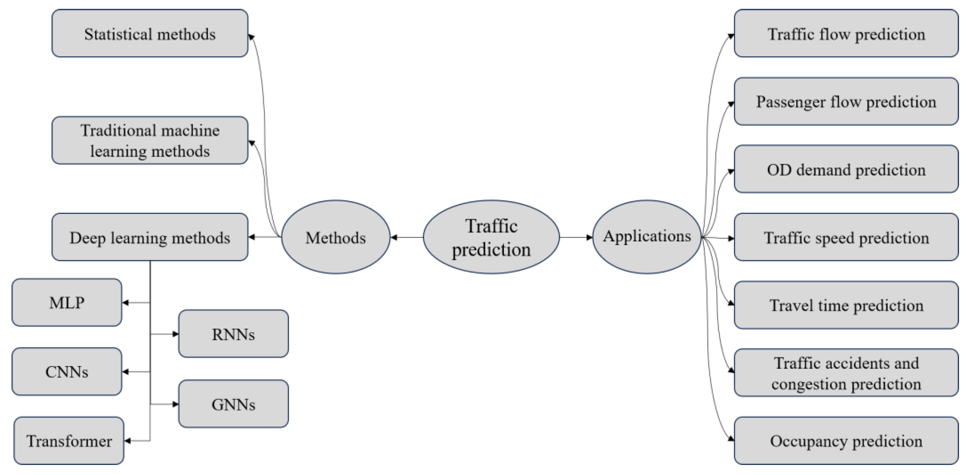
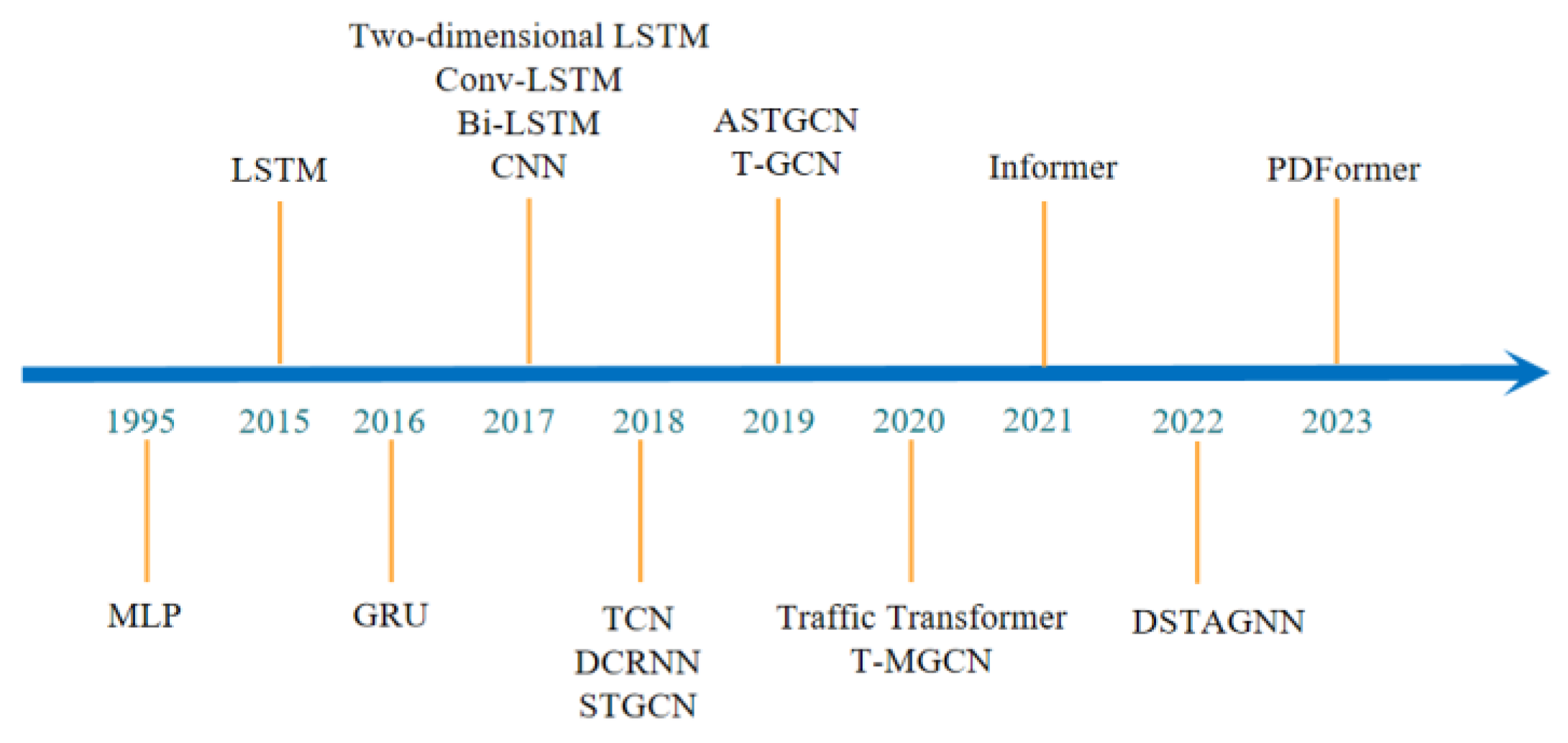
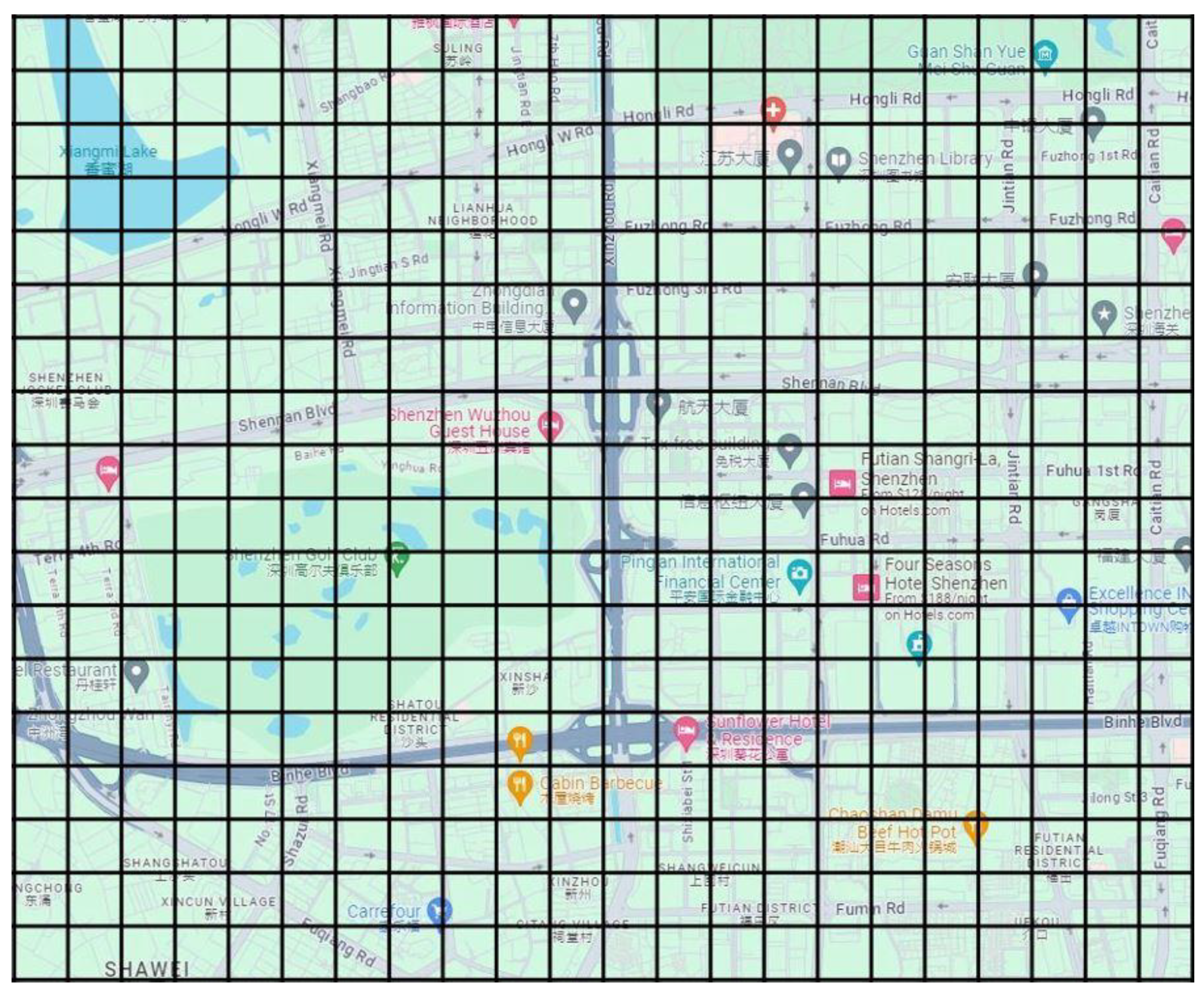
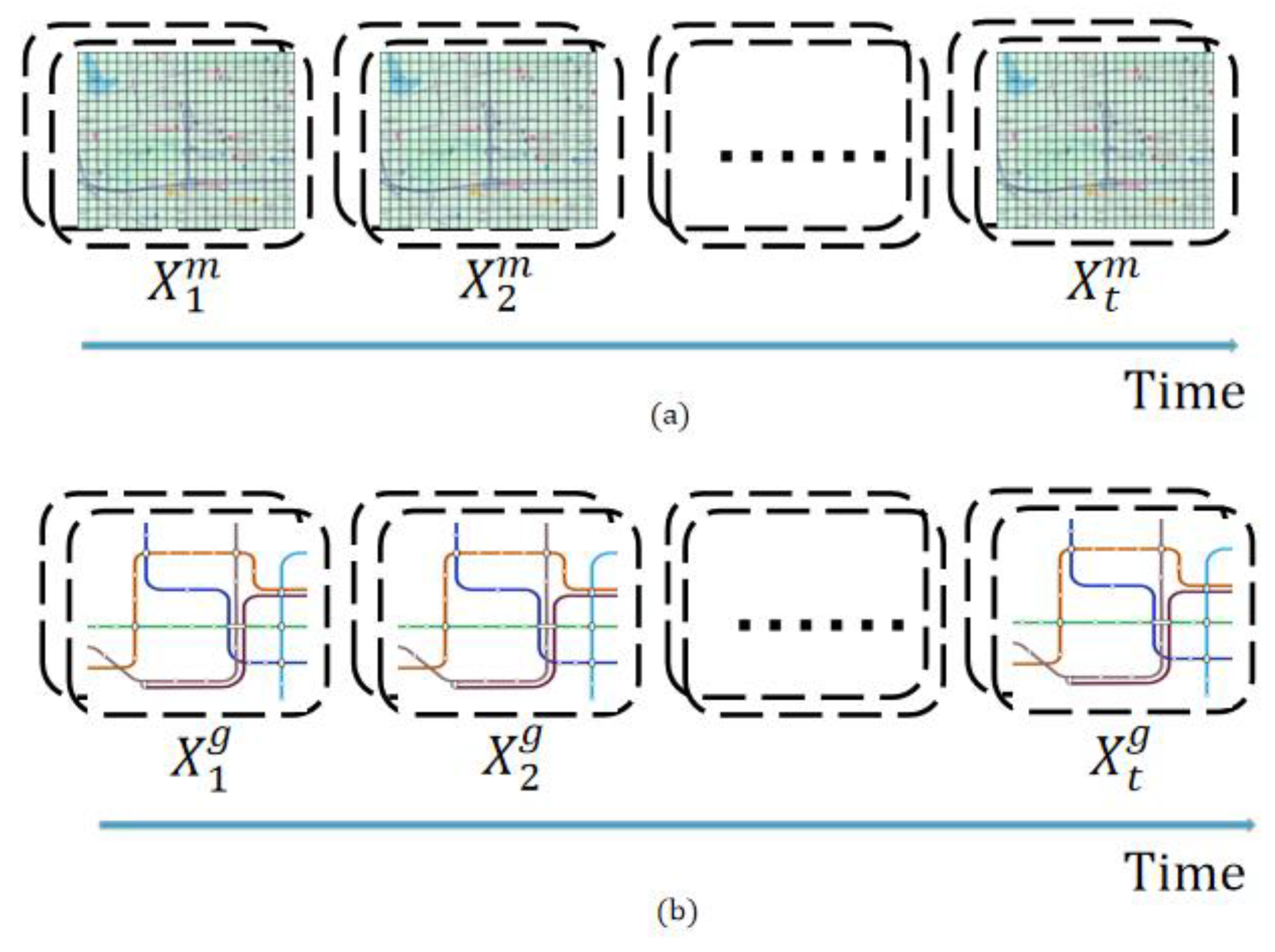

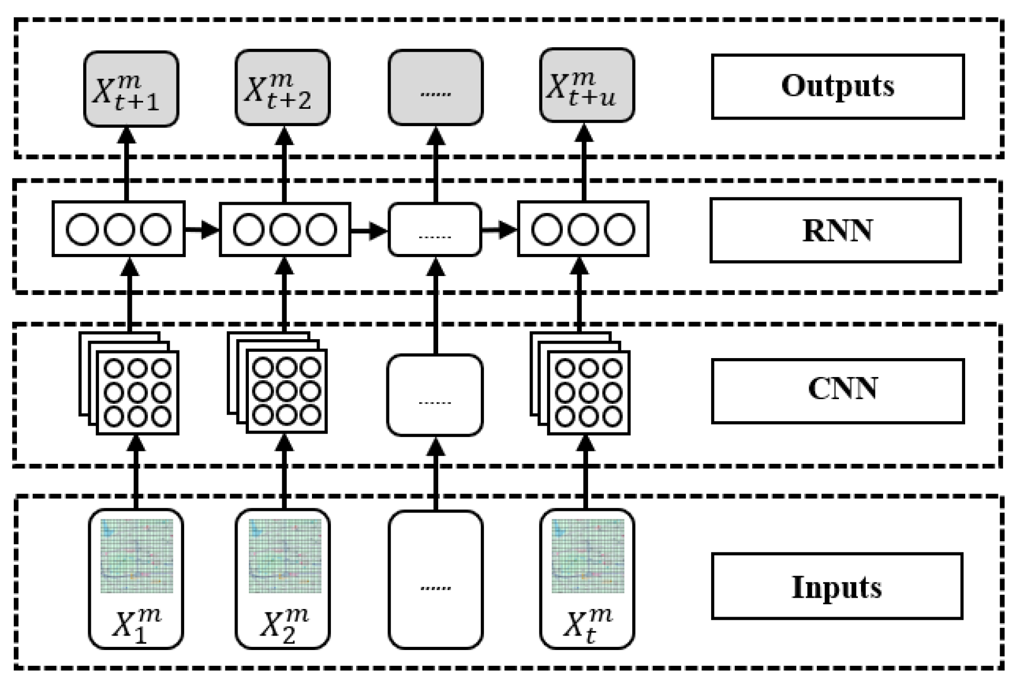
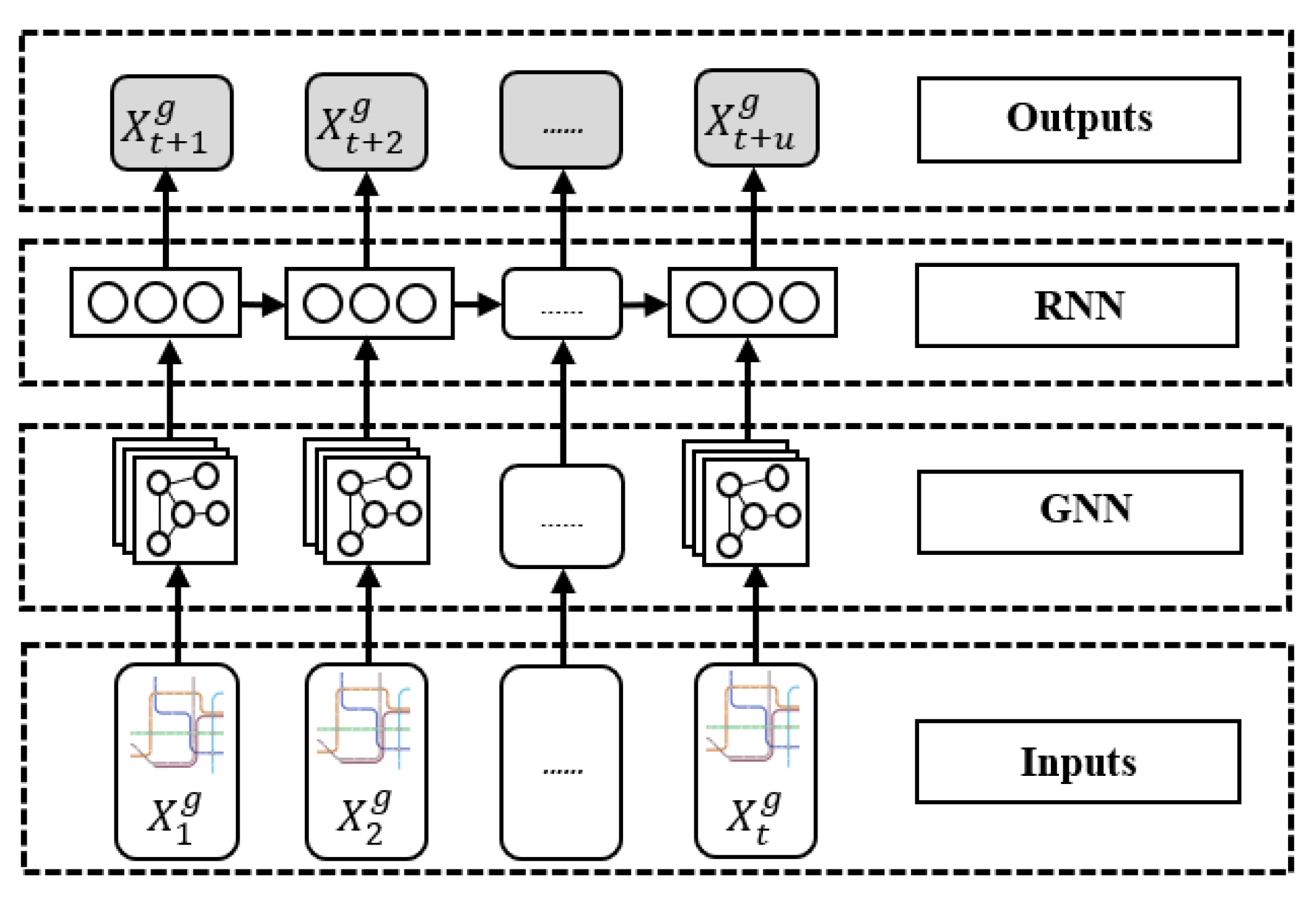
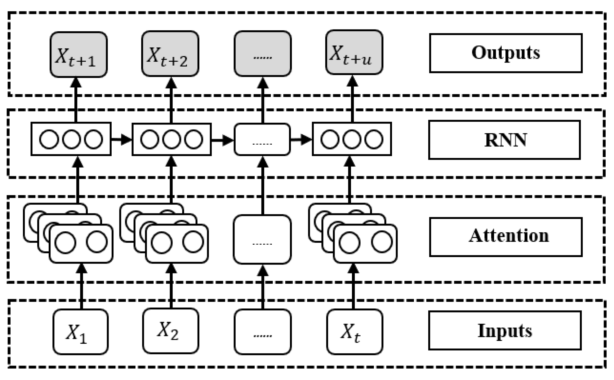
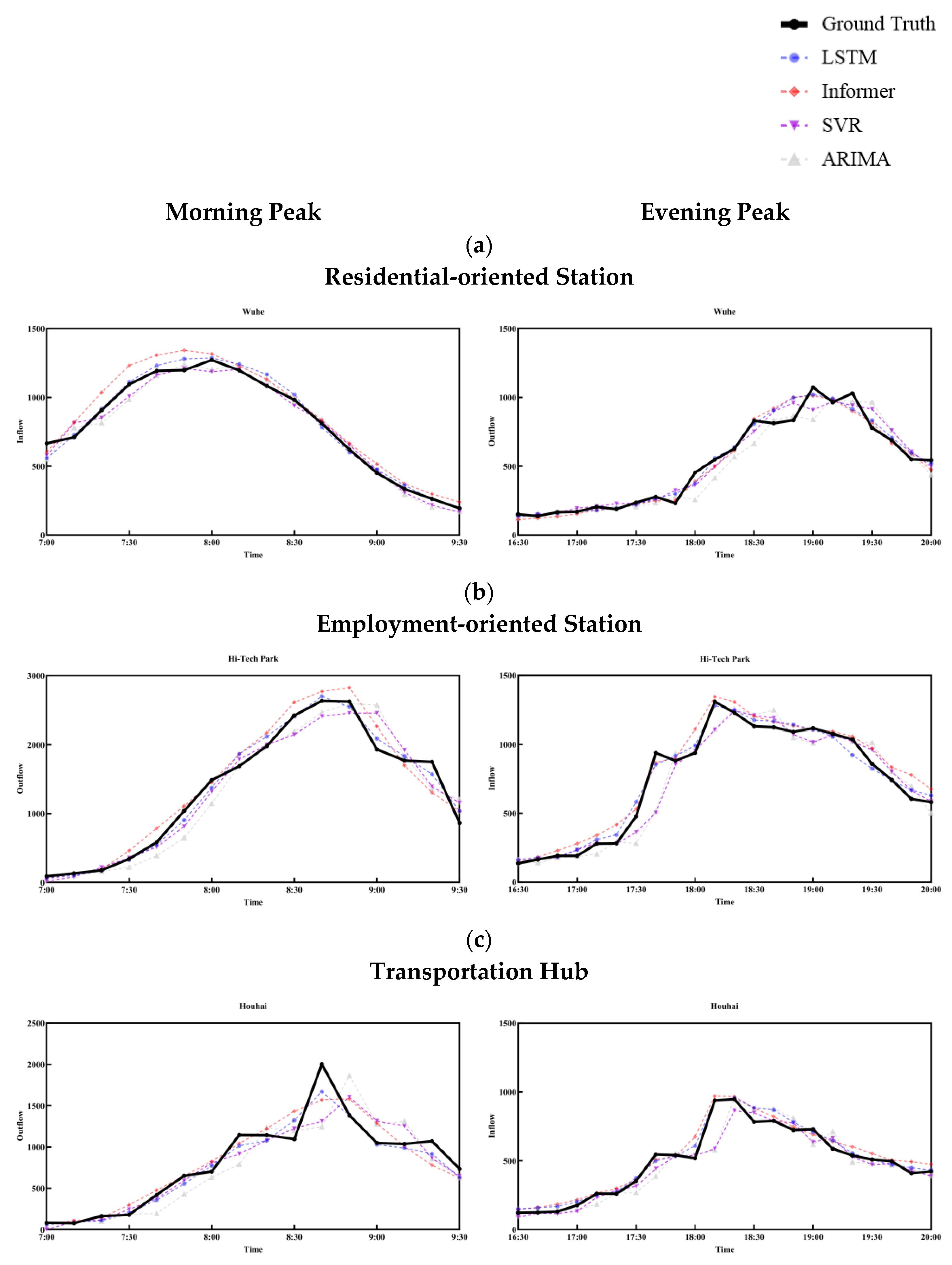
Disclaimer/Publisher’s Note: The statements, opinions and data contained in all publications are solely those of the individual author(s) and contributor(s) and not of MDPI and/or the editor(s). MDPI and/or the editor(s) disclaim responsibility for any injury to people or property resulting from any ideas, methods, instructions or products referred to in the content. |
© 2024 by the authors. Licensee MDPI, Basel, Switzerland. This article is an open access article distributed under the terms and conditions of the Creative Commons Attribution (CC BY) license (https://creativecommons.org/licenses/by/4.0/).