Abstract
Together with the growing interest towards renewable energy sources within the framework of different strategies of various countries, the number of solar power plants keeps growing. However, managing optimal power generation for solar power plants has its own challenges. First comes the problem of work interruption and reduction in power generation. As the system must be tolerant to the faults, the relevance and significance of short-term forecasting of solar power generation becomes crucial. Within the framework of this research, the applicability of different forecasting methods for short-time forecasting is explained. The main goal of the research is to show an approach regarding how to make the forecast more accurate and overcome the above-mentioned challenges using opensource data as features. The data clustering algorithm based on KMeans is proposed to train unique models for specific groups of data samples to improve the generation forecast accuracy. Based on practical calculations, machine learning models based on Random Forest algorithm are selected which have been proven to have higher efficiency in predicting the generation of solar power plants. The proposed algorithm was successfully tested in practice, with an achieved accuracy near to 90%.
1. Introduction
Power generation based on the use of renewable energy sources (RESs) has been developing at a different pace since its first appearance. Before the XX century, it did receive have much attention, and the active development of RES-based generation started with the problem of huge carbon emissions, including greenhouse gasses in the atmosphere [1]. At the beginning of the XXI century, research concluded that a 100% RES electricity supply is feasible worldwide at a low cost [2]. Great attention has also been paid to the fact that all devices used to balance the power supply should use only RES-based power supplies [3].
Currently, Environmental, Social and Governance (ESG) strategies are gaining more importance for the enterprises [4] to controlling carbon emissions, use of energy and preserving the natural resources [5,6].
The current transition of the power industry is defined by the major implementation of RES-based generation and the use of artificial intelligence (AI) technologies to control and operate it. World-leading countries set their goals for achieving 100% carbon-free power systems. One of the first countries in this field was Germany [7], and now at least 48 countries have their own goals according to the COP 22 forum [8,9]. Intergovernmental support of research in this field [10] and the presented results of the International Renewable Energy Agency (IRENA) and the International Energy Agency (IEA) [11,12,13,14,15] makes the concept of a 100% RES-based power industry more feasible. Not only are governmental initiatives [16] accelerating the transition process, but even significant fossil fuel companies, such as British Petroleum, are making steps to reduce their carbon footprint using RES-based power generation [17].
Over the last 10 years, the share of renewable electricity has significantly grown. Today, the highest rates are seen in the capacities of solar and wind power [18,19]. According to statistics from 2022, photovoltaics accounted for 50% of the new installed capacities [20].
However, this technology has its own drawbacks. Along with the growing amount of power plants, interruption of work and reduction in power generation create certain disadvantages for power systems. Grid failures may rise due to the impact of power surpluses or shortages, so it is necessary to build a renewable energy system that is tolerant to these faults. One of the ways to overcome these challenges is to ensure an efficient use of solar power. The possible tool for that is the prediction of PV power generation.
To date, there are two main approaches—the physical one and the statistical one. When developing a physical model, several characteristics are taken into consideration. Those include the influence of solar radiation, the power plant itself, the PV conversion model, the circuit model and the inverter model.
For example, work [21] suggests the prediction method to calculate the parameters and paper [22] proposes the linear system of five equations to assess the above-mentioned parameters. However, due to the changing parameters of the performance of PV models and other challenges, such as changing weather conditions, it becomes difficult to build a physical prediction method.
In comparison to physical models, it is much easier to use a statistical approach, as it is better in catching the probable uncertainties. This method, in turn, can be split into system identification methods and artificial intelligence (AI) approaches, including support vector machines, artificial neural networks and genetic algorithms [23].
Statistical models are based on the analysis of retrospective data to predict changes in the value under consideration [24,25,26,27,28,29]. Statistical models use methods of mathematical statistics, probability distributions, time series, autoregressive models, etc. Models based on artificial intelligence are built on the use of mathematical algorithms to analyze large volumes of data, identify the influence of these data on the predicted value, highlight the most significant ones and use them to calculate the forecast [30,31,32]. Hybrid models, in turn, combine the mechanisms of statistical models, physical approaches to forecasting and artificial intelligence methods. A new area of machine learning research for RES forecasting is the development of explainable AI models [33].
The choice of a forecast model is based on the changing nature of the predicted variable and the available data that can be used to make the forecast. One of the obvious parameters influencing the quality of the forecast and the choice of the forecast model is the forecast horizon [34,35,36]. The forecast horizon determines the future time interval for which the forecast is calculated.
There is no generally accepted classification of forecast horizons. In most cases, three categories are distinguished: short-term, medium-term and long-term forecasts [37,38]. Sometimes a fourth category is introduced—ultra-short-term forecasts [39].
The choice of planning horizon influences the choice of an appropriate model and its accuracy. For long-term forecasting, and in cases where narrow localization of the forecast is not required, it is appropriate to use numerical weather prediction models (if the necessary computing power is available). For short-term forecasts, statistical models, artificial intelligence-based models, and combination models are more suitable [40,41].
PV generation is unstable and sensitive to the weather changes. However, the forecast of the PV generation is crucial for the power system operation and control tasks, and its results should be accurate regardless of weather conditions. Thus, improvements could be provided to this area. This is why the hybrid model, based on clustering of the data using weather features to separate unique weather conditions, can improve the forecasting accuracy. One model (without clustering) has higher chances of overfitting the data because of model complexity. The clustering stage helps to make individual models less complex but more accurately fitted to the data.
In this work, clustering was chosen as the most suitable method to test the hypothesis on the improvement of PV power plant forecasting accuracy. As clustering is one of the forms of data abstraction, we needed to select certain parameters that characterize our objects and then normalize the highlighted characteristics.
Although improvement of forecasting accuracy through the clustering of weather conditions has been studied by many authors, for example [42,43,44,45], there is still a place for improvement in regard to the clustering application for this task. In [42], weather data spread in four groups defined only using meteorological provider labels such as snowy, foggy, sunny and rainy. The authors of [43] applied the DBSCAN method to differentiate clusters in data but divided them by the average value first. In [44], a clustering algorithm was based on only two features (irradiance and temperature). The above-mentioned research barely used any of clustering metrics to evaluate and describe the obtained results, but some authors [45,46] used a silhouette coefficient for evaluation.
The main contributions of this research to the field of PV generation forecasting and weather clustering are as follows:
- Relevant weather features which determine the working state of PV modules were used as initial data for the clustering algorithm;
- Three metrics (silhouette, WSS, and BSS) for data spreading in clusters were used;
- The clustering model was applied to hourly observations to define similar groups of data in terms of the working state of PV modules instead of labeling whole days as rainy or sunny;
This paper’s content is structured as follows. Section 2 presents the applied data preprocessing actions, clustering methods, forecasting models and evaluation metric descriptions. Section 3 shows the obtained results of the research and the comparison of two considered approaches using the described evaluation metrics, providing a discussion. Section 4 provides a discussion on the obtained results and the directions of future work.
2. Materials and Methods
The proposed algorithm includes 11 stages and can be presented as the flow chart in Figure 1.
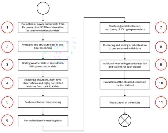
Figure 1.
Flow chart of the proposed algorithm.
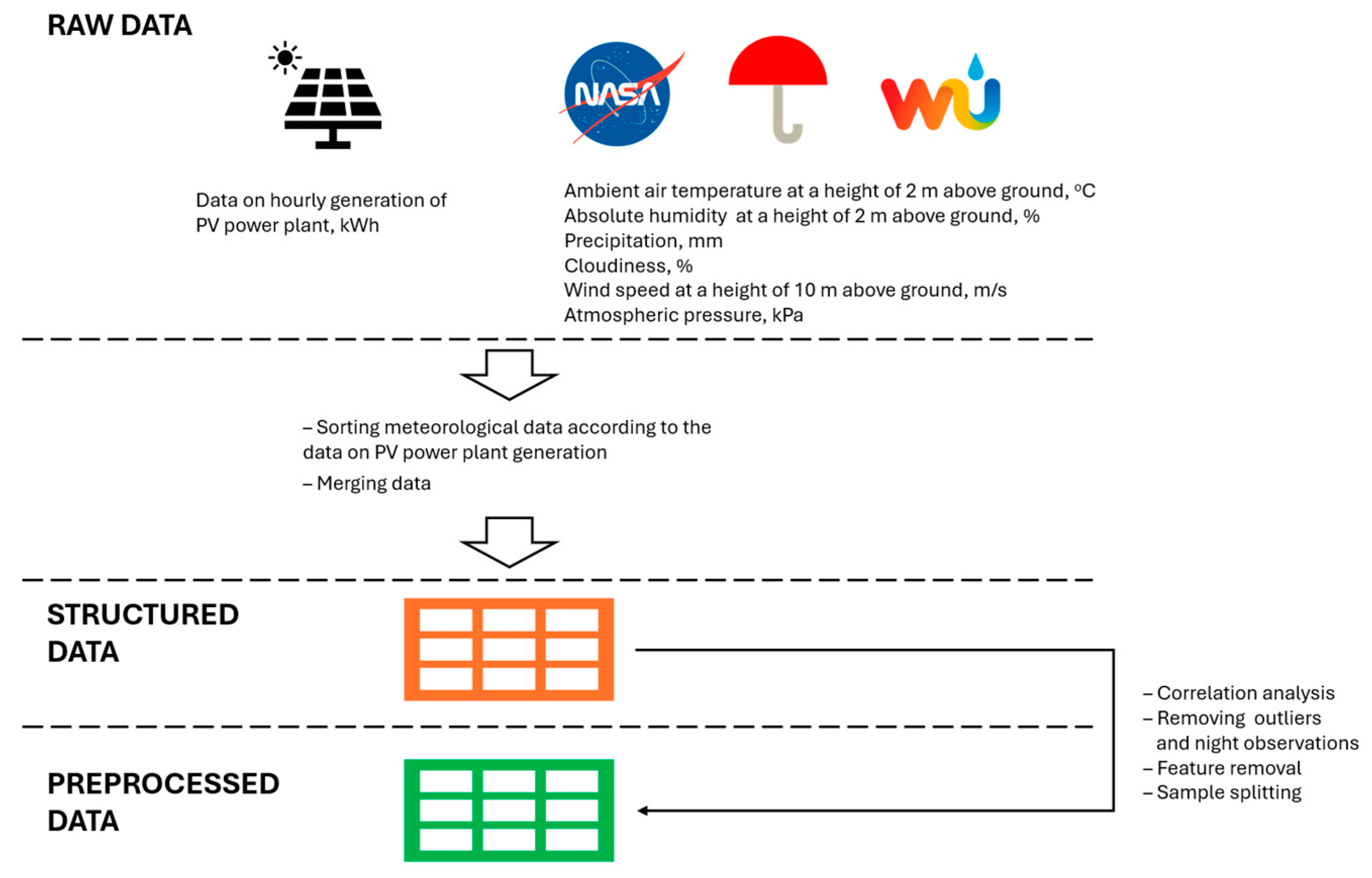
The data preparation stages (Figure 2) were conducted according to the list below:
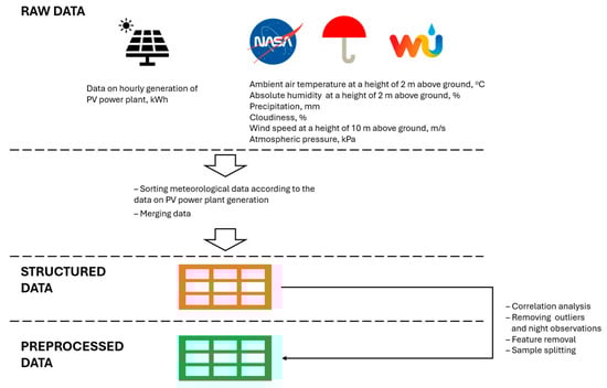
Figure 2.
Data preprocessing stages.
- Data collection from different sources;
- Sorting and merging collected data;
- Removing night observations, outliers, and highly correlated features.
To perform the clustering, four algorithms were tested (KMeans, Agglomerative clustering, Spectral clustering and GaussianMixture) [47]. The distance between data points was calculated using the Euclidean metric:
To compare the clustering results of different models, the following metrics were used:
- Silhouette coefficient (silhouette);
- Between-cluster sum of squares (BSS);
- Within-cluster sum of squares (WSS).
The motive of using all three metrics to evaluate the clustering performance is that, when we use only one of the metrics, we could obtain good numerical values from that metric which correspond to the non-satisfactory results. For example, if we use only the silhouette coefficient, it could be maximized numerically (reaching a value of 1.0), but, at the same time, our cluster borders may become extra complex (may have a weird shape). On the other hand, if we use either the WSS or BSS metric, it could result in a great amount of very small-sized clusters in one case or 1–2 large-sized clusters in another case.
The above metrics were calculated using the following formulas [48]:
where a is the average distance between objects within one cluster; b is the minimum average distance between an object in one cluster and other clusters; ck, cl are the clusters; xi, xj are objects inside the clusters.
The separability of clusters is characterized by the parameter BSS [49] or intercluster distance and is calculated for one cluster as follows:
where M is the number of clusters; ck is the cluster; and xk, xj are the objects inside clusters.
Compactness is characterized by the WSS parameter [49] or intra-cluster distance and is calculated for one cluster as follows:
where ck is the cluster and xi, xj are the objects inside clusters.
The silhouette coefficient ranges from −1 to +1, and the closer it is to +1, the more correct the data separation is considered. The BSS and WSS metrics ranges are not limited and depend on the considered task and data structure.
To build and train a model for predicting the generation and operating modes of a photovoltaic plant, a dataset was collected. It consists of meteorological and geometric parameters of the movement of the Sun, necessary for the physical explanation of the process of propagation of solar radiation. Also, the actual data on the generation of the solar power plant located at the 46th latitude in the Caspian region were used.
Several weather providers were used as sources for obtaining retrospective meteorological data:
- Yandex (Russia) [50];
- WeatherUnderground (United States) [51];
- NasaPower (United States) [52].
It is important to use several weather data sources to minimize errors related to biased data, which may occur if the weather stations are located far away from the considered location. The use of several data sources also helps to diversify the weather data, combining satellite and weather station data. From these sources, data on hourly values of temperature, relative humidity, cloudiness and wind speed were obtained. Retrospective data on hourly solar radiation energy flux densities were obtained from measurements from a local weather station. The solar declination angle was calculated based on the mathematical calculation described below [53].
where is the number of the day in the year.
As a result, a dataset was created containing 9 features and one target variable—generation. The list of parameters included in the source data are presented in Table 1.

Table 1.
A list of parameters included in the source data.
Meteorological data from three sources were averaged and reduced to a one-hour resolution to obtain the most stable and reliable parameters. Meteorological data were collected for a period of one year according to the power generation data time period. In addition, the original dataset was cleared of outliers and omissions in the data. There are descriptions of several functions used in the pseudo code listed below (Algorithm 1):
- drop_empty_strings ()—deletes data samples if there is one or more empty or non-numerical values;
- delete_outliers ()—deletes data samples if outliers are detected using boxplot and quartile distribution in any of the data features;
- min_max_norm ()—rescales feature values to the range between 0 and 1;
- regr_data.P, W1.parameters, etc.—selects particular features (column in the database) to store on received values.
| Algorithm 1. Pseudo Code for Data Preprocessing | |
| Input: P, W1, W2, W3 Output: regr_data, cluster_data Auxiliary variables: counter, sum, Initialization: counter = 0, sum = 0 Begin Data Preprocessing Algorithm | |
| 1 2 3 4 5 6 7 8 9 10 11 12 13 14 15 16 17 18 19 20 21 22 23 24 25 26 27 28 29 30 31 32 33 34 35 | for (p = 1,…, n) do sum = sum + P[p] count = count + 1 if count == 2 do regr_data.P = sum/count count, sum = 0 end if end for for data in regr_data, W1, W2, W3 do data = drop_empty_strings(data) data = delete_outliers(data) end for for h in regr_data.hour do if h in W1.hour do x1 = W1.parameters else x1 = 0 end if if h in W2.hour do x2 = W2.parameters else x2 = 0 end if if h in W3.hour do x3 = W3.parameters else x3 = 0 end if regr_data.parameters = (x1 + x2 + x3)/3 end for cluster_data = [regr_data.Temperature, regr_data.Humidity, regr_data.Wind_speed] for x in cluster_data.parameters do x = x.min_max_norm(x) end for return regr_data, cluster_data |
| End Data Preprocessing Algorithm | |
As a result of the data preprocessing described above, the dimension of the dataset decreased from 11,928 rows to 11,245 rows (6% of the original data volume).
If the initial data are presented in a one-hour resolution and the forecasting horizon is short-term, then the mathematical equation for the abstract forecasting model can be written as follows:
where is the PV generation output for the considered hour; is the particular forecasting model; is the array of meteorological features values for the previous hour.
To train individual models for the selected data clusters, a comparison of the considered types of regression models was made (Linear Regression, Decision Tree Regression, Random Forest Regression).
These models were used to predict solar power plant (SPP) generation and the prediction results were compared as follows:
- The general model was trained on data from all the three clusters;
- Three models for different clusters were trained on the data of these clusters, respectively;
- The forecasting results of the general model were compared to the forecasting results of the composite model (obtained using three models trained on the data of the selected cluster).
To visualize data points in a 2D-space, a principal component analysis (PCA) [54] was used. The PCA method helps to transfer data from higher dimensional space to lower dimensional space and is commonly used for visualization purposes. The main idea of the PCA is to use a linear combination of the original features of the dataset in order of decreasing importance. The PCA process can be described using following steps.
Data standardization:
where is the mean of independent features; is the standard deviation of independent features.
Computation of covariance matrix:
where are the values of two independent features.
Eigenvalues and eigenvectors computation:
where is the eigenvalue.
Data projection to the lower feature space:
where is the vector consisting of the eigenvalues placed in order of decreasing importance.
3. Results and Discussion
A fragment of the generated database for forecasting the generation of solar power plants, obtained as a result of collecting and processing data from weather providers and data on the generation of SPPs, is presented in Table 2. The dimension of the data after removing outliers and clearing the data from non-numeric values and omissions amounted to 5686 rows and 10 columns.
Table 2.
Fragment of the database used to predict the generation of solar power plants.
To divide the source data into clusters in order to increase the accuracy of predicting SPP generation, a set of features was generated. This set consists of the following features from the initial database (Table 2) characterizing meteorological conditions:
- Temperature, actual, °C;
- Humidity, actual, %;
- Wind speed, actual, m/s.
The choice of features is determined not only by their explicit connection to the meteorological conditions but also by the optimal identification of clusters in the data. Thus, the data dimension for creating a clustering model was 5686 rows and three columns. A fragment of the data used for data clustering is presented in Table 3. To select the final clustering model and the optimal number of clusters, four models were compared, namely KMeansClustering, AgglomerativeClustering, SpectralClustering, and GaussianMixture, and various options for the number of allocated clusters were also considered.
Table 3.
Fragment of data used for data clustering.
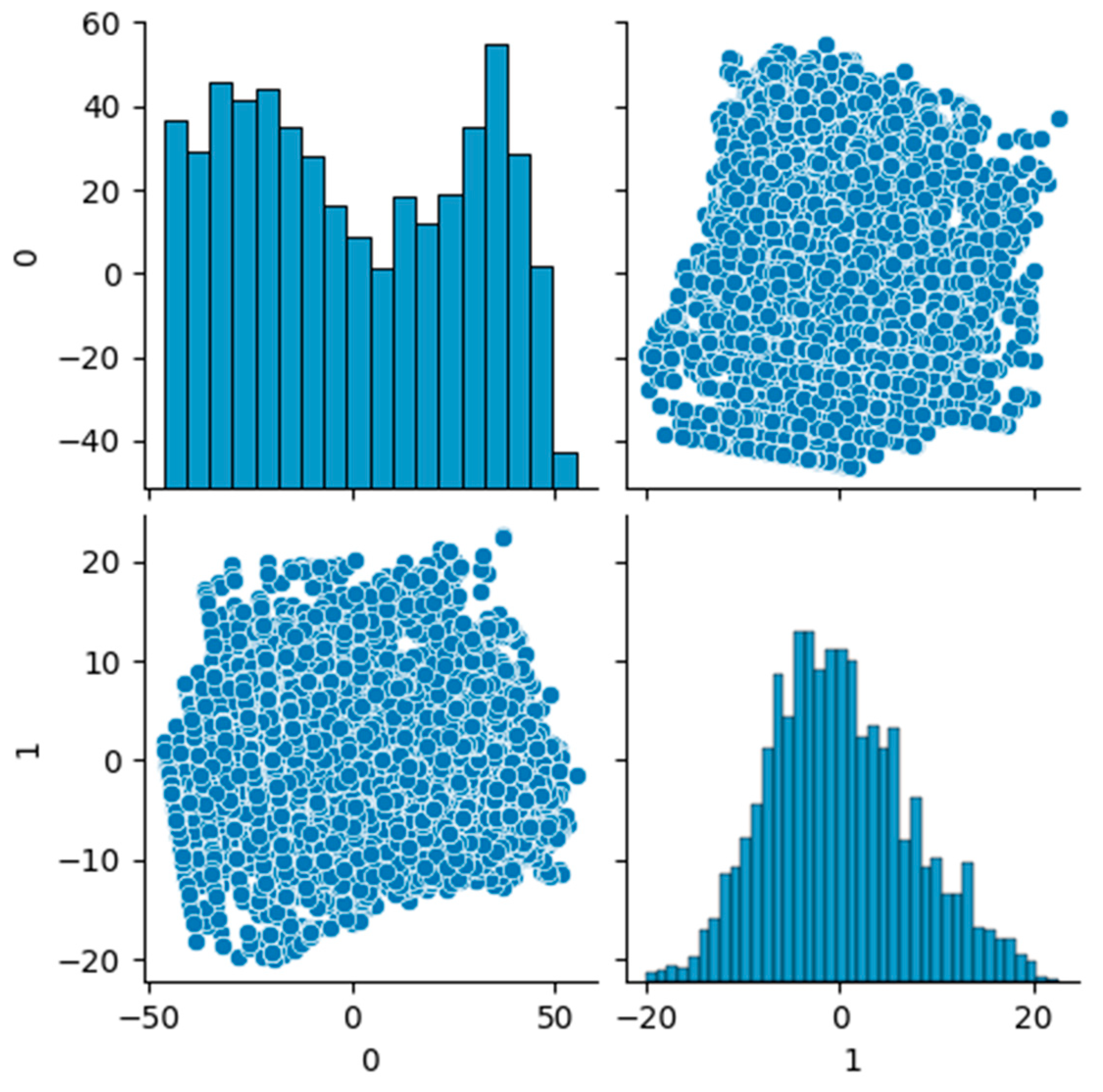
For convenient visualization, the PCA transformation was applied to the data. For the data from Table 2, two principal components were allocated to project the data onto a two-dimensional plane.
As a result of transforming the data into two-dimensional space, their representation was obtained, as shown in Figure 3.
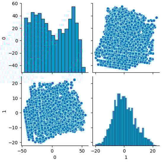
Figure 3.
Data for clustering after transformation into two-dimensional space using the PCA.
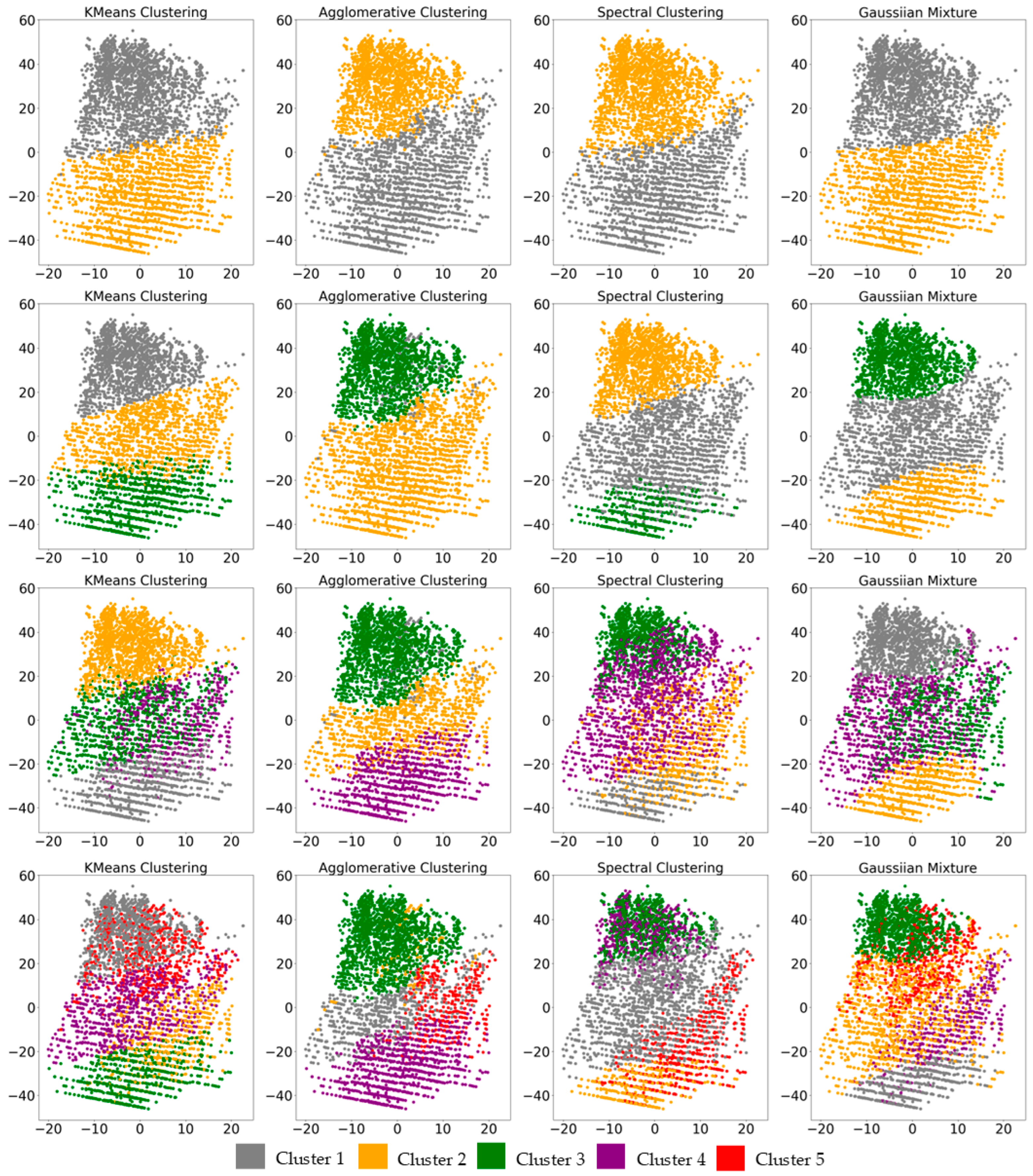
Before applying the selected models for clustering, the data from Table 2 were normalized using a minimax transformation (the data in each column was linearly transformed to range from 0 to 1). Visualization of the results of identifying different numbers of clusters by the considered models is presented in Figure 4, and the values of metrics for each model that determine the optimality of cluster selection are presented in Table 4.
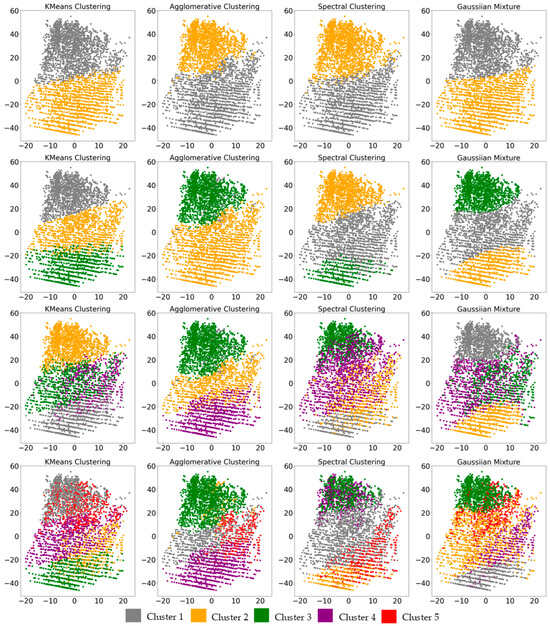
Figure 4.
Clustering results.
Table 4.
Clustering evaluation metrics values.
In accordance with the results of comparing the selection of different numbers of data clusters using the considered models, it was found that the Agglomerative clustering model is not applicable within the framework of the task. The non-applicability of the AG model is expressed visually and numerically. It can be seen in Figure 4 that the AG model provides results featuring one small-sized cluster mixed inside of another bigger cluster in cases where the number of clusters is greater than two. This specific behavior is also expressed in the values of all the metrics used for evaluation in Table 4. The KMeans Clustering, Spectral Clustering and GaussianMixture models showed similar results when identifying different numbers of data clusters (2–5). At the same time, it was determined that the selection of three data clusters in this problem is the optimal solution (the silhouette coefficient is the maximum, and WSS and BSS have the greatest difference).
The averaged separation of KMeans Clustering, SpectralClustering, and GaussianMixture models was adopted as the final model to provide realistic but clearer borders of the identified data clusters.
As a result of clustering, three data clusters of the following dimension were identified:
- First cluster—2120 data lines;
- Second cluster—1977 data lines;
- Third cluster—1588 data lines.
Selected clusters might be considered balanced, since the largest difference between the volumes of the first and third clusters is no more than 25% relative to the cluster with the largest amount of data. In accordance with the identified data clusters, three datasets were generated for training regression models to predict the generation of SPPs. A separate dataset was obtained from the original data by randomly selecting samples. This set was limited in size to accommodate the sample sizes based on the identified clusters. Thus, 1980 data samples were randomly selected from the original data, which corresponds to the volumes of the selected clusters.
Each dataset was divided into training and testing sets in a ratio of 80/20. Information on the sampling structure for each of the three sets is presented in Table 5.
Table 5.
Structure of training and test samples for the four datasets.
Based on the comparison results (Figure 5, Figure 6, Figure 7 and Figure 8 and Table 6, Table 7, Table 8 and Table 9), Random Forest Regression was selected as a predictive model for further tuning. As a result of tuning the models using the Exhaustive search method in order to increase accuracy, four sets of parameters for predictive models were identified:
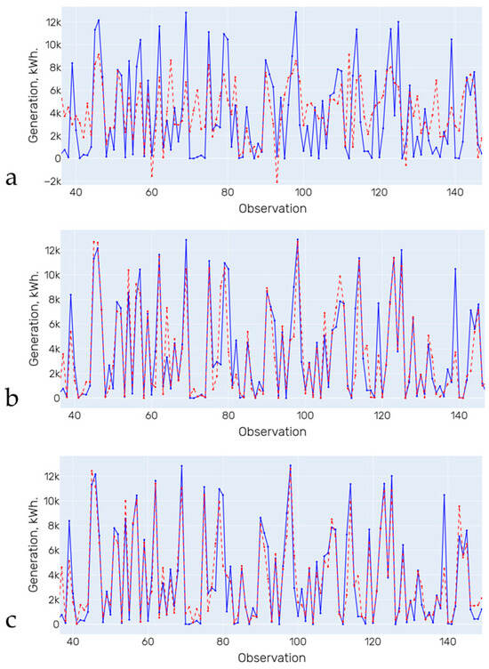
Figure 5.
Forecasting results (training on initial data). (a)—Linear Regression; (b)—Decision Tree; (c)—Random Forest. Blue line is the actual data, red line is the forecasting results.
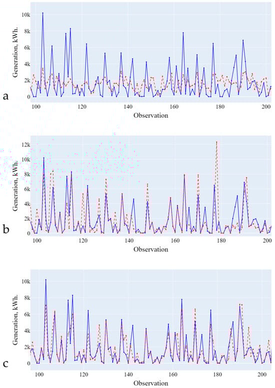
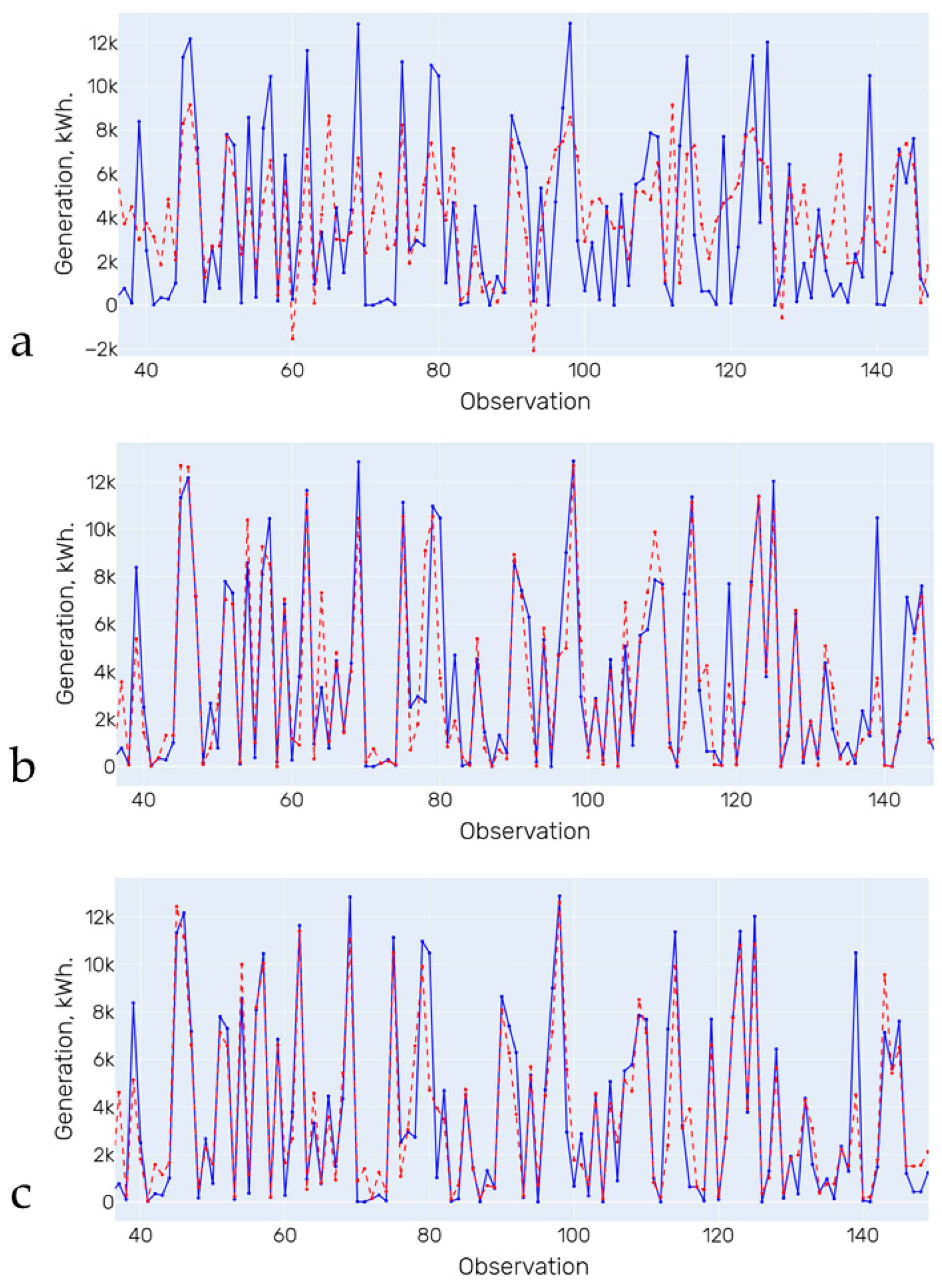
Figure 6.
Forecasting results (training on data from the first cluster). (a)—Linear Regression; (b)—Decision Tree; (c)—Random Forest. Blue line is the actual data, red line is the forecasting results.
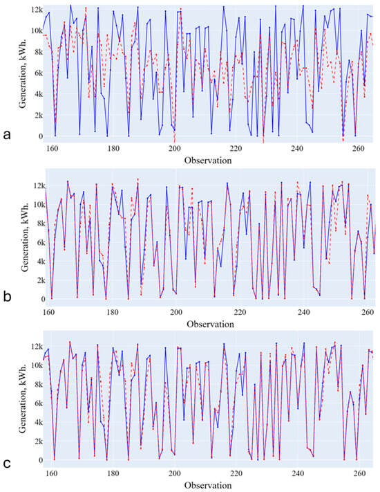
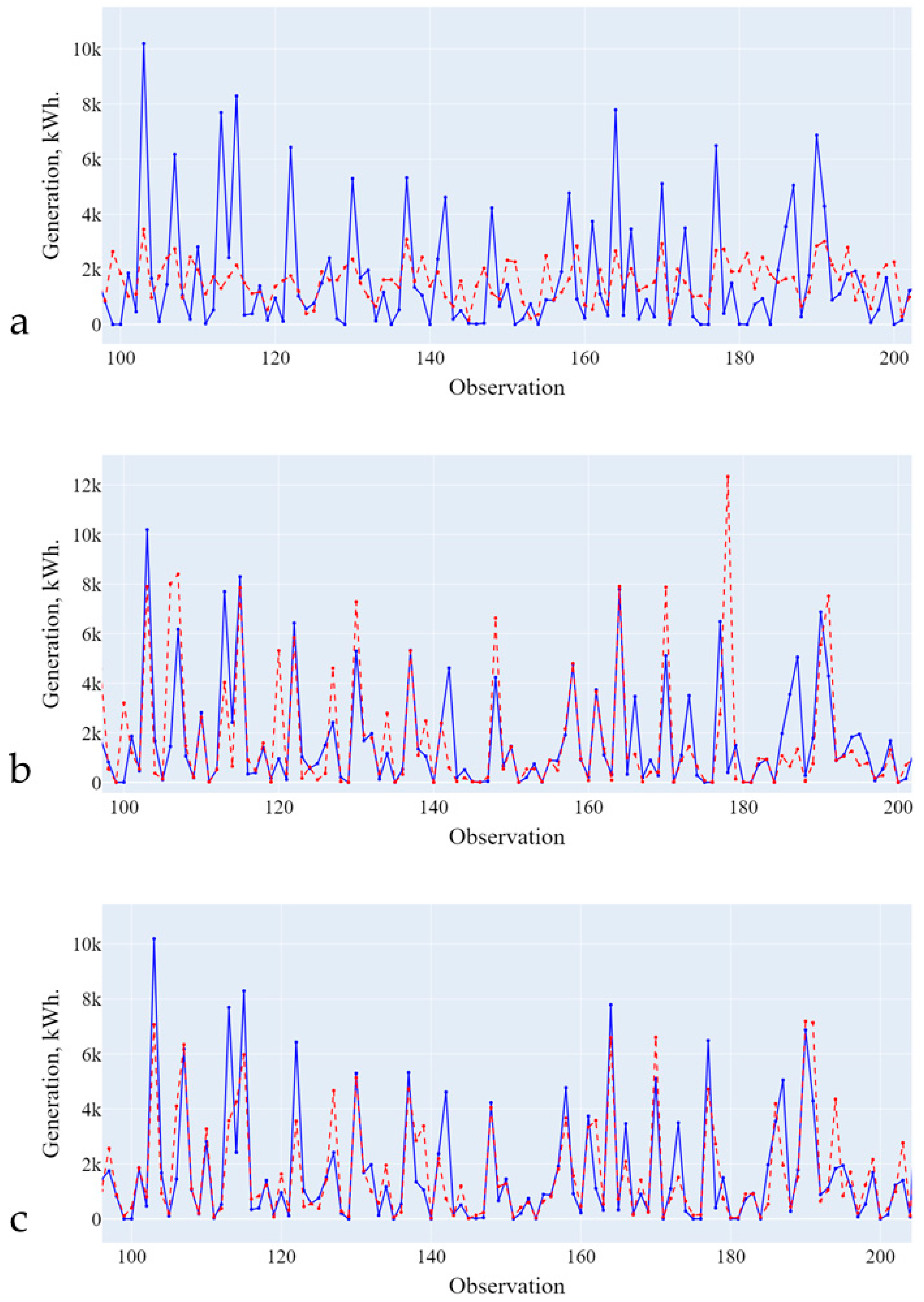
Figure 7.
Forecasting results (training on data from the second cluster). (a)—Linear Regression; (b)—Decision Tree; (c)—Random Forest. Blue line is the actual data, red line is the forecasting results.
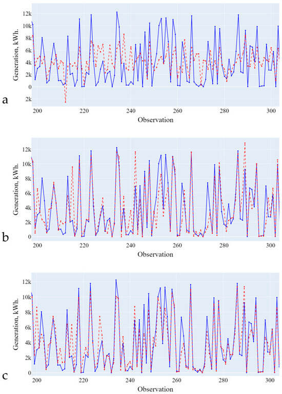
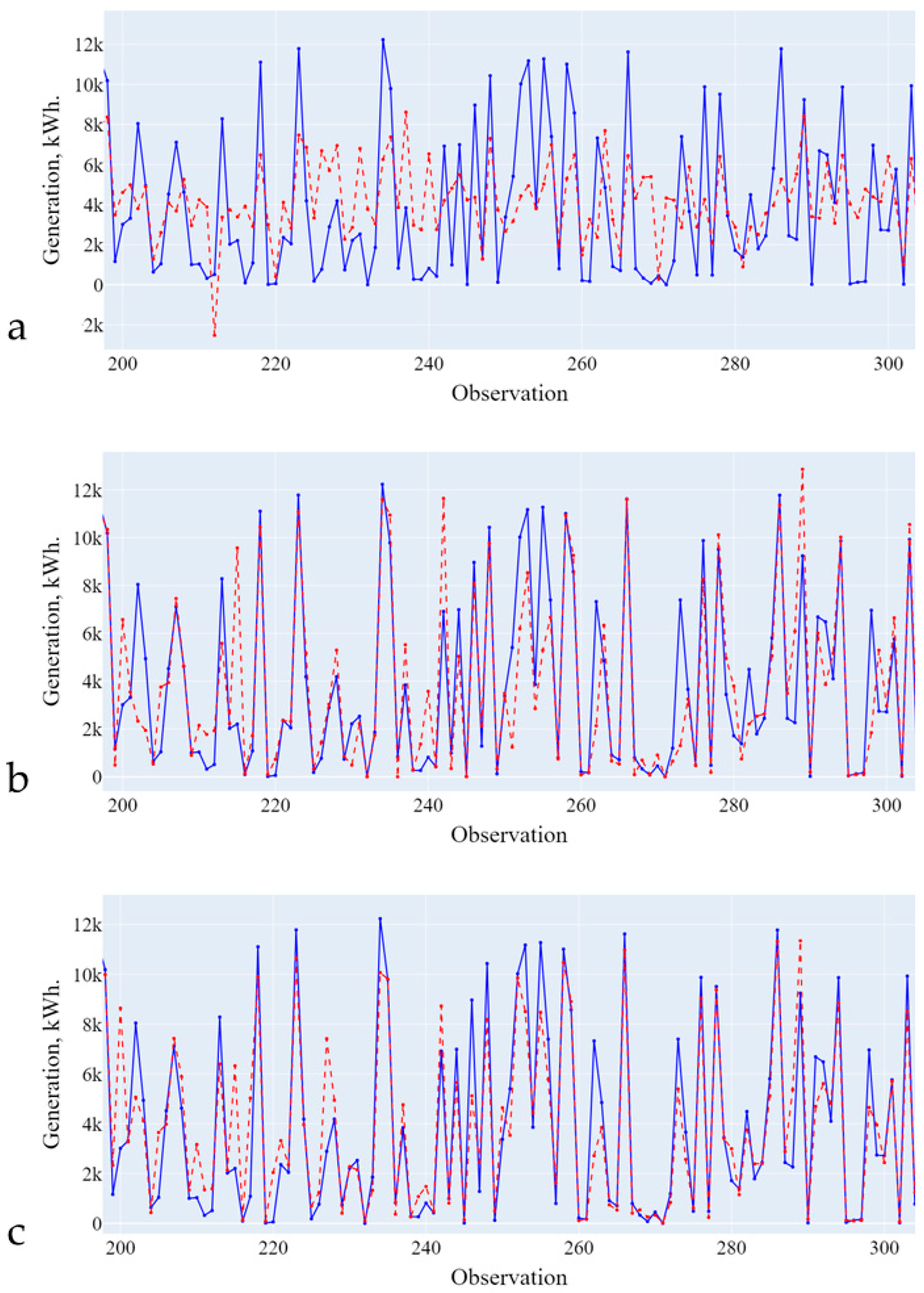
Figure 8.
Forecasting results (training on data from the third cluster). (a)—Linear Regression; (b)—Decision Tree; (c)—Random Forest. Blue line is the actual data, red line is the forecasting results.
Table 6.
Forecasting results (trained on initial data).
Table 7.
Forecasting results (trained on data from the first cluster).
Table 8.
Forecasting results (trained on data from the second cluster).
Table 9.
Forecasting results (trained on data from the third cluster).
- General model: (‘criterion’: ‘poisson’, ‘max_features’: 4, ‘n_estimators’: 115);
- Model for the first cluster: (‘criterion’: ‘poisson’, ‘max_features’: 4, ‘n_estimators’: 87);
- Model for the second cluster: (‘criterion’: ‘poisson’, ‘max_features’: 4, ‘n_estimators’: 73);
- Model for the third cluster: (‘criterion’: ‘poisson’, ‘max_features’: 4, ‘n_estimators’: 132).
Training separate models for each of the selected clusters and using them together instead of one common model trained on all data will lead to increased accuracy in predicting SPP generation. In this case, the accuracy of the final forecast may decrease due to a decrease in the size of the training sample for each model. This negative impact will disappear with a subsequent increase in retrospective data for the forecasting system.
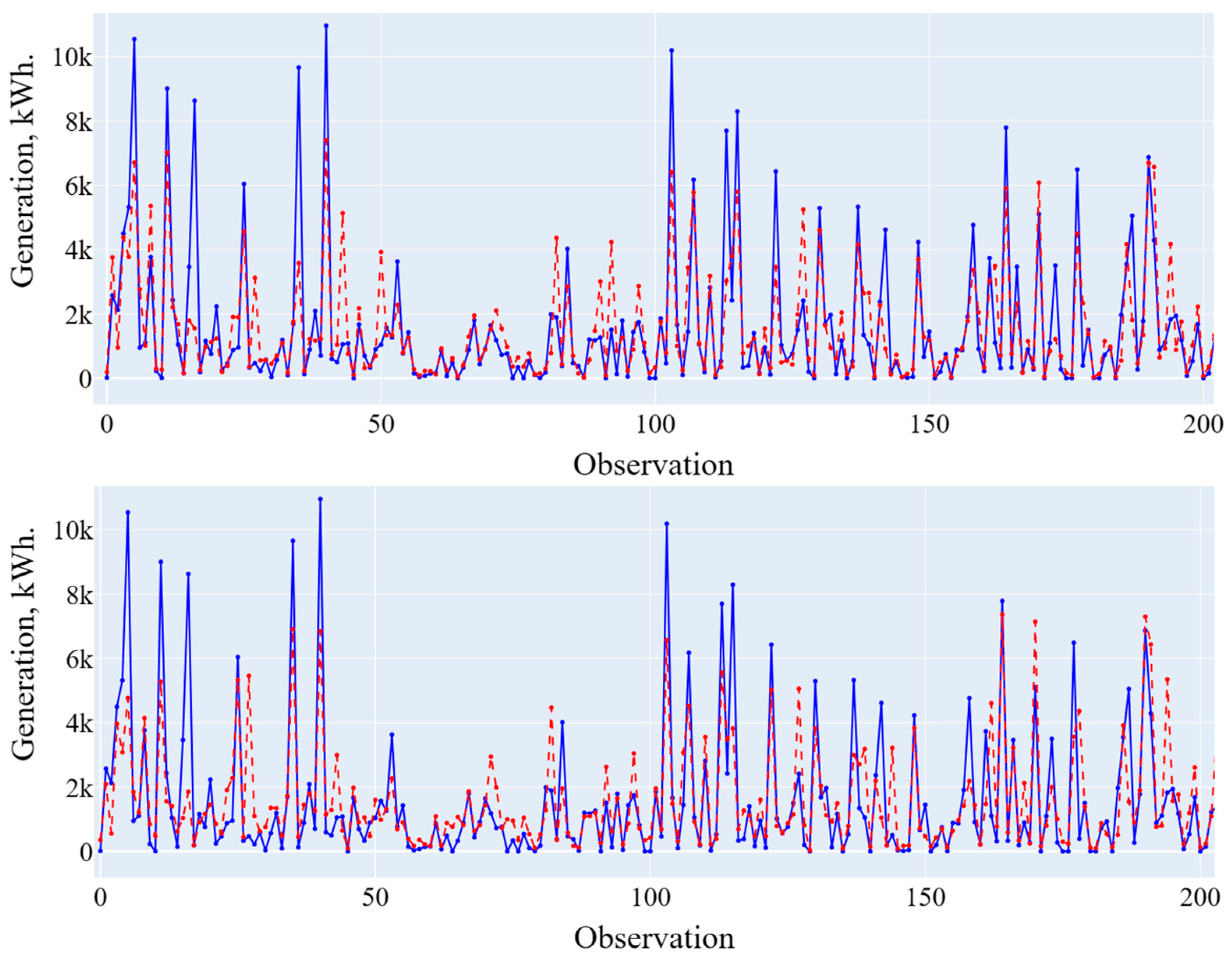
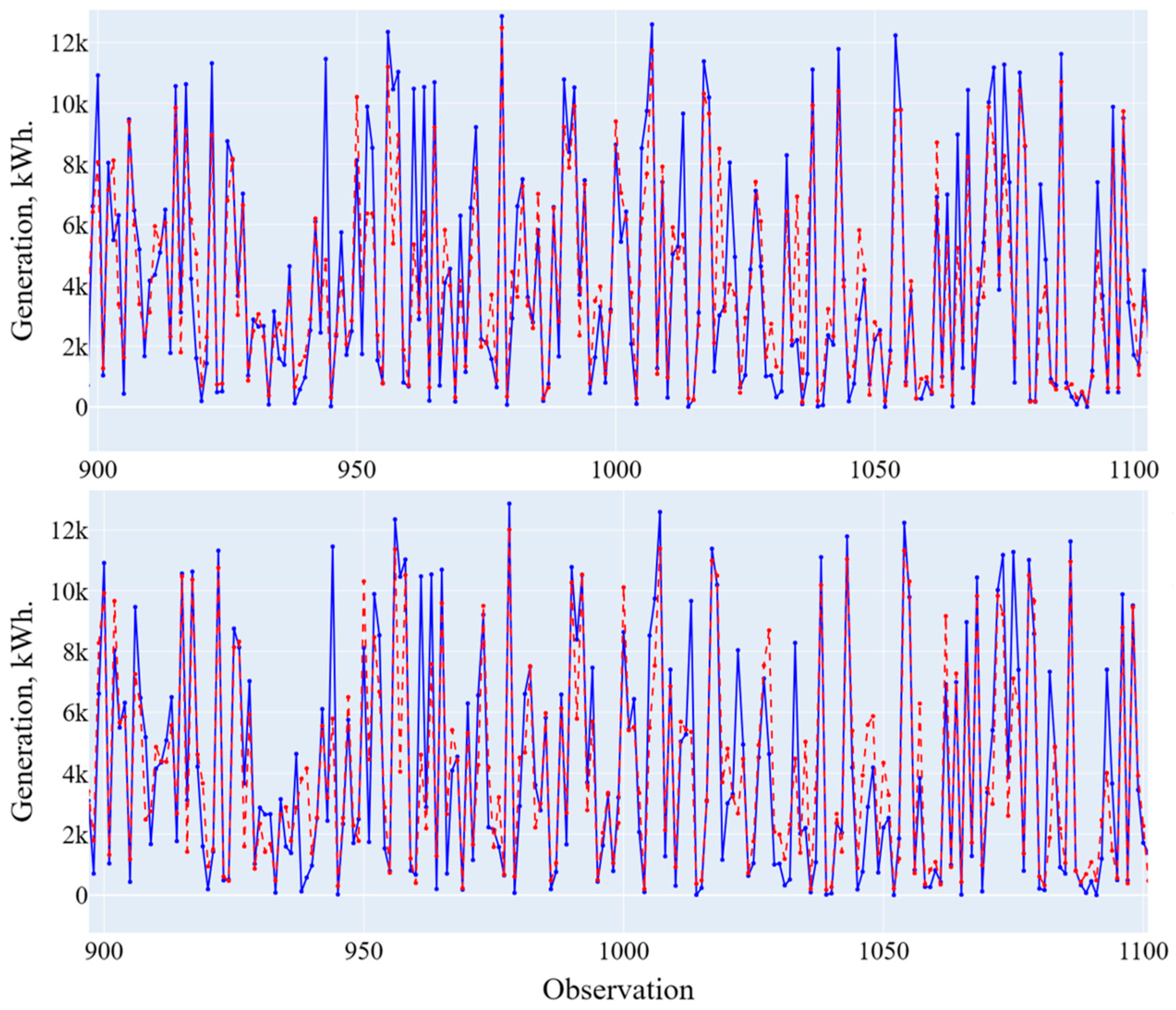
The results of forecasting two models, general and composite (from three models), and their comparison are presented in Figure 9 and Figure 10 and Table 10.
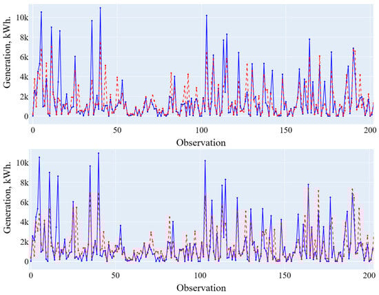
Figure 9.
Forecasting results using a general and composite model (low generation level). Blue line is the actual data, red line is the forecasting results.
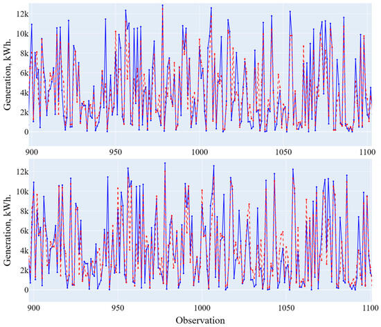
Figure 10.
Forecasting results using a general and composite model (high generation level). Blue line is the actual data, red line is the forecasting results.
Table 10.
Comparison of the forecasting results using a general and composite model.
4. Conclusions
The study found that training separate models for each of the selected data clusters significantly improves the accuracy of forecasting solar power plant (SPP) generation. It is important to note that the model trained on the original data showed even lower accuracy compared to the model for the second cluster. Thus, to achieve higher results in predicting solar power generation, it is necessary to consider the data volumes and their quality when choosing a suitable model. Thus, the approach with the use of separate models for clusters seems more promising.
The obtained results show that the composite model provided a reduction in the nMAE of the forecast that was nearly twice that of the general model and a minor improvement in terms of other considered metrics. These improvements were obtained due to data clustering and tuning the individual models for each cluster. The first cluster contains mostly data observations related to the winter and autumn period with medium level humidity (50–70%). The second cluster data are characterized with lower level humidity (below 50%), and there are no winter data. The third cluster contains data related to high-level humidity (close to 100%) and represents rainy or snowy days mostly. Tuning of the individual models helps to target specific features of each cluster better than through one model exclusively. The individual models are less complex than one general model at the same time. This helps to avoid overfitting and to increase the accuracy.
The general model still provides acceptable results on average and can be used for the territories where the weather is close to stable during the whole year. However, for the territories with changing weather and well-defined climatic seasons, it is recommended to use composite models.
The main contributions of this research in comparison with other studies are using weather features which describe the surrounding effects of the working state of the PV modules; clustering each observation (one hour resolution) instead of clustering days; and evaluation of clustering results with appropriate metrics (silhouette coefficient, BSS and WSS).
Additionally, the use of individual models for each cluster may have some disadvantages, such as the training sample size for each model decreasing with number of the clusters increasing and the underperformance of this approach due to the number of clusters being too high or too low. In further research, the negative effects of the proposed approach may be eliminated with the collection of more retrospective data, control of the adequate number of clusters, and exploring additional features that will affect the clustering process positively.
Author Contributions
Conceptualization, A.M.B. and S.A.E.; methodology, K.I.H., A.M.B. and P.V.M.; software, K.I.H. and A.M.B.; validation, A.M.B. and S.A.E.; formal analysis, P.V.M.; investigation, A.M.B. and S.A.E.; writing—original draft preparation, K.I.H.; writing—review and editing, A.M.B. and P.V.M.; visualization, K.I.H.; supervision, S.A.E. and P.V.M. All authors have read and agreed to the published version of the manuscript.
Funding
The research was carried out within the state assignment with the financial support of the Ministry of Science and Higher Education of the Russian Federation (subject No. FEUZ-2022-0030 Development of an intelligent multi-agent system for modeling deeply integrated technological systems in the power industry).
Data Availability Statement
Dataset available on request from the authors.
Conflicts of Interest
The authors declare no conflicts of interest.
References
- Halicioglu, F.; Ketenci, N. Output, renewable and non-renewable energy production, and international trade: Evidence from EU-15 countries. Energy 2018, 159, 995–1002. [Google Scholar] [CrossRef]
- Breyer, C.; Khalili, S.; Bogdanov, D.; Ram, M.; Oyewo, A.S.; Aghahosseini, A.; Gulagi, A.; Solomon, A.A.; Keiner, D.; Lopez, G.; et al. On the History and Future of 100% Renewable Energy Systems Research. IEEE Access 2022, 10, 78176–78218. [Google Scholar] [CrossRef]
- Irena Coalition for Action. Available online: https://coalition.irena.org/?_gl=1*faxigk*_ga*OTc2OTU0OTMwLjE3MTQ0NjU3ODY.*_ga_7W6ZEF19K4*MTcxNDQ2NTc4Ni4xLjEuMTcxNDQ2NTg5MC40My4wLjA (accessed on 16 August 2024).
- Leong, W.Y.; Leong, Y.Z.; Leong, W.S. Smart Manufacturing Technology for Environmental, Social, and Governance (ESG) Sustainability. In Proceedings of the 5th Eurasia Conference on IOT, Communication and Engineering (ECICE), Yunlin, Taiwan, 27–29 October 2023. [Google Scholar] [CrossRef]
- Biasin, M.; Foglie, A.D.; Giacomini, E. Addressing climate challenges through ESG-real estate investment strategies: An asset allocation perspective. Financ. Res. Lett. 2024, 63, 105381. [Google Scholar] [CrossRef]
- Ayadi, F.; Colak, I.; Garip, I.; Bulbul, H.I. Targets of Countries in Renewable Energy. In Proceedings of the 2020 9th International Conference on Renewable Energy Research and Application (ICRERA), Glasgow, UK, 27–30 September 2020. [Google Scholar] [CrossRef]
- International Energy Agency. Energy Policies of IEA Countries: Denmark 2011 Review. Available online: https://iea.blob.core.windows.net/assets/3df26d26-9271-490b-ae10-1e9a14350412/EnergyPoliciesofIEACountriesDenmark2011.pdf (accessed on 6 August 2024).
- Climate Vulnerable Forum. Geneva, Rotterdam, Accra. Available online: https://thecvf.org/about/ (accessed on 6 August 2024).
- Renewable Energy Policy Network for the 21st Century. Renewables 2020 Global Status Report. Available online: https://build-up.ec.europa.eu/sites/default/files/content/gsr_2020_full_report_en.pdf (accessed on 30 April 2024).
- IPCC. Intergovernmental Panel on Climate Change. Global Warming of 1.5 °C. Available online: https://www.ipcc.ch/site/assets/uploads/sites/2/2019/06/SR15_Full_Report_High_Res.pdf (accessed on 6 August 2024).
- International Renewable Energy Agency. Towards 100% Renewable Energy: Status, Trends and Lessons Learned. Available online: https://coalition.irena.org/-/media/Files/IRENA/Coalition-for-Action/IRENA_Coalition_100percentRE_2019.pdf (accessed on 6 August 2024).
- International Renewable Energy Agency. Towards 100% Renewable Energy: Utilities in Transition. Available online: https://www.irena.org/Publications/2020/Jan/Towards-100-percent-renewable-energy-Utilities-in-transition (accessed on 6 August 2024).
- International Renewable Energy Agency. Antigua & Barbuda Renewable Energy Roadmap. Available online: https://www.irena.org/-/media/Files/IRENA/Agency/Publication/2021/March/IRENA_Antigua_Barbuda_RE_Roadmap_2021.pdf (accessed on 6 August 2024).
- International Energy Agency. Net Zero by 2050: A Roadmap for the Global Energy Sector. Available online: https://www.iea.org/reports/net-zero-by-2050 (accessed on 6 August 2024).
- International Energy Agency. Conditions and Requirements for the Technical Feasibility of a Power System with a High Share of Renewables in France towards 2050. Available online: https://www.iea.org/reports/conditions-and-requirements-for-the-technical-feasibility-of-a-power-system-with-a-high-share-of-renewables-in-france-towards-2050 (accessed on 6 August 2024).
- European Commission. A Clean Planet for All—A European Strategic Long-Term Vision for a Prosperous, Modern, Competitive and Climate Neutral Economy. Available online: https://eur-lex.europa.eu/legal-content/EN/TXT/?uri=CELEX%3A52018DC0773 (accessed on 6 August 2024).
- Energy Outlook, BP PLC. Available online: https://www.bp.com/en/global/corporate/energy-economics/energy-outlook.html (accessed on 6 August 2024).
- International Renewable Energy Agency. Renewable Capacity Statistics. Available online: https://www.irena.org/Publications/2024/Mar/Renewable-capacity-statistics-2024 (accessed on 6 August 2024).
- Haegel, N.M.; Kurtz, S.R. Global progress toward renewable electricity: Tracking the role of solar. IEEE J. Photovolt. 2021, 11, 1335–1342. [Google Scholar] [CrossRef]
- The Energy Institute. Statistical Review of World Energy. Available online: https://www.energyinst.org/statistical-review (accessed on 6 August 2024).
- Chatterjee, A.; Keyhani, A.; Kapoor, D. Identification of photovoltaic source models. IEEE Trans. Energy Convers. 2011, 26, 883–889. [Google Scholar] [CrossRef]
- Celik, A.N.; Acikgoz, N. Modelling and experimental verification of the operating current of mono-crystalline photovoltaic modules using four- and five-parameter models. Appl. Energy 2007, 84, 1–15. [Google Scholar] [CrossRef]
- Li, X.; Wu, R.; Gao, Y.; Zheng, Z.A. Power Prediction System for Photo-Voltaic Power Plants. In Proceedings of the 2nd IEEE Conference on Energy Internet and Energy System Integration (EI2), Beijing, China, 20–22 October 2018; pp. 1–6. [Google Scholar] [CrossRef]
- Prema, V.; Rao, K.U. Development of statistical time series models for solar power prediction. Renew. Energy 2015, 83, 100–109. [Google Scholar] [CrossRef]
- Talari, S.; Shafie-Khah, M.; Osório, G.J.; Aghaei, J.; Catalão, J.P. Stochastic modelling of renewable energy sources from operators’ point of-view: A survey. Renew. Sustain. Energy Rev. 2018, 81, 1953–1965. [Google Scholar] [CrossRef]
- Dai, H.; Zhang, N.; Su, W. A Literature Review of Stochastic Programming and Unit Commitment. J. Power Energy Eng. 2015, 3, 206–214. [Google Scholar] [CrossRef]
- Aien, M.; Rashidinejad, M.; Firuz-Abad, M.F. Probabilistic power flow of correlated hybrid wind-PV power systems. IET Renew. Power Gener. 2014, 8, 649–658. [Google Scholar] [CrossRef]
- Zachary, S.; Dent, C.J. Probability theory of capacity value of additional generation. J. Risk Reliab. 2012, 226, 33–43. [Google Scholar] [CrossRef]
- Ioannou, A.; Angus, A.; Brennan, F. Risk-based methods for sustainable energy system planning: A review. Renew. Sustain. Energy Rev. 2017, 74, 602–615. [Google Scholar] [CrossRef]
- Monteiro, C.; Santos, T.; Fernandez-Jimenez, L.A.; Ramirez-Rosado, I.J.; Terreros-Olarte, M.S. Short-term power forecasting model for photovoltaic plants based on historical similarity. Energies 2013, 6, 2624–2643. [Google Scholar] [CrossRef]
- Zeng, J.; Qiao, W. Short-term solar power prediction using a support vector machine. Renew. Energy 2013, 52, 118–127. [Google Scholar] [CrossRef]
- Persson, C.; Bacher, P.; Shiga, T.; Madsen, H. Multi-site solar power forecasting using gradient boosted regression trees. Sol. Energy 2017, 150, 423–436. [Google Scholar] [CrossRef]
- Matrenin, P.V.; Gamaley, V.V.; Khalyasmaa, A.I.; Stepanova, A.I. Solar Irradiance Forecasting with Natural Language Processing of Cloud Observations and Interpretation of Results with Modified Shapley Additive Explanations. Algorithms 2024, 17, 150. [Google Scholar] [CrossRef]
- Raza, M.Q.; Nadarajah, M.; Ekanayake, C. On recent advances in PV output power forecast. Sol. Energy 2016, 136, 125–144. [Google Scholar] [CrossRef]
- Nespoli, A.; Ogliari, E.; Leva, S.; Pavan, A.M.; Mellit, A.; Lughi, V.; Dolara, A. Day-ahead photovoltaic forecasting: A comparison of the most effective techniques. Energies 2019, 12, 1621. [Google Scholar] [CrossRef]
- Sobri, S.; Koohi-Kamali, S.; Rahim, N.A. Solar photovoltaic generation forecasting methods: A review. Energy Convers. Manag. 2018, 156, 459–497. [Google Scholar] [CrossRef]
- Raza, M.Q.; Khosravi, A. A review on artificial intelligence based load demand forecasting techniques for smart grid and buildings. Renew. Sustain. Energy Rev. 2015, 50, 1352–1372. [Google Scholar] [CrossRef]
- Rodrigo, A.M.; Bello, A.; Reneses, J. Electricity price forecasting in the short term hybridising fundamental and econometric modelling. Electr. Power Syst. Res. 2019, 167, 240–251. [Google Scholar] [CrossRef]
- Ren, Y.; Suganthan, P.N.; Srikanth, N. Ensemble methods for wind and solar power forecasting—A state-of-the-art review. Renew. Sustain. Energy Rev. 2015, 50, 82–91. [Google Scholar] [CrossRef]
- Liu, Y. A novel photovoltaic power output forecasting method based on weather type clustering and wavelet support vector machines regression. In Proceedings of the 12th International Conference on Natural Computation, Fuzzy Systems and Knowledge Discovery (ICNC-FSKD), Changsha, China, 13–15 August 2016; pp. 29–34. [Google Scholar] [CrossRef]
- Khalyasmaa, A.; Eroshenko, S.A.; Chakravarthy, T.P.; Gasi, V.G.; Bollu, S.K.Y.; Caire, R.; Atluri, S.K.R.; Karrolla, S. Prediction of Solar Power Generation Based on Random Forest Regressor Model. In Proceedings of the 2019 International Multi-Conference on Engineering, Computer and Information Sciences (SIBIRCON), Novosibirsk, Russia, 21–27 October 2019; pp. 780–785. [Google Scholar] [CrossRef]
- Bramm, A.M.; Eroshenko, S.A.; Khalyasmaa, A.I.; Matrenin, P.V. Grey Wolf Optimizer for RES Capacity Factor Maximization at the Placement Planning Stage. Mathematics 2023, 11, 2545. [Google Scholar] [CrossRef]
- Jittratorn, N.; Chang, G.W.; Li, G.Y. A Hybrid Method for Hour-ahead PV Output Forecast with Historical Data Clustering. In Proceedings of the IET International Conference on Engineering Technologies and Applications (IET-ICETA), Changhua, Taiwan, 14–16 October 2022; pp. 1–2. [Google Scholar] [CrossRef]
- He, Z.; Li, H.; Lu, T. Research on Photovoltaic Power Forecasting Based on SOM Weather Clustering. In Proceedings of the IEEE International Conference on Control, Electronics and Computer Technology (ICCECT), Jilin, China, 28–30 April 2023; pp. 368–373. [Google Scholar] [CrossRef]
- Jiakang, S.; Yonggang, P.; Yanghong, X. Day-Ahead Wind Power Forecasting Based on Single Point Clustering. In Proceedings of the 37th Chinese Control Conference (CCC), Wuhan, China, 25–27 July 2018; pp. 2479–2484. [Google Scholar] [CrossRef]
- Matrenin, P.V.; Khalyasmaa, A.I.; Gamaley, V.V.; Eroshenko, S.A.; Papkova, N.A.; Sekatski, D.A.; Potachits, Y.V. Improving of the Generation Accuracy Forecasting of Photovoltaic Plants Based on k-Means and k-Nearest Neighbors Algorithms. ENERGETIKA. Proc. CIS High. Educ. Inst. Power Eng. Assoc. 2023, 66, 305–321. (In Russian) [Google Scholar] [CrossRef]
- Clustering—Scikit-Learn 1.5.1 Documentation. Available online: https://scikit-learn.org/stable/modules/clustering.html (accessed on 6 August 2024).
- Rousseeuw, P.J. Silhouettes: A graphical aid to the interpretation and validation of cluster analysis. J. Comput. Appl. Math. 1987, 20, 53–65. [Google Scholar] [CrossRef]
- Li, Q.; Yue, S.; Wang, Y.; Ding, M.; Li, J. A New Cluster Validity Index Based on the Adjustment of within-Cluster Distance. IEEE Access 2020, 8, 202872–202885. [Google Scholar] [CrossRef]
- Yandex Weather Forecasts. Available online: https://yandex.com/dev/weather/ (accessed on 6 August 2024).
- Local Weather Forecast, News and Conditions|Weather Underground. Available online: https://www.wunderground.com (accessed on 6 August 2024).
- NASA POWER|Prediction of Worldwide Energy Resources. Available online: https://power.larc.nasa.gov/ (accessed on 6 August 2024).
- How HOMER Calculates the Radiation Incident on the PV Array. Available online: https://homerenergy.com/products/pro/docs/3.15/how_homer_calculates_the_radiation_incident_on_the_pv_array.html (accessed on 6 August 2024).
- PCA—Scikit-Learn 1.5.2 Documentation. Available online: https://scikit-learn.org/stable/modules/generated/sklearn.decomposition.PCA.html (accessed on 6 August 2024).


Disclaimer/Publisher’s Note: The statements, opinions and data contained in all publications are solely those of the individual author(s) and contributor(s) and not of MDPI and/or the editor(s). MDPI and/or the editor(s) disclaim responsibility for any injury to people or property resulting from any ideas, methods, instructions or products referred to in the content. |
© 2024 by the authors. Licensee MDPI, Basel, Switzerland. This article is an open access article distributed under the terms and conditions of the Creative Commons Attribution (CC BY) license (https://creativecommons.org/licenses/by/4.0/).