An Algorithm to Find the Shortest Path through Obstacles of Arbitrary Shapes and Positions in 2D

Abstract

An algorithm is described to find the shortest route through a field of obstacles of arbitrary shapes and positions. It has the appreciable advantage of not having to find mathematical formulas to represent the obstacles: it works directly with a digital image of the terrain and is implemented solely with standard graphical functions. Key to this algorithm is the definition of digraphs, the edges of which are built with obstacle bitangents and border enveloping convex arcs that incorporate the fundamental features of shortest paths. These graphs have a remarkably lower cardinality than those that have been proposed before to solve this problem; their edges are a concatenation of sequences of what individual edges and nodes are in formerly defined graphs. Furthermore, a thorough analysis of the topology of the terrain yields a procedure to eliminate the edges that have no possibility of being part of the shortest path. The A* graph optimization algorithm is adapted to deal with this type of graph. A new quite general theorem is proved, which applies to all graphs in which the triangle inequality holds, which allows the discarding of one of the normal steps of the A* algorithm. The effectiveness of the algorithm is demonstrated by calculating the shortest path for real complex terrains of areas between 25 km² and 900 km². In all cases, the required calculation time is less than 0.6 s on a Core i7-10750H CPU @ 2.60 GHz laptop computer.

1. Introduction

The work described was initially motivated by the need to guarantee the existence of good feasible solutions in trajectory planning for unmanned aerial vehicles (UAVs). Trajectory planning for most real vehicles requires multi-objective optimization methods in order to take into account the dynamical abilities of the vehicles and the possibly numerous constraints imposed by the mission at hand. In fact, finding the best trajectory is a non-deterministic polynomial hard (NP-hard) problem [1,2]. Due to this complexity, the quest for good solutions is tackled with heuristic methods, such as the genetic algorithm (GA), the particle swarm optimization (PSO) algorithm, the ant colony optimization (ACO) algorithm, etc., see [3,4]. Most of these methods are efficient, at least in some sets of problems. However, because they are based on random processes, they are not guaranteed to yield a feasible solution. Undeniably, most of the time they do; however, when real-world applications are concerned, one cannot be satisfied with less than a certainty that a physically possible solution will be generated. The results of the present article can be used to generate such a solution, which furthermore will possess some strong optimality features. It will generally not be the best one with respect to all of the possible criteria, but it will definitely be a very good seed for generating near optimal solutions with the help of some heuristic methods. The trajectory solution that we propose consists of three legs. The longest one is in a flight at constant altitude that is the shortest path around the obstacles of the terrain. The two other legs are, respectively, a climb from the point of departure to the desired altitude and a descent flight from this altitude to the point of arrival, see [5,6]. Our proposed solution to the shortest path problem is evidently applicable in any situation in which robots move in 2D.

We assume that the boundaries of the obstacles are simple closed curves of finite length, with a finite number of discontinuities in their tangent. They do not overlap, there is a countable number of them and they are immobile. The path generator is provided with a representation of the whole 2D environment in which the vehicle will travel. For large outdoor areas, this corresponds to a slice at a constant altitude of a digital surface model (DSM) made with a LIDAR, and for smaller scale scenes, it is simply a digital photograph. The proposed algorithm processes these data in the form of matrices of pixels: the pixels within the same obstacle have the same constant positive value and the pixels of free space have the value zero. The shortest paths calculations can be performed either at a ground station or in the moving vehicle if the latter has enough calculating power. Once the shortest path is calculated, the vehicle is simply provided with the sequence positions that corresponds to the pixels in this path, and sent on its way. In order to follow this path, the vehicle then only needs a positioning system. This could be a GPS receiver if it moves in large outside areas, as in the examples shown at the end of this article, or any of the interior positioning systems mentioned in the review [7] if it moves in small areas. It would also be desirable for the vehicle to possess a proximity sensor, as a safety measure that complements the main positioning system, because shortest paths require the vehicle to pass very close to the boundaries of some of the obstacles.

2. Some Earlier Works

Finding a free path through a field of obstacles in 2D is a problem that has been much-studied in computational geometry. Nilsson’s method [8], for controlling Shakey the robot, was a harbinger of the approaches to solving that problem. This robot navigated autonomously through a field of obstacles with the help of a video camera. It represented the obstacles by polygons, and used Hart’s A* algorithm [9], acting on the visibility graph, to find the locally best path. The edges of the visibility graph (V-graph) are the collision free straight-lines linking the point of origin to the polygon vertices, and its nodes are the end points of these lines. The past generated was not globally best because a representation of all of the landscape was not available to the robot.

Reviews of the prevalent methods to find free paths in 2D can be found in [10,11,12]. The most popular such methods are based on graphs that correspond to quadtree or trapezoidal decompositions of the landscape [13], roadmaps derived from the Voronoi diagram [14] and visibility graphs [15,16].

Much of the shortest path research involved polygonal obstacles because these can be represented analytically by mathematical expressions. Nilsson’s approach with the visibility graph (V-graph) has been pursued by those, for example in [15,16], who use these data for graph optimisation algorithms, either the A* or Dijkstra algorithm [17]. Most of the improvements that have been made consist in simplifications of the graph data, which result from determining which vertices of the V-graph do not have a chance of being in the shortest path. Mitchel presented two approaches to the analysis of polygonal landscapes in [18]. The first one consists in using Dijkstra’s algorithm to construct a tree of all of the shortest paths between all of the vertices of the polygonal obstacles. This tree is then used to construct the shortest path map (SPM), from which the shortest paths to any point T in free space can be obtained. The second approach [19] consists in simulating a wave front that propagates out of the source S and that undergoes a local perturbation each time it encounters an obstacle vertex.

The results obtained for polygonal obstacles were generalized by Chen and Wang who based their method on splinegons [20]. These are curved geometrical forms that replace the sides of polygons by curves such that the area bounded by this curve and its replaced polygon side is convex. These objects can be represented mathematically, and allow for a straightforward generalization of the trapezoidal cell decomposition of the space [21], with some sides of the trapezoids being replaced by the curved sides of the splinegons. A tangent graph is defined for the resulting objects and the Dijskra algorithm is used to generate the shortest path. Although the methods to find shortest paths in polygonal and splinegon obstacles are very efficient, they have not been generalized to obstacles of arbitrary shapes and it is not clear how they could be.

Moravec’s thesis generalized Nilsson’s method for the motion of an actual robot that had a video camera as range sensor [22]. Although the size of the environment in which the robot moved was relatively limited, the concepts introduced are valid for more complex landscapes. His approach consisted in mapping the obstacles in three dimensions into circles projected on the ground and his robot had to compute a 2D path through these circles. This path consisted in a series of unobstructed straight line segments tangent to the circles, linked by circular arcs that followed the boundary of the obstacles. Thus, he represented the environment by a tangent graph, the edges of which were these compounded path segments. Any one of the standard graph optimization algorithms could then be used to generate the shortest path. Chang et al. analyzed the computations involved in finding the shortest path through a landscape of disks [23].

Liu and Arimoto contributed an important approach to deal with obstacles with curved boundaries of arbitrary shapes [24,25]. It is based on a tangent graph, which we will call the L-A graph. They noted that the boundary of an obstacle can be decomposed into a sequence of convex arcs, connected by nonconvex arcs. Correspondingly, they defined a graph, the edges of which are the convex boundary segments of the obstacles and the free tangents that connect them. The nodes of their graph are the points of contact of these tangents on the boundary of the obstacles. However, as can be realized by looking at the landscapes in the figure of Section 6, realistic obstacles normally have a very large number of indentations so that the corresponding L-A graphs would have such a large number of edges and nodes that the shortest path solution time would be considerable.

Yao et al. thereafter used an L-A graph with an iterative tangent searching algorithm [26]. A set of paths is maintained and an iteration process adds tangents to all unfinished paths to create new paths. Some paths are removed when they are considered to have no chance of being part of the optimal path. This iteration proceeds until all paths reach the target and the shortest path then becomes obvious.

In all of the shortest path methods described above for polygons and splinegons, the obstacles are represented by mathematical formulas. However, for real-world obstacles with arbitrary curved boundaries, as Lumelsky and Stepanov point out, using algorithms with mathematical formulas is somewhat unrealistic because these formulas would be very costly to generate and awkward to use [27]. It may, however, be worthwhile to do when the same terrain is used for a long enough period of time, as Shah and Gupta have demonstrated, with their application to ships moving near some coasts and islands [28]. They successfully represented their landscapes by quadtrees. They quote that a 100 km by 100 km region can be represented, with a 10 m resolution, by a quadtree with a hundred thousand or fewer nodes. They then use the results of Liu and Arimoto, together with the A* algorithm, to determine the shortest path. They give some judicious considerations to the elimination of certain nodes, in particular, those that lie inside the convex hulls of obstacles, and have no chance of appearing in the shortest path. For the application they consider, a mathematical representation of the terrain can be constructed once and for all, and temporary local modifications due to tides and waves could thereafter be incorporated as they occur. Wei et al. described the computation of the shortest path on a terrain surface [29]. This subject is very important in mission planning for terrestrial vehicles. The authors represent the terrain surface by polygons and prove the crucial theorem that the shortest geodesic path on this terrain corresponds to the shortest Euclidean path on the planar unfolding [30]. The 2D projected surface is considered as free space and its boundaries as obstacles. The problem is thus reduced to one of finding the Euclidean shortest path in 2D with polygonal obstacles, which is solved similarly to that of Shah and Gupta.

If the calculations could be parallelized, then a representation of the terrain by elementary polygons could be advantageously used with sufficiently many polygons to yield the precision desired for the paths constructed. Help in developing this approach can be provided by the work of Grinberg and Wiseman, who have described a parallel simulation of collision avoidance in 3D of objects that are described by ten thousands to millions of polygons [31]. In their approach, the interactions are calculated between the objects instead of having to consider their individual components’ polygons individually.

3. Materials and Methods

Consider an arbitrary path from a starting position S to a target position T that avoids the obstacles, as shown in Figure 1a. Now, lay down a string, attached at point S, along this path. If this string is pulled at point T, it will become shorter and tighter, and end up corresponding to unobstructed straight-line segments tangent to two consecutive obstacles, and convex arcs that hug the boundary of the obstacles. Figure 1b shows such a limiting path. Clearly, any feasible path has such a limit and the absolute shortest path is the shortest among all such limiting paths.

3.1. Moravec’s Navigation Graphs

Moravec considered a robot navigating through a field of disks that it detects with a local sensor [22]. Although this path is generally not optimal, Moravec’s conception of navigation graph is an important concept that we use in our method. Figure 2a illustrates how he defines the edges and nodes for his graph. A is the point of contact of a bitangent that arrives on O₁ in the negative direction, and an unseen obstacle below O₁. B and C are the points of contact of the bitangent from O₁ to O₂, both in the negative direction of the obstacle boundary, D and E are the points of contact of the bitangent from O₁ to O₂ that leaves O₁ in the negative direction and arrives on O₂ in the positive direction.

The edges CBA and EDA are made up of an arc on the boundary of a disk concatenated with a rectilinear bitangent going to the next disk. The nodes are the point of departure of the boundary arcs. This graph is a directed graph because of the particular order selected for the edges’ components. Figure 2b represents a Moravec path through a field of disks or different radii and positions. There are two points on which we will improve on his work: the obstacles should have arbitrary forms and the optimization should produce a globally shortest path.

3.2. Liu and Arimoto Graphs

Liu and Arimoto have tackled the situations in which the obstacles have arbitrary shapes and positions [24,25]. They have pointed out the important fact that the shortest path consists of a sequence of convex segments of obstacle boundaries and the free rectilinear bitangents that connect these segments. They defined a graph (the L-A graph) with edges of these two types, and for which the nodes are the points of contact of the rectilinear tangents and the obstacle boundaries. They then proposed to use the A* algorithm to obtain the shortest path but did not explain how it should be implemented. Figure 3 shows the edges and nodes of this graph for two obstacles. There are 18 nodes, represented by the dots, and 21 edges in this graph that are the rectilinear segments and convex arcs that link the nodes. One can see that the number of nodes and edges becomes enormous in situations in which there are many obstacles and in which the obstacles are very jagged, as is the case in most realistic situations such as those shown in the figure of Section 6. Thus, the points on which our work improves on that of Liu and Arimoto are that needless nodes and edges are discarded; for example, for the obstacles shown in Figure 3a, our graph will only have the 8 nodes shown as dots in Figure 3b. It will also have only 8 edges; their exact definition is given in Section 3.4. Furthermore, we provide a detailed description of how to represent the data and how to implement the A* algorithm to deal with our defined graphs.

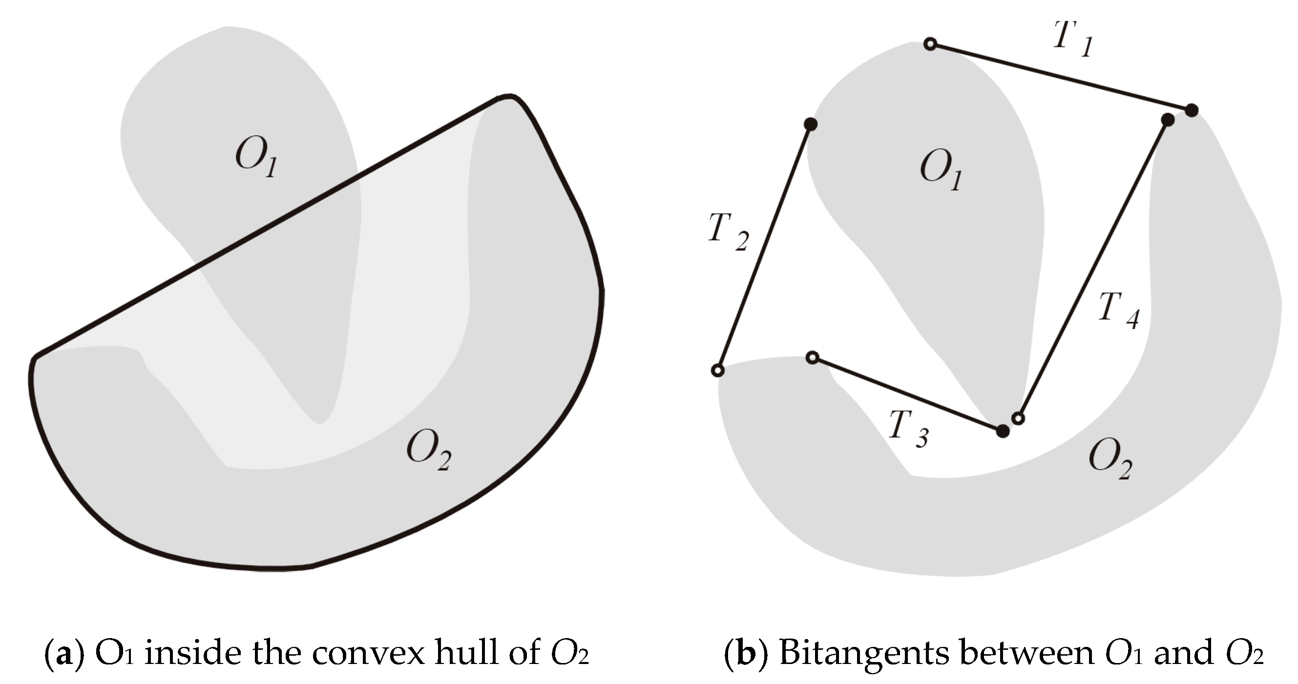
3.3. Eliminating Some Pointless Tangents

Shah and Gupta noted a possible simplification of the L-A graph that results from identifying some of the edges that cannot be part of the shortest path [28]. These are the edges that enter into the convex hull of another obstacle when this convex hull does not intersect any other obstacle or does not contain S or T. Figure 4 illustrates the situation: the lighter gray area represents the part of the convex hull of the obstacle that is not within the obstacle itself. The tangents AC and AD that end inside the convex hull, cannot be part of the shortest path as the end goal T is outside of it. Paths along these tangents would eventually have to come out of the convex hull, resulting in a longer path than one that directly bypassed the obstacle by going directly to points B or E.

Thus, it is critical to identify which of all tangents can possibly be part of the shortest path. We correspondingly define two classes of tangents, according to their topological properties. The first class consists of “obstacle glancing” tangents. These are rectilinear tangents that, upon arriving at a point P on the boundary of an obstacle and being prolonged past this point, never penetrate inside that obstacle. All of the tangents shown in Figure 5a and the tangents T₁ and T₂ in Figure 5b,c are glancing tangents. We let H_i represent the convex hull of the obstacle O_i.

The second class of tangents consists of the “obstacle penetrating” tangents. These are tangents that when prolonged past their point of contact with an obstacle O will penetrate inside of O farther. All of the tangents not identified as T₁ and T₂ in Figure 5b,c are such tangents. Such tangents may only appear in the shortest path to allow it to go through a passage between two obstacles. Figure 6 illustrates this situation: the three tangents shown are all obstacle penetrating tangents; however, they can be parts of a path segment that passes between O₁ and O₂. Such cases require special attention.

Shah and Gupta proposed to find the shortest path by using the A* algorithm with the visibility graph defined over quadtrees representing the terrain [28]. The consideration of quadtrees brings the simplification of reducing the shape of obstacles to assemblies of rectangles. However, the construction of quadtrees constitutes a preliminary step that requires appreciable computing resources. The method we propose bypasses the step of constructing a mathematical representation of the terrain by a quadtree or otherwise: it deals directly with a digital image of the landscape.

3.4. Our Definition of Simpler Graph Edges

The bitangents that link consecutive obstacles in the shortest path need to be connected together to make a continuous path. A new feature of our proposed method consists in doing this connection through a convex arc tangent to the obstacle boundary. Such convex arcs would be the paths that a bug-robot with an infinite range sensor would follow when moving under the Kamon et al. TangentBug algorithm [32]. They are the shortest paths that link two points on the surface of an obstacle. Figure 7 shows such a convex arc that links the two points A and B in the counter-clockwise direction.

Upon adopting the convention of Moravec, we characterize the direction in which a path follows the boundary of an obstacle, by virtually duplicating the obstacles and assigning a different direction to the boundaries of these duplicates. Thus, if O is the absolute value of the identity number of an obstacle, then +O and −O represent, respectively, the version this obstacle with the boundary in the counter-clockwise or in the clockwise direction. The notation O will stand for a signed obstacle number: either +O or −O.

The nodes of our graph are the starting point S, the destination point T and the points of arrival of the free rectilinear bitangents in the paths from S to T. The edges are made up of two connected segments: a convex arc that starts at a node on an obstacle and is tangent to its boundary, followed by a bitangent that extends from its end to another obstacle. Figure 8a shows a situation in which there are two edges: the segment ABC that links the two obstacles −O₁ and −O₂, and the segment ADE that links the obstacles −O₁ and +O₂. In Figure 8a, the parts of the convex hull of the obstacles, which are outside of the obstacles, are shown in pale grey. We note that that since +O and −O are considered as two different obstacles, there could well be an edge between them, as is the edge ABC in Figure 8b that links −O to +O. The graph so defined is actually a directed graph.

The graph so defined has a much smaller cardinality than the graphs of the L-A graph family. For example, it has only 8 nodes and 8 edges for the obstacles shown in Figure 3, while the L-A graphs have 18 nodes and 21 edges. This smaller cardinality implies that fewer steps will be required for the path optimization algorithm to construct the shortest path.

3.5. Adapting the A* Algorithm for Such Graphs

We remark that if all of the obstacles had disjointed convex hulls, as is the case in Figure 8a, then, a straightforward application of the A* algorithm would provide a solution to the shortest path problem. However, the general situation is more complex because part of some obstacles can lie inside the convex hull of other obstacles, as shown in Figure 5b,c and Figure 6. We recall that with the A* algorithm the whole graph does not have to be generated from the start; its nodes and edges can be simply generated when the computation process requires them. Thus, defining the graph construction process becomes an important inherent part of the algorithm.

3.5.1. The Notation

A path from the node n_i to the node n_k is an ordered set of nodes {n_i, n_i+1, ..., n_k} that are connected by edges, and that are traversed in the order in which they appear in this list. If an edge goes from the node n_i to the node n_k, then n_k is said to be a successor of n_i. n_m is said to be accessible from n_k if there exists a path from n_k to n_m. In our application, the cost c_ik assigned to the edge e_ik is simply the length of this edge. The cost of a path is the sum of the costs of all of its edges. A node is said to be expanded or closed when all of its successors have been generated. It is said to be an end node or an open node when none of its successors have been generated. In our adaptation of the A* algorithm, at any given time, a node will have either all of its successors generated or none of them generated. An obstacle O is said to be open when it has only some end nodes. It is said to be expanded when it has at least one expanded node. An evaluation function f is used to select the next node to be expanded in the algorithm. As is often done, we define f such that its value for the node n is

$$f\left(n\right)=g\left(S,n\right)+EDist(n,T),$$

(1)

in which $g\left(n_i,n_j\right)$ is the length of the shortest path in the graph, from the node n_i to the node n_j, and $EDist(n_i,n_j)$ is the Euclidean distance between n_i and n_j.

As pointed out by Moravec, some modifications are required in the standard A* algorithm in order to deal with the fact that the obstacles are not punctual so that many nodes can exist on the same obstacle. These modifications are described in the following sections.

3.5.2. Expanding a Node on an Open Obstacle

Expanding a node n on an obstacle O implies generating all of the edges that issue from that node. This involves determining all of the free rectilinear bitangents that leave obstacle O toward other obstacles and determining the convex arcs tangent to the boundary of O, which go from n to the point of departure of these tangents. When the convex arc and the bitangent do not intersect another obstacle, they correspond to an edge that starts at n.

Figure 9a illustrates a situation in which there are 5 end nodes, represented by black dots, on the boundary of the obstacle +O and numbered n_i, i = 1···5. Figure 9b illustrates the situation that results after one of these nodes, say n₅ for example, has been selected for expansion. The expanded node n₅ is outlined with a circle and all of the bitangents that leave +O are shown as rectilinear segments issuing from their point of contact, represented by a white dot. The edges that start at n₅ correspond to the tangent convex arcs n_5-a, n_5-b, n_5-c and n_5-d followed by the bitangents that start, respectively, at the points a, b, c and d. The bitangent that starts at e is not part of one of these edges because e cannot be reached from n₅ by a free tangent convex arc.

3.5.3. Expanding a Node on an Expanded Obstacle

Before describing this process, we prove a general theorem that brings an appreciable simplification to the application of the A* algorithm. Namely, it allows a disregard for the step that consists in remarking as open a node that was already marked as closed. We note that this theorem is valid for any graph in which the triangle inequality holds.

First-Node Theorem.

Once a node n_i has been expanded, it will never thereafter appear in a path from S that is shorter than its path from S at the time it was expanded.

Proof. 

Figure 10 represents the geometrical situation that corresponds to this theorem. In this drawing, the dashed lines represent paths that link two nodes in the graph, and the full lines represent rectilinear paths between two nodes. According to the A* algorithm, when a node n_i is expanded it is, at that time, the node with the smallest value of f. Thus, for every other node n, which had already been generated by A* and was still open,

$$f\left(n\right)\ge f\left(n_i\right)$$

(2)

If at some later time during the execution of the algorithm, the node n_i appears as a successor of n, then on the new path through n, {S, n, n_i} is such that:

$$f_{new}\left(n_i\right)=g\left(S,n\right)+g\left(n,n_i\right)+EDist(n_i,T)$$

but because of the triangle inequality

$$g\left(n,n_i\right)+EDist(n_i,T)\ge EDist(n,T)$$

$$\mathrm{s}\mathrm{u}\mathrm{c}\mathrm{h} \mathrm{t}\mathrm{h}\mathrm{a}\mathrm{t}\hspace{1em}{f}_{new}\left(n_i\right)\ge g\left(S,n\right)+EDist\left(n,T\right)=f\left(n\right)$$

(3)

then, from Equations (2) and (3),

$$f_{new}\left(n_i\right)\ge f\left(n_i\right)\mathrm{and}\mathrm{therefore}{g}_{new}\left(S,n_i\right)\ge g(S,n_i).$$

Thus, any path to n_i through n is necessarily not longer than the initial path to n_i, and could therefore be discarded from further processing in the shortest path construction.

□

We now describe the operations involved in the node expansion. Figure 11 illustrates the situation in which an end node x = n₂ on the obstacle +O, which is shown surrounded by a small circle, has to be expanded. The bare black dots are end nodes, the black dots surrounded by a small square are already expanded nodes, and the white dots represent the points of departure of some free bitangents. We denote by n the closest expanded node that precedes x on the obstacle boundary; this would be node n₅ in Figure 11. The IntegrateExpandedNode procedure, described hereafter, is then performed to expand node x.

• IntegrateExpandedNode Procedure

• If the nodes n and x can be connected by a free tangent convex arc on the boundary of O and

  $$g\left(S,n\right)+ConvexArcLength(n,x)\le g(S,x),$$

  (4)

  then discard node x because the path that consists of {S, n} followed by the tangent convex arc from n to x, is shorter than the path {S, x}. Terminate the procedure.
• Else, let m be the closest expanded node after x on the contour of O (this is n₃ in Figure 11).
• Then, for all of the points of the departure d_k of free tangents T_k, which lie between x and m and can be reached from x by a free tangent convex arc (which are the points b and c in Figure 11), define an edge that consists of the convex arc from x to d_k and the tangent T_k that leaves at d_k.
• Assign the node that corresponds to the point of arrival of the bitangent T_k on the other obstacle as a successor of x in the tangent graph.

The First-Node Theorem implies that the paths {S, x, y}, where y is any expanded node from m and further, will necessarily be longer than the already defined path {S, y}. Therefore, only the tangents that start before m can be assigned to an edge starting at x.

• End of the procedure.

3.6. Description of Our Adapted A* Algorithm

Recall that each obstacle is represented by the two integers: ±O according to the direction of travel on its boundary.

• Initialization:

Define S as an end node with f(S) = Edist(S,T).

Define the single points S and T as the obstacles +O_S and +O_T.

• Loop:

• Select for expansion the end node x that has the minimum value of f.
  Let O_x be the obstacle on which it resides.
• If O_x = +O_T then mark x and O_x as expanded and terminate the computation; a solution has been obtained.
• If O_x is expanded, execute the procedure IntegrateExpandedNode for x and go to Step 5.
• Mark O_x as expanded.
  Generate all of the edges that start at x.
  Mark all of the new nodes at the end of these edges as end nodes that are sons of x.
  Calculate f for each of these end nodes.
  If some of these end nodes are on unmarked obstacles, mark their obstacle as open.
• Mark x as expanded.
• Go to Step 1.

• End of the loop.

4. Details of the Implementation

We now explain how we realized this algorithm, as it is not evident how to proceed when performing only digital image manipulations instead of using mathematical constructs. In particular, we describe the preprocessing of the data, some small sub-algorithms that are the fundamental building blocks of the shortest path algorithm, the data representation that we used, and some pseudo-code that expands the succinct description of Section 3.6.

The data required for the algorithm is a digital 2D image of the terrain and the two points S and T. This image would typically be a photograph of the scene from above or a slice of a 3D digital surface model. This image is then binarized and segmented, which sets to 1 all of the pixels with a value above a prescribed threshold and sets the other ones to 0, which produces an image that we call the “Map”. The Matlab function “imbinarize” performs this task. The image Map can replace the image that has initially been provided in the computer memory since the latter is thereafter inutile.

Before running the algorithm, we can determine if a shortest free path exists between S and T. This can straightforwardly be done by labeling the blobs in the negative image of the Map, i.e., in not(Map), and checking whether the two points S and T belong to the same blob. If, and only if, they do there exists a path joining them. Obviously, if there are such paths, there exists a shortest path.

4.1. Preprocessing

The path construction algorithm requires the following data that are extracted from the Map.

• Identify the blobs in Map by writing in them an integer identity number and call the resulting image “etiquettes”. The Matlab function “bwlabel” can be used for this. Then, the Matlab function “regionprops” can provide the center of mass of these blobs. These are stored in a cell array called “centre”, such that centre{i} gives the 2D coordinates of the center of mass of blob “i”.
• Calculate the outside contour of each blob. This can be done by drawing a straight line from the corner of the image [1, 1] toward the center of mass of the selected blob, until this line hits the blob. Upon backing up to a neighboring pixel in free space, a walk is then performed on the outside contour of the obstacle in the positive direction around the obstacle. The list of N pixels so traveled is stored in a 2 × N cell-array we call “contour”.
• Calculate the list of the obstacles that have another obstacle penetrating into their convex hull. The non-overlapping of the bounding box of obstacles is an efficient first test to rule out such an occurrence. Calculating this list before running the algorithm saves having to check constantly during its execution whether obstacles are embedded in others.

4.2. Line Supercover Algorithm

This algorithm is the most fundamental tool in our implementation of the shortest path algorithm. It determines the list of all of the pixels that are traversed by a given straight line [33,34]. It differs from the Bresenham algorithm in that the latter determines only the pixels that will produce the appearance of a straight line in a computer rendition of an image [35]. The supercover algorithm is the one to use for determining whether or not a rectilinear path hits obstacles. Figure 12 illustrates the difference between the two algorithms; it shows, in gray, the pixels listed by each of these algorithms, for the same line.

4.3. Path Length Algorithm

We calculate the length of a path by traveling along it and counting one unit of length when moving from one pixel to the next one if they are on the same horizontal row or vertical column, and the length of $\sqrt{2}$ if they lie on a diagonal.

4.4. Obstacle Glancing Tangent Algorithm

Figure 13a shows the two shortest paths that go from point A into the shadowed region behind the obstacle. Their first segment is always a tangent from A to the contour of the obstacle, either one of the tangents T₁ or T₂. The tangent T₁ can be obtained as follows.

• Let B be any point on the contour of the obstacle as, for example, the point that is situated the farthest along the positive x-axis, as in Figure 13b.
• Find the pixel of the contour at which the angle BAC is maximum. The line AC is then the glancing tangent to the obstacle in the clockwise direction.

The glancing tangent T₂ is obtained similarly.

4.5. Bitangent Algorithm

Figure 14 illustrates a method for generating a bitangent between the two obstacles O₁ and O₂. Its steps are as follows:

• Select arbitrary points A and B, on the boundary of each of the obstacles. In Figure 14b, A is the farthest point along the negative x-axis for O₁ and B is the farthest point along the positive x-axis for O₂.
• Generate the glancing tangent AC from A to −O₂, as shown in Figure 14b.
• Generate the glancing tangent CD from C to +O₁, as shown in Figure 14c.
• Repeat Steps (2) and (3), while setting A = D and B = C, until the pixels of the arrival of the tangents on O₁ and O₂ remain unchanged.

Note that the complexity of this algorithm is essentially the same one as the secant method to find the zeros of a function, except that it is somewhat faster because the successive points in the construction are discrete integers.

4.6. Tangent Convex Arc Algorithm

This algorithm produces the list of the pixels that make up the smallest free convex arc that links two points A and B on the contour of an obstacle. This list is ordered in the anti-clockwise direction. Figure 15a shows such a path as a dotted black line. This convex arc is easily constructed as a boundary of the convex hull of the contour arc AB; the part of the convex hull that is not in the obstacle is shown in pale gray in Figure 15b. Convex hulls can be computed with any of the well-known algorithms.

4.7. Passage Entering Algorithm

This algorithm constructs a path that passes through the passage between two obstacles when one penetrates the convex hull of the other one, as shown in Figure 16a. The contour of the convex hull of the obstacle O₂ is shown as a thick black line and its interior is colored in pale gray. We note that there are somewhat more complex situations in which both obstacles have parts of them penetrating into each other’s convex hull. These cases can be dealt with in a similar manner as the present case. Figure 16b shows the four bitangents that connect these two obstacles.

The construction of a passage path, from left to right, is relatively straightforward when its starting point lies in one of the two regions illustrated in Figure 17a,b. Thus, when it starts at any point in the region shown in pale gray, in Figure 17a, the path can reach, tangentially, the boundary of O₂ in the clockwise direction. It can then follow a tangent convex arc on O₂ to reach the bitangent T₃ and then exit to the right between O₁ and O₂. Similarly, upon starting from any point in the region shown in pale gray, in Figure 17b, the path can reach, tangentially, the boundary of O₁ in the counter-clockwise direction, from which point it can follow the tangent convex arc on O₁ until it can leave the passage between O₁ and O₂.

The complication is that there is, in general, a particular region, shown in white and labeled as R in Figure 17c, from which the interior of the passage cannot be reached with glancing tangents to O₁ or O₂. The following procedure deals with this situation.

• Draw the glancing tangent from point A to obstacle −O₂, which arrives at point B, and the glancing tangent from A to +O₁, which arrives at point C. These two lines define the region o₂ in O₂, as shown darker in Figure 17c.
• Starting at A, construct the glancing tangent to −O₂, which arrives at point D on O₂.
• From this point, the path can follow the tangent convex arc in the clockwise direction on o₂ to reach the bitangent T₃ to get to point C, and proceed to exit through the passage. We then call the tangent from A to O₂ a passage entering tangent.

4.8. Data Representation

Before presenting the algorithm, we describe the nodes and obstacle structures that we use.

4.8.1. Node Structure

A node x of the graph will be represented by a structure with the following fields.

○

‘OnObst’: an integer that is the identification number of the obstacle on which the node resides.

○

‘Posn’: an integer that is the position of the node in the contour of the obstacle.

○

‘FromObst: the integer number of the obstacle from which x was reached.

○

‘g’: dist(S,x) = the shortest distance on the path so far determined from S to x.

○

‘f’: the lower estimate of the distance from S to T, while going through x.

○

OutTangents: the set of the structures that correspond to the tangents that leave this obstacle toward successor nodes of x on other obstacles, in increasing order of their starting position on the contour of the obstacle. These tangents constitute the last segments of the edges that start at x. The Tangent structures have the following fields.

○

‘FromPosn’: the position of the point of departure of the tangent in the contour of the obstacle.

○

‘ToObst’: the identification number of the successor obstacle, i.e., the obstacle to which the tangent in question is going.

○

‘ToPosn’: the position of arrival in the contour of the successor obstacle.

○

‘TanLength’: the length of the tangent.

A NodeId structure is used in some calculations instead of the whole node structure. It is defined with the following fields.

○

‘OnObst’: the number of the obstacle on which the node resides.

○

‘FromObst’: the number of the obstacle that is the father of that node.

○

‘f’: the same variable as defined in the node structure.

A set, called “ExpandedNodeIds”, contains the NodeId structures of all of the expanded nodes, and another set, called “EndNodeIds”, contains the NodeId structures of all of the end nodes already generated.

4.8.2. Obstacle Structure

For each encountered obstacle, we define a structure that contains all of the nodes that have been generated on that obstacle, at any instant of time. The set “ExpandedObsts” contains the structures of the expanded nodes and the set “EndObsts” contains those of the end nodes that are not yet expanded.

The obstacle structure has the following four fields.

• ‘ObstNo’: the integer identification number of the obstacle.
• ‘EndNodes’: the set of the structures that represent the nodes without successors that reside on this obstacle, in the increasing order of their position in the contour of the obstacle.
• ‘ExpandedNodes’: a similar set as the preceding one for the nodes that have been expanded.
• ‘FreeTangents’: the set of tangent structures that represent the tangents leaving this obstacle toward other obstacles, while they have not yet been assigned to a node on this obstacle.

Obst(x) will denote the obstacle structure for the obstacle on which resides the node x. Note that all of the nodes on expanded obstacles are not necessarily expanded, but all of the nodes on end obstacles are necessarily end nodes.

A set called ObstNos contains all of the obstacle numbers. When there are N obstacles, the obstacle number N + 1 is assigned to the starting point S and N + 2 to the target point T.

4.8.3. The Algorithm Pseudo-Code

• Initialization:

• Set Node(S)’s properties:

OnObst = N + 1	Posn = 1	FromObst = 0,	TanLength = 0
g = 0	f = Edist(S,T)	OutTangents =ϕ

• Set NodeId(S)’s properties: OnObst = N + 1, FromObst = 0, f = Edist(S, T)
• Set Obst(S)’s properties:

ObstNo = N + 1

EndNodes = {Node(S)}

ExpandedNodes = ϕ

FreeTangents = ϕ

• Set EndNodeIds = {NodeId(S)}
• Set ExpandedNodeIds = ϕ
• Set EndObsts = {Obst(S)}
• Set ExpandedObsts = ϕ
• Set ObstNos = {1, 2, ..., N, N + 2, −1, −2, ..., −N}
• Computation Steps

(1)

Select for expansion the node x that has the minimum f and denote by NoObstx its obstacle number.

(2)

If NoObstx = N + 2 then mark x and Obst(x) as expanded and terminate the computation.

(3)

If Obst(x) is expanded, execute the IntegrateExpandedNode procedure and go to Step 5.

• For all obstacle numbers NoObsty in ObstNos that differ from NoObstx,

compute the bitangents as follows:

• If Obst(x) has no embeddings from Obst(y) and Obst(y) has no embeddings from Obst(x),
• compute the simple bitangent Tan(x,y) between the two obstacles x and y.
• If Obst(x) has no embeddings from Obst(y) and Obst(y) has embeddings from Obst(x),
• execute the PassageEnteringAlgorithm and let Tan(x,y) denote the passage entering tangent.
• If Obst(x) has embeddings from Obst(y) and Obst(y) has embeddings from Obst(x),
• compute the set TanL(x,y) of all of the mutual tangents.
• If Obst(x) has embeddings from Obst(y) and Obst(y) has no embeddings from Obst(x),
• compute the simple bitangent Tan(x,y) between the obstacles NoObstx and NoObsty.

Incorporate the bitangents as follows:

• for Tan(x,y) or each element Tan(x,y) in the set TanL(x,y):
• If Tan(x,y) is not free, then continue.
• Otherwise, compute the tangent convex arc ConvexArc on Obst(x) that starts at the position of x and ends at the leaving position of Tan(x,y) on Obst(x).
• If ConvexArc is not free, then put Tan(x,y) into the FreeTangents set of Obst(x) to be dealt with later on, and continue.

Otherwise, set gy = x.g + length of ConvexArc + length of Tan(x,y);

set fy = gy + EDist(y, T);

define Node(y) with the following parameters

OnObst = NoObsty	Posn = Tan(x,y).ToPosn	FromObst = NoObstx
TanLength = Tan(x,y).TanLength	g =gy	f =fy	OutTangents =ϕ

• If the structure for Obst(y) does not already exist,
• define it with the following properties:

ObstNo = ObstNo

EndNodes = {Node(y)}

ExpandedNodes = ϕ

FreeTangents = ϕ

• Mark it as an end obstacle.
• Otherwise, add y to the Obst(y) set of EndNodes.
• Insert Tan(x,y) into the OutTangents set of node x.

• End of the loop: “For all obstacle numbers”.

(4)

If Obst(x) was not an expanded obstacle,

mark it as expanded and unmark it as an end node.

If it has not been discarded at Step (3), mark it as expanded.

(5)

Go to Step 1.

• End of computation.

Once the algorithm has been run, the shortest path can be read backward, starting with the end node T and following the successive father nodes, until node S is reached.

5. Some Remarks on the Complexity

Analyzing the complexity of our proposed refined A* search algorithm, combined with our new theorem, is a formidable task in itself that we should undertake in a separate study. It is intuitively clear, however, that, since a step of the A* algorithm is eliminated, our algorithm should be better than the standard version of the A* algorithm. For the moment, we will simply recall some general facts about an upper bound for its complexity. The fact that it is realized with graphical manipulations on a digital image does not increase its complexity. Shah and Gupta who used a standard A* with a quadtree representation of the terrain, mentioned that the complexity of their method is only marginally affected by the number of pixels in the images [28]. Both the graph construction and the A* calculations remain the same whatever the number of pixels because these depend only on the nature of the distribution of the obstacles. They mentioned expecting the contribution of the number of pixels to the complexity to be of O(n), where n is the density of pixels. This is also the complexity given by Andrew and Dedu for the line supercover algorithm that we use constantly in our algorithm to trace the straight-lines [33,34].

Given the important similarity between the A* algorithm and Dijkstra’s algorithm, Rachmawati and Gustin undertook to compare them for solving the shortest path problem [36]. They found “the only difference being that A* tries to look for a better path by using a heuristic function, which gives priority to nodes that are supposed to be better than others while Dijkstra’s just explore all possible ways”. A* scans the terrain preferably in the direction of the destination, whereas Dijkstra searches equally in all directions. Thus, the latter ends up exploring a much larger area before the target is found, making it slower than A*, although no one has yet quantized this difference. They mention that this advantage can be demonstrated by the loop count of Dijkstra and A*; the more nodes there are, the higher the difference between the loop counts will be.

They actually then performed some tests with a network of 101 road intersections in a Google map of the vicinity of the city of Kota Matsum in Indonesia. They counted both the number of loops and the execution times for the same shortest path problems with the A* and the Dijkstra algorithm. They found that the loop count of the A* algorithm was indeed consistently smaller than that of Dijkstra’s algorithm, even for small numbers of nodes. For small problems, the execution times of both were similar. However, for large problems, with about 100 nodes, the loop count of A* was about three-quarters that of the Dijkstra, and its execution time was about one-quarter smaller.

Chang et al. examined the complexity of bitangent algorithms to solve the shortest path problem for a terrain with disk obstacles [23], in which the nodes and edges are defined as described by Moravec. Given that the core of our approach is essentially the same one as that of Moravec, except for the shape of the obstacles, we do not expect our algorithm to differ very much in complexity from his. The authors note that when there are N disks, there are then O(N²) nodes and O(N²) edges. Most shortest path algorithms are some version of Dijkstra’s algorithm for which the length of the edges is their weight. They remarked that, for a graph with V nodes and E edges, Dijkstra’s algorithm can be implemented to run in O(E + V logV) = O(N² logN) time. Therefore, the complexity of the A* algorithm is bounded above by this expression.

A final remark about the storage memory space used by our proposed method is worthwhile. The input data is a digital image that is read in the computer memory. This image is then replaced by the image of the labeled blobs (the “etiquettes” image). The contour of the obstacles can be painted in this image, thus not requiring any additional memory space. Therefore, the permanent data on which the algorithm works takes essentially the same amount of memory space as the initial digital image.

The main task performed by our algorithm, is the calculation of rectilinear tangents; we note that once they have been calculated, only their end points are stored in memory. When convex tangent arcs are calculated, they are immediately tested to see if they are free or not, and are thereafter not kept in memory. The data stored in the structures, created by the algorithm, themselves consist only in a few integer numbers and most calculations with pixels involve only integers.

6. Results

We now present examples of the shortest paths generation by our method for some real-world digital elevation maps (DEM), and for one artificial landscape with forbidden zones. These maps represent various regions of the world that were used as examples in [1]. The altitude of the UAV at which the trajectories lie has been set to some plausible values. The paths obtained are shown in Figure 12. The computations for each example were done with our implementation of the algorithm with the software Matlab 2020b and run on a portable Omen laptop from HP with an Intel Core i7-10750H CPU @ 2.60GHz. Details on this CPU are given in Appendix A. The computation times reported are the averages of 10 runs of the same calculation of the solution.

• Artificial canyon

The map of Figure 18a represents a fictitious terrain. Its dimensions are 500 × 500 pixels, and the size of the terrain is 5 km × 5 km. To this terrain, we have added four circular no-fly zones. The landscape shown corresponds to a plane at an altitude of 100 m. The starting position is [10, 250]^T and the target position is [400, 250]^T. The length of the shortest path is 4799.2 m. The calculation requires 0.1125 s.

• Austrian Alps

The map in Figure 18b represents the terrain in the Austrian Alps, with the town of Imst to the west and Telf to the east. It has 385 × 500 pixels and represents a region of 30 km × 39 km at an altitude of 1700 m. S = [25, 40]^T and T = [350, 90]^T. Note that the path correctly goes through the passage at the start of the trajectory, in the upper left hand side corner of the map. The length of the shortest path is 36,825 m. The calculation requires 0.1732 s.

• Canadian Rockies

The map in Figure 18c represents the terrain through which flows the Fraser River near Lillooet, BC, Canada. It has 419 × 500 pixels that correspond to a region of 8.7 km × 10.4 km. The path is in a plane at 450 m of altitude with S = [50, 400]^T and T = [350, 150]^T. The length of the shortest path is 12,354 m. The calculation requires 0.0793 s.

• Norilsk, Russia

The map in Figure 18d represents the terrain east of Norilsk in Russia. It has 416 × 500 pixels that correspond to a region of 24.4 km × 29.3 km. The path is in a plane at 600 m of altitude with S = [175, 75]^T and T = [375, 325]^T. The length of the shortest path is 27,265 m. The calculation requires 0.0621 s.

• Lima, Peru

The map in Figure 18e represents a region around Lima, Peru. It has 380 × 500 pixels that correspond to a terrain of 15.5 km × 20.4 km. The path is in a plane at 500 m of altitude, with S = [195, 45]^T and T = [50, 470]^T. The length of the shortest path is 25,061 m. The calculation requires 0.5501 s.

• Grand Canyon, USA

The map in Figure 18f represents a region around the Grand Canyon in Colorado, USA. It has 332 × 500 pixels that correspond to a terrain of 4.9 km × 7.3 km. The path is in a plane at 100 m of altitude with S = [190, 495]^T and T = [190, 75]^T. The length of the shortest path is 9416 m. The calculation requires 0.1141 s.

7. Discussion

We have proposed a new method for the construction of the shortest path through a 2D field of obstacles of arbitrary shapes and positions. The novelty of this method resides in part in the definition of a new type of graph that is simpler than previously considered graphs in that its edges are a concatenation of many edges and nodes defined in previously used graphs, such as those of Liu and Arimoto. Thus, this lower cardinality of our graphs evidently reduces the required calculations. Furthermore, our topological analysis of the obstacles revealed that many path segments can be discarded because they can actually never be part of the shortest paths.

In this work, we present a new theorem, which we have discovered, that allows us to disregard one of the steps that is normally performed in the A* algorithm; this theorem applies for all graphs in which the triangle inequality holds. We subsequently described a new variant of the A* algorithm that generates the shortest path, based on this theorem and our graph definition.

The efficiency of our method is demonstrated by the construction of the shortest path for some real-world terrains that correspond to mountainous regions, represented by digital elevation maps. The computation times for these examples, on a small laptop, are seen to be less than 0.6 s in all cases.

8. Conclusions

We have proposed a new algorithm for the construction of the shortest path through a 2D field of obstacles of arbitrary shapes and positions. This algorithm has the important rare advantage of not requiring the preliminary construction of mathematical expressions to represent the obstacles, such as quadtrees or others. It operates directly on a digital map of the terrain without requiring the construction of any mathematical representation of the obstacles. Its implementation requires solely standard digital image processing functions. It can be realized on essentially any computer, because it does not require large amounts of memory or computing power. It can deal with generic terrains, whatever the shapes of the obstacles and their distribution in space. Some examples have been provided of its working with some real-world digital elevation maps.

It would be worthwhile to make a future study to compare the behavior of the standard Dijkstra algorithm and that of our proposed algorithm, in solving the same problems. Such a study would be along the lines of Rachmawati and Gustin who obtained some definite results when comparing the Dijkstra with the standard A* on a set of shortest path problems.

Given the rapidity of the solution process, this algorithm can be used in real-time, on-board the vehicle, when updates to the mission terrain are received. Thus, future work will consider constructing shortest paths when some of the obstacles are moving. A future non-trivial challenge will be to adapt this algorithm so that it takes into account the existence of a minimum turning radius, which most vehicles have, such as airplanes, ships, and automobiles. Indeed, as constructed by the present algorithm, most shortest paths will have some sharp corners as they graze the boundary of angular obstacles. Further work should follow on this subject.