Abstract
Tensor networks are a very powerful data structure tool originating from simulations of quantum systems. In recent years, they have seen increased use in machine learning, mostly in trainings with gradient-based techniques, due to their flexibility and performance achieved by exploiting hardware acceleration. As ansatzes, tensor networks can be used with flexible geometries, and it is known that for highly regular ones, their dimensionality has a large impact on performance and representation power. For heterogeneous structures, however, these effects are not completely characterized. In this article, we train tensor networks with different geometries to encode a random quantum state, and see that densely connected structures achieve better infidelities than more sparse structures, with higher success rates and less time. Additionally, we give some general insight on how to improve the memory requirements of these sparse structures and the impact of such improvement on the trainings. Finally, as we use HPC resources for the calculations, we discuss the requirements for this approach and showcase performance improvements with GPU acceleration on a last-generation supercomputer.
1. Introduction
Tensor networks (TNs) provide a characterization of quantum states with a connection to physical states of local Hamiltonians [1] that may be efficiently represented classically. They have become an indispensable tool in the field of simulating quantum systems, as they offer highly developed methods that are parallelizable for large-scale computations. For example, they are used for circuit simulation [2] with large network contraction heuristics [3] or using a state vector with bounded bond dimension [4], and in condensed matter computations with 1D [5] and higher-dimensional methods [6,7]. These computations with classical tools push the frontier of experiments that require simulation with quantum resources [8]. In fact, they have recently played a role disproving quantum advantage claims [9] in cutting-edge Noisy Intermediate-Scale Quantum devices [10].
A particular type of 1D TN, namely Matrix Product States (MPSs) [11], has been identified as the variational structure operated by the celebrated Density Matrix Renormalization Group algorithm (DMRG) [12]. Moreover, their flexibility in storing data and the usefulness of the bond dimension , a parameter that controls how much correlation is allowed, has enabled this tool to see success in machine learning as well [13,14] using gradient-based tools (either first- or second-order), similarly to classical machine learning. Other regular structures, such as 2D projected entangled pair states (PEPSs) [7] or the multi-scale entanglement renormalization ansatz (MERA) [6], have also been extensively used for successfully simulating many-body systems.
The choice of the TN geometry is related to how physical systems present different entanglement structures: networks with high complexity might be able to represent interesting states better. On the other hand, the use of highly intricate TN structures is limited by the computational cost of contractions and increased memory requirements. The interplay between these behaviors is crucial when choosing the strategy to solve a problem, and a common and reasonable approach is to settle for one of these regular structures that is just complex enough for the target system, but not more [15]. Another option is to find heterogeneous geometries that are tailored to the target system, which has seen growing interest recently, with proposals to characterize them mathematically [16,17], as well as algorithms to find the optimal choice [18,19,20]. The geometric traits used in these descriptions and algorithms have an impact on the training performance in real applications, but have not been characterized, despite their relevance in contraction strategies [3], numerical implementations [21], large-scale computations [22], and the appearance of barren plateaus [23,24].
In this article, we present different low-dimensional TN structures and characterize them in terms of contraction costs and memory usage. We train them to copy random quantum states, which do not have any implicit correlation structure, using a set-up that relies on gradient-based tools with automatic differentiation. To do so, we propose a tensor contraction with a surrogate tensor, which gives us complete control over the complexity of the target system and avoids some statistical subtleties of training with samples. This enables the establishment of a training method much more suitable for testing different properties of heterogeneous TNs with systems of specific geometries. In addition, we introduce the compact version of any tree TN structure and discuss when it can present an advantage. These simulations reveal links between the quality of the encoding and the density of these heterogeneous TN structures, as MPSs and some large-diameter tree TNs perform worse than their more dense counterparts, even though the bond dimension is high enough to store the same amount of information in principle. We also include some trainings with target systems of reduced complexity, offering numerical evidence for the advantage of these compact tensor networks and further support regarding the impact of density.
Any of the aforementioned TN uses are of special interest in large simulations with high-performance computing (HPC), as their performance outshines cruder methods at that scale. Improving the time and energy efficiency of computations is a principal aspect of this field, as it extends the range of feasible simulations. In recent years, GPU acceleration has become crucial for performance improvements [25], and has in fact been integrated into the latest-generation Marenostrum 5 supercomputer. The training presented in this work was built on libraries that allow us to compare performance with and without acceleration. For these reasons, our results include a comparison between CPU-only nodes and GPU-accelerated nodes that shows an advantage in performance for large enough systems.
Dynamically looking for optimal heterogeneous geometries is a promising avenue for increasing the strength of TNs in simulation, and heuristic solvers can especially benefit from our findings on the importance of density and the effect of compactification, which had not been studied yet. Similarly, understanding what properties matter the most in the quality of the approximation can help understand machine learning solvers too. We conjecture that this behavior is strongly related to the interplay between data distribution in the structure and training methods, suggesting that DMRG and other TN native methods would also benefit from a TN structure imitating that of the target state. On the other hand, our proposed surrogate training approach enables the design of further experiments in this direction, by allowing us to match any structure in the model with varied TN structures in the learning procedure. We recommend viewing all plots in this article in color to properly distinguish the data for each TN geometry.
2. Tensor Network Structure
2.1. Bond Dimension and Correlations
Entanglement is a crucial property of quantum systems that distinguishes them from systems with only classical properties [26]. It is related to the correlations between different parts of the system, and while it has been extensively studied in the case of bipartitions, characterizing and quantifying multipartite entanglement in general is still a profoundly complex topic [27,28]. For a quantum state with density matrix , subsystems A and B of a physical state are not entangled (and are thus completely uncorrelated) when they can be written down as a tensor product [29]. Otherwise, this decomposition requires a sum of different product states, and A exhibits entanglement with B. This can be related to the Schmidt decomposition of a quantum state [29], which for a bipartition is also
When looking for the tensor product decomposition on of the density matrix of such a state, , it is clear that the number of terms in the Schmidt decomposition dictates how many tensor product terms are needed. We call the number of states needed in this sum the Schmidt number . Sometimes, we do not need many elements in the decomposition, so is small, which can happen, for example, when the entanglement between A and B is small.
Tensor networks [30] can encode high-dimensional tensors into the product of smaller, low-dimensional ones. This can be generally useful for data encoding [31,32] in the classical setting, where they are sometimes known as tensor trains [33], although they are more commonly used in the simulation of quantum systems [15]. In the quantum setting, the high-dimensional tensor is commonly a quantum state of n sites, which, before decomposing, needs to store coefficients, with d representing the dimensionality of each site. For example, quantum digital computing uses qubits with . Such decomposition is advantageous whenever correlations between tensors that are far apart in the network are not too high, as it means that those sites present a small amount of entanglement. Then, a bipartition separating these tensors, following Equation (1), does not need a large dimension to encode the full state, and the sum of memory required by all the small tensors can be smaller than that required by the large, contracted tensor. The low-dimensional tensors can be connected through bonds in various geometries, which can be useful depending on the entanglement structure of the system they encode, although networks with more complexity and expressive power will entail higher performance costs.
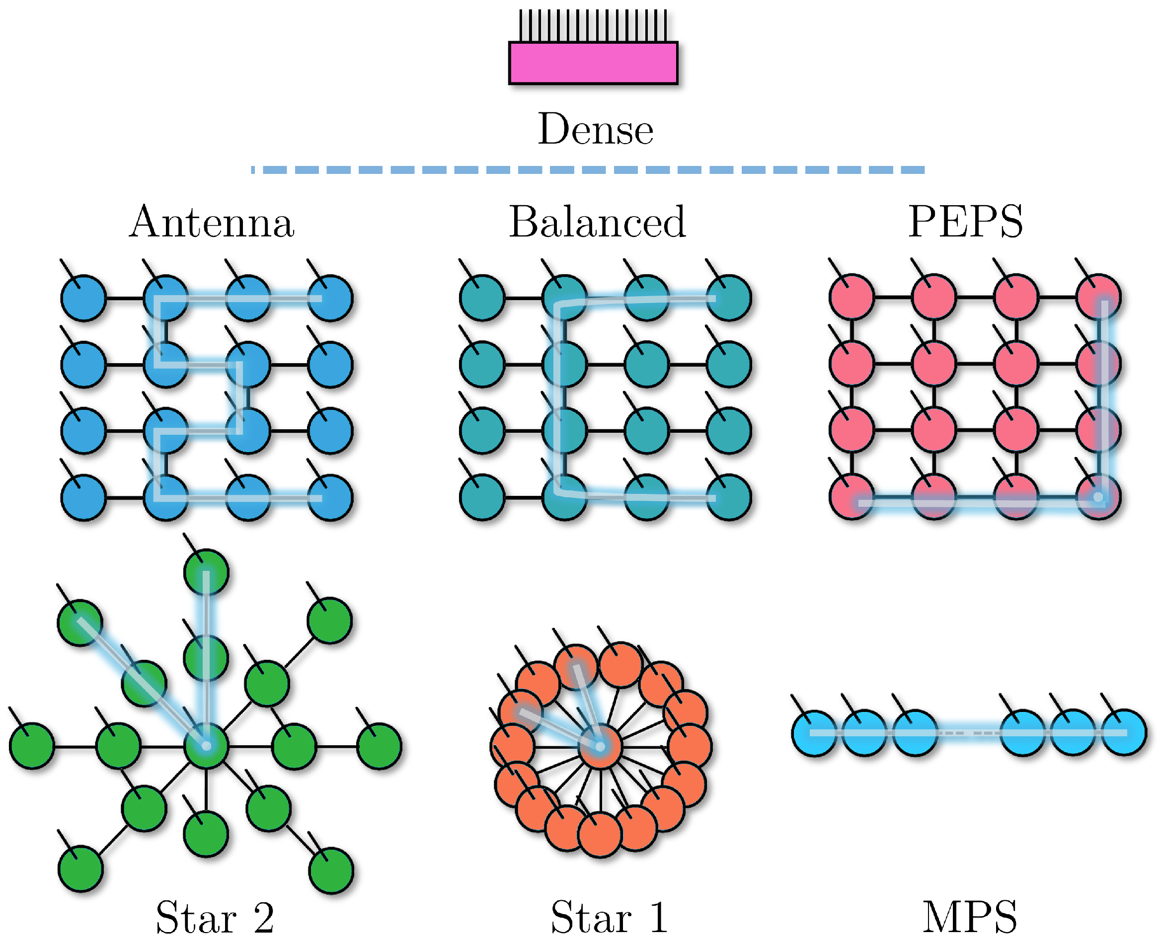
One of the advantages of tensor networks is the flexibility of their graphic notation. Each tensor is represented by a small node, usually round-shaped, and the bonds between tensors are lines that connect these nodes. These are called virtual bonds, or virtual indices, as they depend on the geometry of the tensor network and not necessarily the properties of the system they encode. If their dimension is as large as the Schmidt number for the bipartition of the two parts of the system they connect, the tensor network is a faithful encoding of the system. We denote the maximum of the dimensions among all virtual bonds as the bond dimension . The dimension of the system, on the other hand, is encoded in the physical bonds (indices), which are connected to a node on one side and free on the other. A few examples can be seen in Figure 1. The original high-dimensional tensor can be recovered by contracting all virtual bonds.
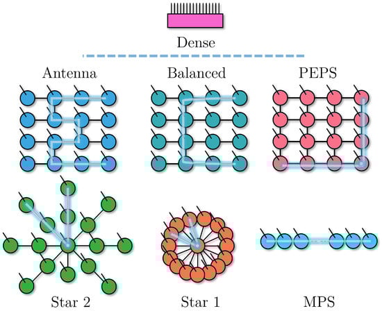
Figure 1.
The TN geometries used in this work, with a few tree-like TNs (including an MPS) and the PEPS ansatz. The highlight indicates the longest path between tensors, which we use as a measure of density. For the PEPS, instead, it shows the longest minimal path between nodes when considering all node combinations. At the top is a single tensor equivalent to the contraction of any of the other geometries.
A tensor network diagram is directly equivalent to an equation between the original tensor and the small tensors, which makes the contractions explicit. We use an MPS [30] example to illustrate this, which is a 1-dimensional chain and thus the simplest example of a non-trivial tensor network. Here, the high-dimensional tensor T with n physical bonds is equivalent to the contraction of n tensors as follows:
It is possible to see in this example how the bond dimension is linked to the entanglement properties of physical systems. For a separable state, any bipartition will have , so it can be encoded into a TN with . Other states can have entanglement limited to a 1D nearest-neighbor, such as the AKLT state [34], which needs . A maximally entangled state requires up to , which is in fact the upper bound of for any system of n qubits, so an MPS with this can represent any state with perfect precision. Beyond these exact cases, the bond dimension can also be reduced at the cost of precision. For example, even if a bipartition on a state has a large , it can still be that most of the coefficients are very small, which is equivalent to low entropy S across that bipartition. Then, a tensor network with can encode an approximate state that is almost identical to the original in terms of the fidelity .
Efficient simulations with tensor networks rely on limited entanglement, mostly between close neighbors [1], or on a hierarchical structure of entanglement [6,35]. In the extreme case of no entanglement, the simulation cost of a system grows linearly with its size; in more complex cases, systems can adhere to an area law [36] that allows TN methods like DMRG [5] to perform efficient simulations with great success. Precisely because bond dimension makes entanglement and correlations in general both visible and accessible, tensor networks are very useful as a tool to understand quantum states, phases, and algorithms [15]. When we find that a quantum family of states can be simulated with a TN ansatz, we obtain a great deal of information about its correlation structure, and we can deduce that a system presents linear entanglement, area law entanglement, etc. Conversely, if we find a system with these properties, we know that TN ansatzes are a good fit for simulation.
2.2. Choice of Structures
We focus our study of gradient-based tensor network training mostly on different tree tensor networks, also including the 2D PEPS [7] geometry comparison when the size of the system allows it. In Figure 1, we show each different geometry used in the training. Beyond the known ansatzes of MPSs and PEPSs, we have an “Antenna” structure that reduces the distance between sites with respect to an MPS, without allowing tensors with more than three virtual indices, whereas “Balanced” achieves an even smaller distance at the cost of having bigger tensors with four virtual indices. We also propose a highly connected tree with “Starn”, where a single site is connected to many sites. For , the site distance is minimal without introducing loops, and the central tensor is as complex as the dense tensor, but the contractions of tensors on a single site are minimally expensive (comparable to the edge of an MPS). As n grows, the beams of the star have more nodes and the distance between nodes increases. In the trainings, we use (despite not being depicted in Figure 1), and especially require much bigger tensors than the other tree structures.
Tree tensor networks have traditionally been used with the binary tree structure [37], which was also a precursor to the success of MERA [6]. This structure can be made more flexible by dropping the binary requirement [38]. The structures that we study here are equivalent to this generalized tree TN but with some of the branches contracted. One can also allow for loops in the connectivity, which increases the representation power of the structure, but has to forgo most of the performance in the algorithms that make MPSs very efficient (for example, using canonical tensors becomes much more complicated [39,40]). The connectivity of the structure, once loops are allowed, can be taken beyond 1D MPSs and 2D PEPSs into the extreme all-to-all case, in which an n-site system would be encoded into an n-dimensional tensor network, reaching maximal contraction complexity and representation power. On the other hand, restricting the ansatz to be loop-free makes it possible to establish an ordering inside the structure, which allows MPS tools to be used while still making use of the increased flexibility beyond a chain structure [37].
Heterogeneous TNs such as the irregular trees we study here are not very commonly used. A structure that works well in general and has highly developed tools can present good performance for optimizing a systems that is not characterized, even if it is not optimal. However, an efficient heuristic that tailors a structure to a given problem could offer an additional advantage. Efforts in this direction have recently been made, both with intuitive heuristics [20] and with machine learning methods [18,19], achieving good results in terms of identifying entanglement structures in a specific system [41]. These structures are thus a good fit for systems whose known properties picture a certain entanglement structure, from which one can propose a physically motivated ansatz. We contribute to this application by studying the benefits and drawbacks of the resulting structures in regard to training methods. In the future, these experimental findings can help bridge the field with research that aims to characterize TN geometries mathematically [16,17].
2.3. Training with a Surrogate System
Training a model in machine learning usually requires a large number of samples [42] which contain the information that we want to learn. Thus, one can expect a training to consist of a set of k samples , which are extracted from a target physical system, and a model [43], which is expected to generalize well following some known properties or theorems. In the setting of using tensor networks as the model , this translates to a contraction between samples and the TN ansatz, which is commonly a simple MPS [13] or a similar structure [14]. These contractions are accounted for as an ensemble in some appropriate cost function . Such an approach must deal with issues like generalization of the model, sampling complexity, and so on, which are quite complex [44] and depend not only on the structure of the TN ansatz but also the training set and the properties of the model we are trying to learn.
We propose training with a surrogate TN that represents the physical system directly in a single tensor, avoiding some of these learning issues. With this method, depicted in Figure 2, we can prepare physical systems that have specific entanglement structures or limited correlations and study how well they can be learned for a given geometry. This is achieved by initializing a random tensor network with the structure ansatz we are interested in, fixing , and then contracting it into a single tensor. In the final state vector-like form, the surrogate hides its origin, as would happen for a target physical system with unknown properties. Because we have to prepare the tensor, it is not a substitute for learning unknown systems, but rather, a useful tool for controlled experiments. Instead of many contractions with each sample , we perform a single contraction between the surrogate and the model which avoids the statistical problems of sampling but, on the other hand, is more costly computationally. The final trained model in the ideal case of perfect training should be equivalent to the physical system itself, and since the model has a TN form, it is then equivalent to the surrogate itself. In this work, we focus on controlling the complexity of the target system (which would extend to that of the samples) via the bond dimension of the surrogate for two different scenarios, as we will explain in Section 3, and leave for future work the study of encoding different structures into the surrogate to see if we can recover them.
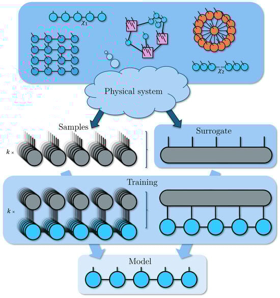
Figure 2.
The usual training process of a TN model using samples of a target unknown physical system, to the left, compared to our method with a surrogate TN, and to the right, where we control the number of correlations in a TN with its bond dimension, and then we contract it into a single dense tensor. Both approaches output a model of the physical system in the form of another TN (in the example, an MPS).
The structure of the TN model plays a crucial role in several ways. It directly constrains how hard it is, computationally, to contract the network. Consequently, it also characterizes how hard it is to find the optimal path for such contraction, with an MPS on one end (the optimal path is known beforehand) and the contraction of non-structured tensor networks, like in arbitrary quantum circuits, [3] on the other (known heuristics can find good paths, but not optimal). It also relates to how well they can represent the system that is being encoded in them. This is an obstacle that can be overcome with enough resources, as we have seen that without binding , even an MPS could represent the most complex quantum state. However, we will see that even with large , wide geometries that have enough correlations between sites can still fail to train properly. More generally, finding the appropriate geometry that reflects the correlations between different parts of the target quantum system can keep bond dimension costs and, thus, the computational cost lower, but such benefits must compete with how easy it is to find and train them.
2.4. Tensor Budget
In the design of our tensor network, it is important to budget the resources properly. Memory limitations are very relevant to the size of simulations that can be achieved [45,46], and common strategies to improve performance involve a tradeoff between memory and computational cost, especially in the HPC setting [47]. This tradeoff has a direct equivalent in tensor networks. In an MPS with a fixed bond dimension , for example, we can contract all sites with a virtual index smaller than without losing information or correlations. This is evident when using the maximum : for an odd n-qubit system, the central tensor with one physical bond and two virtual bonds has the same dimension () as a dense representation of the same quantum system (). On the other hand, each contraction on these redundant sites becomes more expensive, which is relevant for Time-Evolution Block Decimation (TEBD) [48,49] or circuit simulation [46], as depicted in Figure 3. This method can be trivially generalized to any TN structure without a loop. Such structures employ more tensors than strictly necessary for the amount of information that they store; from another point of view, the information is distributed over a larger number of variables that need to be trained.
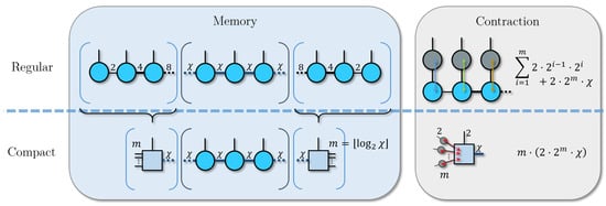
Figure 3.
Example using an MPS of the “compact” TN approach, where bonds smaller than are contracted. This reduces the memory needed to store the tensor network, but increases the cost of the contraction for the compacted sites.
We can show explicitly when this contraction effect is relevant in the MPS. For a given , and assuming that the physical indices have a fixed dimension p, let us consider two tensors that share a bond with dimension . The tensor that is further from the center of the MPS has a left virtual index of dimensions of at most , so in total, it needs a memory of at most , whereas the other tensor needs , where is its other virtual bond. The contracted tensor then occupies a memory of , which is the same as the second tensor. Thus, the sum of both uncontracted tensors will always be strictly larger. Starting from one end of the MPS, if we carry out this process m times before reaching the tensor with virtual bond dimension , we will have a tensor with dimensions . Therefore, m is the largest integer smaller than . In particular, for the usual case where , we have . We can repeat this process from each end of the MPS.
The closed formula for the MPS case cannot be generalized to arbitrary tree TNs, as it depends on the branching structure, but we can apply the same concept to decide which tensors to contract. Considering the leaves of the tree to be the tensors, with only one physical bond and one virtual bond, we start contracting the branches until we reach a tensor with a bond of size . For tree tensor networks with few branches (or where most branches connect to few tensors) the effect will be similar to that of an MPS, whereas for many branches, the memory reduction will be much more substantial.
This effect of compactification is rarely the leading performance or memory factor in large MPS simulations, since that depends on the large tensors that are far from the endpoints (leaves) of the network. Specifically, it is negligible when . Regardless, it can be used to increase the quality of the results that are achievable with a fixed memory budget, especially with low bond dimensions or sites. On the other hand, tree structures can benefit much more, namely those with a small average distance between nodes, as they have a larger number of leaves. If the distance is too short or the bond dimension too large, this scheme naturally outputs a single dense tensor (i.e., the state vector, for quantum systems). This only happens when the resources are high enough to compute the whole system, in which case, training the dense tensor is indeed the optimal approach when the target has close to maximal complexity, as we show in this article. To quantify the effect of this modification at a practical level, we use a target system with reduced complexity and train a compact version of each tree structure, as shown in Figure 1. This way, we can achieve good simulations with a smaller bond dimension and see the effects of this technique without all compact TNs being equivalent to the dense tensor. As in the rest of the simulations, we study the training in terms of time, contraction cost, and memory usage.
2.5. Barren Plateaus
Barren plateaus are an obstacle in the training of current quantum variational algorithms [50], and their existence has recently been linked to simulability [51] for all known trainable instances, supporting previous suggestions of a structural rethinking in the current search for quantum advantage in quantum machine learning [52]. In the study of TNs for computation, however, this outlook plays an opposite role. It motivates the exploitation and improvement of TNs with quantum algorithms to define the limit of quantum advantage by pushing the boundary of simulation techniques.
This problem extends to the training of tensor networks, as has been shown in the last few years [24]. The structure of the TN in use greatly affects the appearance of plateaus [23,53], with MPSs being the most susceptible. This effect should be considered together with our findings on memory, efficiency, and precision when judging our conclusions on the suitability between structures and training applications. In fact, for certain sizes of the system, we encounter them in our training of the MPS despite being absent for the denser geometries, as we will show in the Section 4. While this is consistent with previous findings, the progressive improvement in success rate as the density increases shows that there is not a categorical distinction between the MPS and the rest of the structures; instead, there is a somewhat continuous correlation between the complexity of the TN and the appearance of barren plateaus.
Notice that this problem is characteristic of global trainings (for example using infidelity) and learning quantum systems with arbitrary structures, but it does not appear in the optimization of energy of extensive Hamiltonians with finite-range interactions. Instead, in this last setting simple structures like MPS, TTS or MERA have been shown to not have barren plateaus [54], which is another of the properties that make them so useful for systems with area laws.
3. Technical Details
The training algorithm we designed encodes random states with controlled entanglement on a single tensor (see Section 2.3 and Figure 2), which we use to train each of the proposed geometries (see Section 2.2) to match the random state. We employ a cost function based on the infidelity of a given state with the target. This is defined as
whereas the loss function that we chose is
Simpler functions on infidelity such as were tested with worse results. For the optimization, we used L-BFGS-B [55], a pseudo-second-order gradient descent approach that only calculates the function and its gradient, but uses them to approximate the Hessian matrix to guide the training with a higher derivative while avoiding its expensive calculation. The quality of results was compared to other similarly powerful optimization methods with little to no difference, while L-BFGS-B performed slightly faster for the small sizes of the problems on which we tested the optimizer, hence our choice.
Gradients were calculated using automatic differentiation, which has had a great impact in the field of machine learning and has since found applications in other areas [56]. It can avoid some pitfalls of symbolic differentiation algorithms without resorting to numerical methods. For any given function, AD maps its dependency on other functions all the way down to elementary operations (whose derivatives are well known) by going through the code, and can evaluate it at any given point. Our choice of the library to manage tensor networks, QUIMB [57], is compatible with different AD implementations. We used JAX [58], which also offers integration with GPUs and certain parallelization tools. After the training, we focus on different traits of the trained geometry, namely the largest tensor, the size of the full TN (sum of all its tensor sizes), its bond dimension , or the optimization time, to compare the quality of the learning, measured with infidelity.
The computation was performed with Marenostrum 5 [59], which has “non-accelerated” nodes of up to 112 cores (powered with two Intel Sapphire Rapids 8480+ with 56 cores at 2 Ghz) and 256 GB of synchronous DRAM (DDR5), as well as accelerated nodes of up to 80 cores per node (powered by two Intel Sapphire Rapids 8460Y+ with 40 cores at 2.3 GHz), 512 GB of DDR5 memory, and four Nvidia Hopper GPU with 64 GB of high-bandwith memory (HBM2). Due to the scale of our simulations, we compared the optimization time using a limited number of CPU cores against a node using a single GPU, leaving full-scale implementation on multiple nodes for future work, with bigger sizes and a selection of tensor network structures based on the outlook of this work. We show in Section 4 that the accelerated nodes improved the performance of the training for some sizes. It is also relevant that GPUs are often used in settings where there is no need for high numerical precision, which contributes to their performance. However, we found that the precision of our calculations was affected by this, and only with higher precision were the infidelity results at the level of runs using only a CPU. Thus, the performance gains of using the GPU for tensor network contraction appear smaller than expected due to the specific nature of the simulations.
4. Results
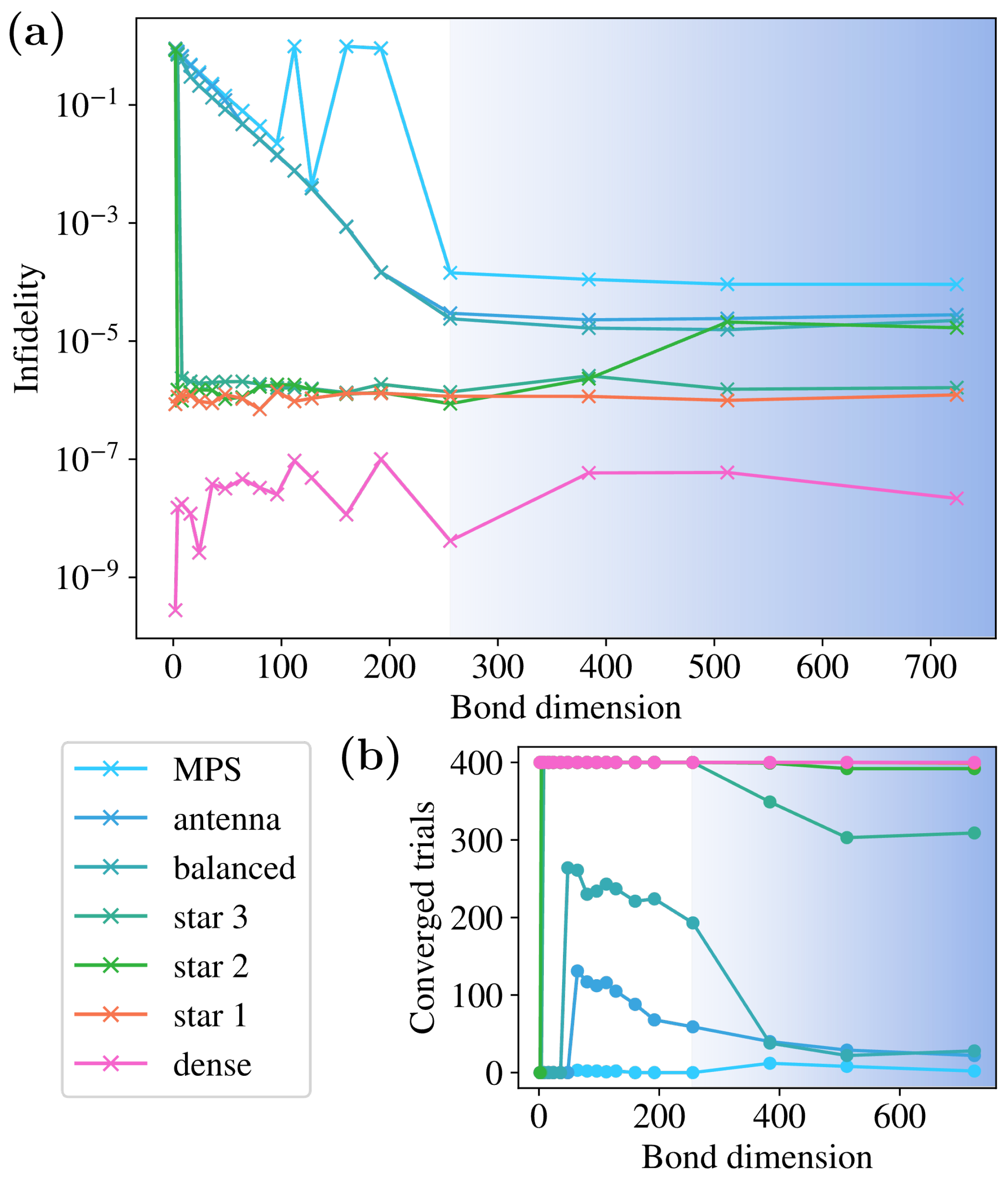
The training described in the previous sections reveals that the connectivity of the tensor network structure directly affects the maximum precision that they can reach. In Figure 4, we show how the infidelities for simulations of a system of sites approach 0, and thus improve, as we increase the bond dimension of the structure. They plateau when the maximal bond dimension is reached, which is to be expected from the point of view of the complexity of the quantum state, but it proves that the redundant information does not help the training procedure. In the inset, we can see how this effect correlates with the maximum distance between nodes in the structure, as highlighted in Figure 1. This means that structures that are more dense, in the sense of proximity between nodes, perform better in the training. This is the case even if the bond dimension is high enough to represent the target state perfectly (), for which ideally, the infidelity should decrease to machine precision for any structure. We also see that increasing the amount of information that the TN can store, which we do by using bond dimensions beyond , does not help the training and, in fact, hurts the success rate, as we see below. For the PEPS, we observe that the first data point with good convergence happens for a large “size of largest tensor”. This is due to the structure of the PEPS, as the largest tensor grows as . Since the bond dimension must be an integer, this number jumps from being small to . For a tensor in a tree structure, each bond dimension is bounded by the number of nodes it connects to, meaning that the largest tensor is bounded by , explaining the vertical alignment of the points.
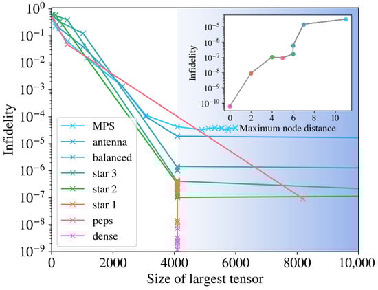
Figure 4.
Training performance measured with infidelity as a function of the largest tensor in the TN, for sites. The size of the tensors was controlled with bond dimension for each of the geometries in Figure 1. Trainings in the blue shaded area use a bond dimension . In the inset, the best infidelity reached against the maximum node distance of the TN structure is given. The ordering and colors follow that of the legend.
In Figure 5, we show a training with larger geometries () and plot the infidelities against bond dimension. The denser structures achieve high fidelity for low bond dimensions, whereas those that are less dense need to reach . Beyond underlining the previous conclusions on infidelity vs. structure density, we can see that even with 400 trials, the MPS training fails to converge, showing its shortcomings in this kind of training and agreeing with current research around barren plateaus (discussed in Section 2.5). The convergence of the training with and shows that this is not due to the structure not being able to store enough information, but to the training process. In Figure 5b, we plot the number of trainings that cross the threshold of , seeing that they decrease with bond dimension. For the most powerful structures (dense, star1, and star2), the decrease is not meaningful. For the rest, the decrease is more pronounced in the regime where , showing that the additional information in the structure makes the training harder, even though, as seen above, this does not translate into improved infidelity.
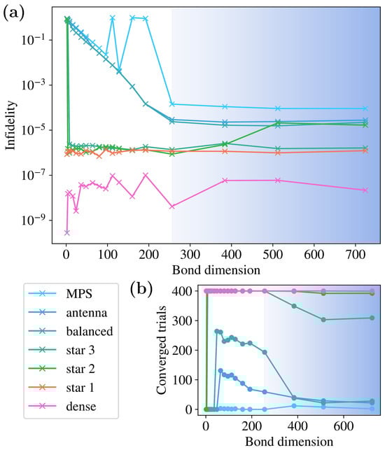
Figure 5.
Training performance measured with infidelity as a function of bond dimension, for sites, in (a). For some bond dimensions in the MPS, none of the trainings reach a good infidelity. The number of trainings that cross a threshold for infidelity is plotted in (b), showing a decrease with the amount of information in the structure, as measured using the bond dimension . The blue shaded area indicates , and colors in both plots follow the same legend.
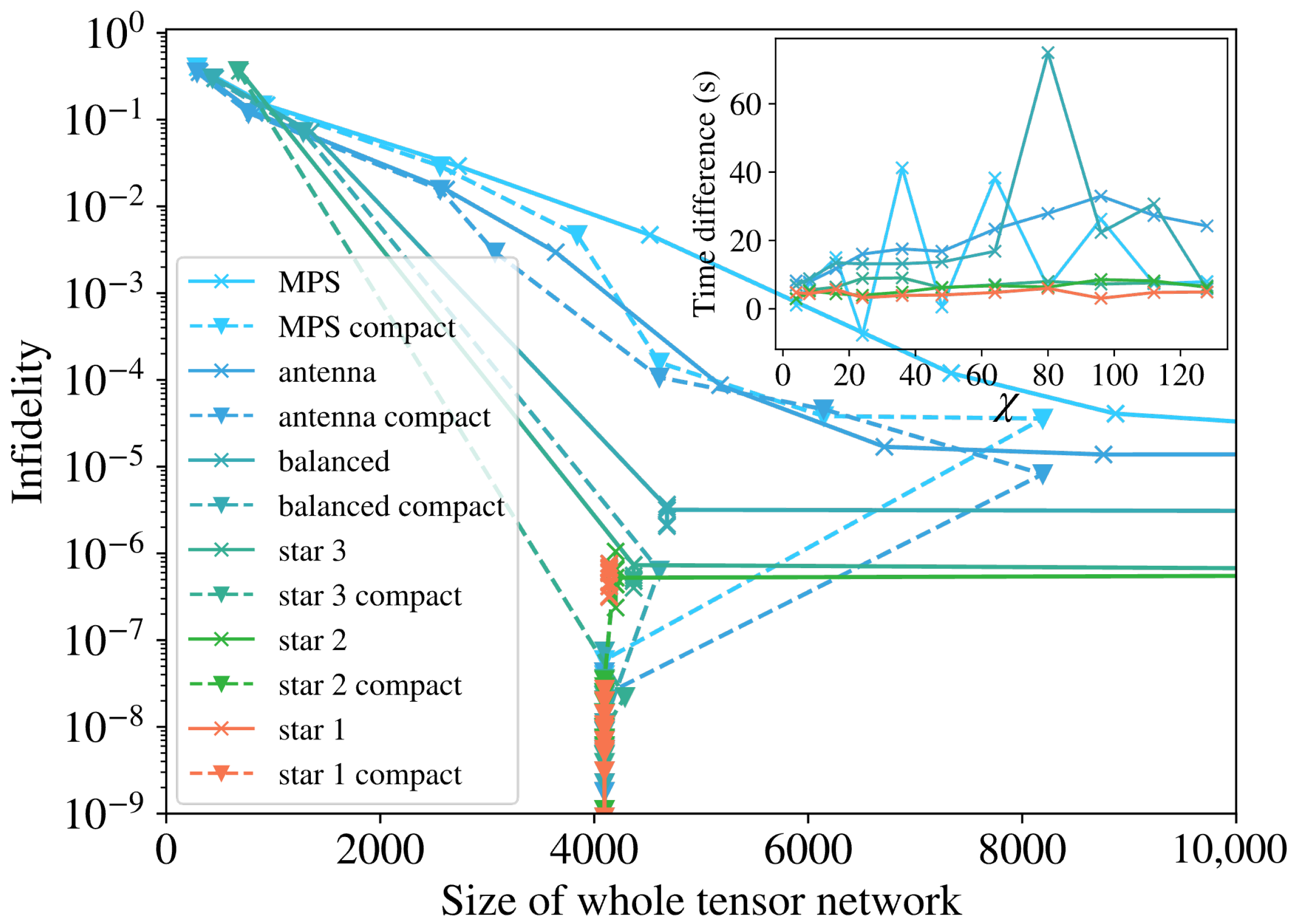
The compactification approach shown in Figure 3 is not shown in the previous plots, as doing so with leads to a single large tensor and there would be no difference between structures. To visualize the effect, we need to test it with reduced bond dimensions, but for random quantum states, this would lead to very high infidelities. We can, however, use the hidden data structure of Figure 2 to prepare targets with reduced complexity equivalent to a limited , and perform the training using that same . In Figure 6, we show the results of such training and see that for each geometry, the corresponding compact version trains better by either achieving the same precision at a smaller bond dimension or reaching lower infidelities at the same bond dimension. This is visible, as the dashed lines (for compact TN) always run closer to the origin, below the solid lines (for regular TN) on the y axis and to the left on the x axis. We see that the last points for each line, corresponding to the biggest , collapse to the area where the dense trainings lie, because the threshold for the compactification is high enough to reduce them to a single tensor.
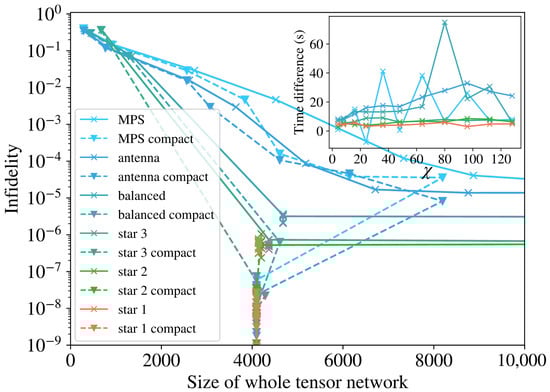
Figure 6.
Training performance measured with infidelity as a function of the full size of the tensor network for the examples in Figure 1, and the compact version of each geometry that follows from Figure 3. The last data points for the compact TNs decrease in size because the compact threshold is high enough to contract them into a single tensor.
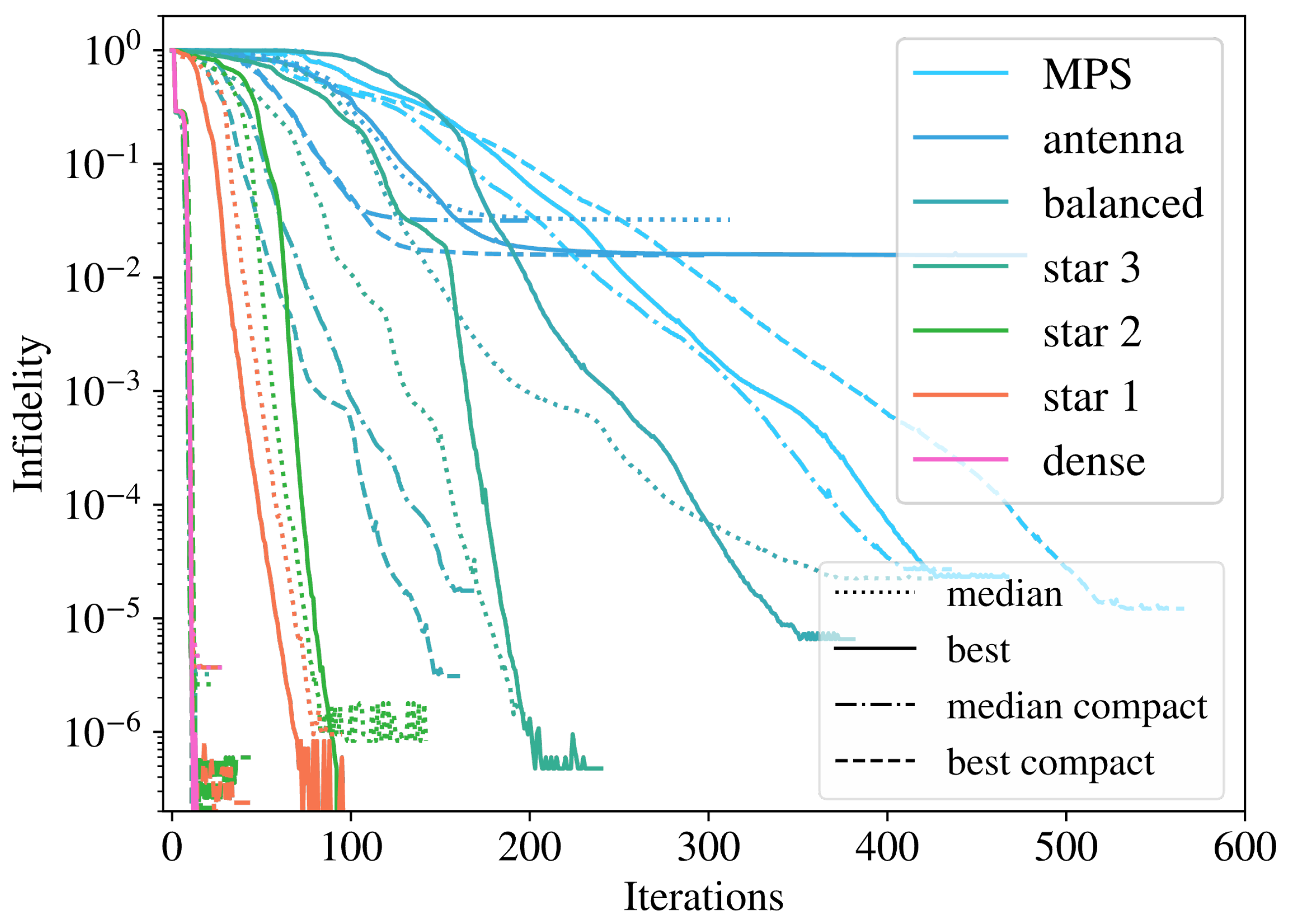
An example of the training evolution across iterations is shown in Figure 7, for , highlighting differences in the behavior of all the studied geometries. Across a run of 100 trainings, we include both the best training and the median training, ordered according to the final infidelity reached, as the difference in orders of magnitude skews the arithmetic mean. The results indicate that the compact versions of geometries train faster and better than their regular counterparts, not only in the best case scenario but also on average. This improvement is consistent with our findings of smaller infidelity with growing density, as compactification reduces the maximal node distance and other similarly related measures of graph connectivity that correlate with it. We also see that below infidelities of , there are some numerical stabilities that impact the denser structures and were the cause for the high variance in the dense training of Figure 5.
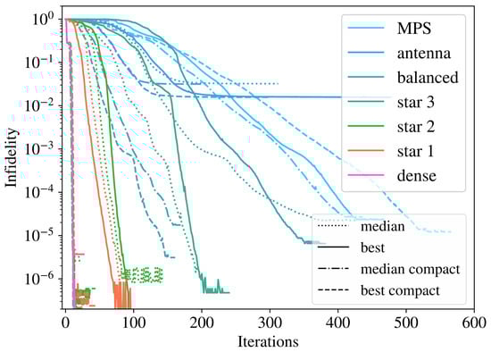
Figure 7.
Example of training with sites for each geometry and using low bond dimension to compare them with the compact tensor network structures. Solid (dashed) lines represent the best regular (compact) training, and dotted (dot-dashed) represent the regular (compact) median training, ordered according to final infidelity.
Lastly, we compare the impact of accelerated simulation on the time and energy efficiency of the training. The results in Figure 8 compare a training using 20 CPU cores against one using the same number of cores in addition to 1 GPU, with single and double precision in the GPU case. We can see an advantage in the GPU acceleration for the largest size when comparing trainings with the same precision (double). The default precision (single) when using a GPU with Jax introduced some error in the results, leading to infidelities between 1 and 2 orders of magnitude larger than the main findings above. This could be good enough in some settings, and can be leveraged to achieve performance enhancements at smaller sizes, starting at . In terms of energy, we see that GPU-accelerated trainings draw around more power, which means that the total energy cost (power · time) is smaller when the training time is smaller by , as is the case for . Additionally, we identified that only part of the optimization was able to effectively use the GPU, reducing the impact of the advantage and contributing to the time advantage becoming apparent only for the largest sizes.
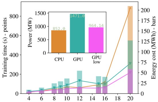
Figure 8.
The time cost (left axis, points) and energy cost (right axis, bars) of the training in this work for different sizes of the system, adding together all reviewed geometries. We use 20 CPU cores and 20 CPU cores + GPU, both with high and reduced precision, labeled as “CPU”, “GPU”, and “GPU low”, respectively. In the inset, the average power needed for each training is presented.
5. Conclusions and Outlook
The experiments and training pipeline presented in this work contribute to current research on TN architectures, starting with a surrogate tensor contraction that enables further research in heterogeneous geometries. Our main findings relate to how different structures reach increasing levels of quality when training them to learn random states. Specifically, more dense geometries reach smaller errors faster both in terms of time and iterations, despite an increased contraction cost. Our interpretation is that the way the TN structure connects and distributes the information that it stores is much more important than the total amount of information it can store. Evidence for this includes the worse performance of the MPS and some tree TNs with maximal bond dimensions, despite being as complex as their denser counterparts, as well as the lack of improvement when allowing artificially large bond dimensions.
The emergence of barren plateaus is relevant in any gradient-based training, and it is expected to appear when using a global loss function based on infidelity, as happens in our experiment. It has previously been linked to MPSs, with tree TNs and other more complex structures being less prone to exhibiting them. We have expanded on these findings by showing that their behavior is tied to the density of the structure, with barren plateaus being absent for very dense structures and becoming slightly more prominent as sparsity increases. For the MPS, specifically, the training even fails to converge for sites unless using hundreds of trials, but performs well for denser structures.
Memory limits in the training of tensor networks are dependent on the largest tensor contraction at any point as they rely on the transfer of large tensors from fast to slow memory. Regardless, decreasing the total memory required contributes to reducing the overall duration of the computation by minimizing the movements of large tensors between memories. We have also introduced a compactification of tree TN structures, using our training examples to prove that it not only reduces the total memory needed but also improves the quality and speed of the training. The latter is due to a reduced number of iterations, as the cost of the contractions themselves increases slightly with the compactification. These results are consistent with the density effect observed.
Finally, we have showcased an application of existing tensor network libraries with HPC resources, and also characterized performance improvements with the use of accelerated hardware in this same setting, which is very impactful for the large-scale setting that these types of experiments are usually executed on. Due to the nature of the simulations, these benchmarks are also relevant for similar machine learning techniques in HPC.
Overall, this work contributes to better understanding the training of TNs, and will also have an impact on dynamical approaches to finding optimal structures. We think it is of great interest to extend the study of these geometries beyond gradient training towards powerful methods like DMRG or TEBD in the future. Similarly, with the proposed surrogate procedure, one can test if entanglement structures hidden in a single tensor can be learned with specific TN ansatzes, either using gradient methods or DMRG.
Author Contributions
Conceptualization, S.M.-L. and A.G.-S.; methodology, S.M.-L.; software, S.M.-L.; validation, S.M.-L. and A.G.-S.; formal analysis, S.M.-L.; investigation, S.M.-L.; resources, S.M.-L. and A.G.-S.; data curation, S.M.-L.; writing—original draft preparation, S.M.-L.; writing—review and editing, S.M.-L. and A.G.-S.; visualization, S.M.-L.; supervision, A.G.-S.; project administration, S.M.-L. and A.G.-S.; funding acquisition, A.G.-S. All authors have read and agreed to the published version of the manuscript.
Funding
The authors acknowledge financial support from EU grant HORIZON-EIC-2022-PATHFINDEROPEN-01-101099697, QUADRATURE, and from Generalitat de Catalunya grant 2021SGR00907, and funding from the Spanish Ministry for Digital Transformation and Civil Service of the Spanish Government through the QUANTUM ENIA project call Quantum Spain, EU, through the Recovery, Transformation and Resilience Plan—NextGenerationEU within the framework of Digital Spain 2026.
Data Availability Statement
All the data from our figures was produced with the code and scripts publicly available at https://github.com/bsc-quantic/strucTN (accessed on 19 January 2025).
Acknowledgments
We want to thank Sergio Sánchez and Germán Navarro for engaging in fruitful discussions around tensor networks and HPC performance, Berta Casas for her eye for plots, and the rest of the BSC team for their support and comments.
Conflicts of Interest
Author Artur Garcia-Saez was employed by the company Qilimanjaro Quantum Tech. The remaining authors declare that the research was conducted in the absence of any commercial or financial relationships that could be construed as a potential conflict of interest. The funders had no role in the design of the study; in the collection, analyses, or interpretation of data; in the writing of the manuscript; or in the decision to publish the results.
References
- Cirac, J.I.; Perez-Garcia, D.; Schuch, N.; Verstraete, F. Matrix Product States and Projected Entangled Pair States: Concepts, Symmetries, and Theorems. Rev. Mod. Phys. 2021, 93, 045003. [Google Scholar] [CrossRef]
- Markov, I.L.; Shi, Y. Simulating Quantum Computation by Contracting Tensor Networks. SIAM J. Comput. 2008, 38, 963–981. [Google Scholar] [CrossRef]
- Gray, J.; Chan, G.K.L. Hyperoptimized Approximate Contraction of Tensor Networks with Arbitrary Geometry. Phys. Rev. X 2024, 14, 011009. [Google Scholar] [CrossRef]
- Vidal, G. Efficient Classical Simulation of Slightly Entangled Quantum Computations. Phys. Rev. Lett. 2003, 91, 147902. [Google Scholar] [CrossRef] [PubMed]
- McCulloch, I.P. Infinite Size Density Matrix Renormalization Group, Revisited. arXiv 2008, arXiv:0804.2509. [Google Scholar]
- Vidal, G. Entanglement Renormalization. Phys. Rev. Lett. 2007, 99, 220405. [Google Scholar] [CrossRef] [PubMed]
- Verstraete, F.; Cirac, J.I. Renormalization algorithms for Quantum-Many Body Systems in two and higher dimensions. arXiv 2004, arXiv:cond-mat/0407066. [Google Scholar]
- Georgescu, I.; Ashhab, S.; Nori, F. Quantum simulation. Rev. Mod. Phys. 2014, 86, 153–185. [Google Scholar] [CrossRef]
- Begušić, T.; Gray, J.; Chan, G.K.L. Fast and converged classical simulations of evidence for the utility of quantum computing before fault tolerance. Sci. Adv. 2024, 10, eadk4321. [Google Scholar] [CrossRef]
- Kim, Y.; Eddins, A.; Anand, S.; Wei, K.X.; van den Berg, E.; Rosenblatt, S.; Nayfeh, H.; Wu, Y.; Zaletel, M.; Temme, K.; et al. Evidence for the utility of quantum computing before fault tolerance. Nature 2023, 618, 500–505. [Google Scholar] [CrossRef] [PubMed]
- Verstraete, F.; Murg, V.; Cirac, J. Matrix product states, projected entangled pair states, and variational renormalization group methods for quantum spin systems. Adv. Phys. 2008, 57, 143–224. [Google Scholar] [CrossRef]
- Schollwöck, U. The density-matrix renormalization group in the age of matrix product states. Ann. Phys. 2011, 326, 96–192. [Google Scholar] [CrossRef]
- Stoudenmire, E.M.; Schwab, D.J. Supervised Learning with Quantum-Inspired Tensor Networks. arXiv 2017, arXiv:1605.05775. [Google Scholar]
- Wang, J.; Roberts, C.; Vidal, G.; Leichenauer, S. Anomaly Detection with Tensor Networks. arXiv 2020, arXiv:2006.02516. [Google Scholar]
- Orús, R. Tensor networks for complex quantum systems. Nat. Rev. Phys. 2019, 1, 538–550. [Google Scholar] [CrossRef]
- Christandl, M.; Lysikov, V.; Steffan, V.; Werner, A.H.; Witteveen, F. The resource theory of tensor networks. Quantum 2024, 8, 1560. [Google Scholar] [CrossRef]
- Ye, K.; Lim, L.H. Tensor network ranks. arXiv 2019, arXiv:1801.02662. [Google Scholar]
- Zeng, J.; Li, C.; Sun, Z.; Zhao, Q.; Zhou, G. tnGPS: Discovering Unknown Tensor Network Structure Search Algorithms via Large Language Models (LLMs). arXiv 2024, arXiv:2402.02456. [Google Scholar]
- Li, C.; Sun, Z. Evolutionary Topology Search for Tensor Network Decomposition. In Proceedings of the 37th International Conference on Machine Learning, PMLR 2020, Virtual Event, 13–18 July 2020; Daumé, H., III, Singh, A., Eds.; Proceedings of Machine Learning Research. Volume 119, pp. 5947–5957. [Google Scholar]
- Hikihara, T.; Ueda, H.; Okunishi, K.; Harada, K.; Nishino, T. Automatic structural optimization of tree tensor networks. Phys. Rev. Res. 2023, 5, 013031. [Google Scholar] [CrossRef]
- Evenbly, G. A Practical Guide to the Numerical Implementation of Tensor Networks I: Contractions, Decompositions and Gauge Freedom. arXiv 2022, arXiv:2202.02138. [Google Scholar] [CrossRef]
- Zhao, Y.Q.; Li, R.G.; Jiang, J.Z.; Li, C.; Li, H.Z.; Wang, E.D.; Gong, W.F.; Zhang, X.; Wei, Z.Q. Simulation of quantum computing on classical supercomputers with tensor-network edge cutting. Phys. Rev. A 2021, 104, 032603. [Google Scholar] [CrossRef]
- Cervero Martín, E.; Plekhanov, K.; Lubasch, M. Barren plateaus in quantum tensor network optimization. Quantum 2023, 7, 974. [Google Scholar] [CrossRef]
- Liu, Z.; Yu, L.W.; Duan, L.M.; Deng, D.L. Presence and Absence of Barren Plateaus in Tensor-Network Based Machine Learning. Phys. Rev. Lett. 2022, 129, 270501. [Google Scholar] [CrossRef] [PubMed]
- Menczer, A.; van Damme, M.; Rask, A.; Huntington, L.; Hammond, J.; Xantheas, S.S.; Ganahl, M.; Legeza, Ö. Parallel implementation of the Density Matrix Renormalization Group method achieving a quarter petaFLOPS performance on a single DGX-H100 GPU node. arXiv 2024, arXiv:2407.07411. [Google Scholar] [CrossRef] [PubMed]
- Benenti, G.; Casati, G.; Davide Rossini, G. Entanglement and non-classical correlations. In Principles of Quantum Computation and Information; World Scientifics: Singapore, 2018; Chapter 6; pp. 241–286. [Google Scholar] [CrossRef]
- Horodecki, R.; Horodecki, P.; Horodecki, M.; Horodecki, K. Quantum entanglement. Rev. Mod. Phys. 2009, 81, 865–942. [Google Scholar] [CrossRef]
- Horodecki, P.; Rudnicki, Ł.; Życzkowski, K. Multipartite entanglement. arXiv 2024, arXiv:2409.04566. [Google Scholar]
- Nielsen, M.A.; Chuang, I.L. Introduction to Quantum Mechanics. In Quantum Computation and Quantum Information: 10th Anniversary Edition; Cambridge University Press: Cambridge, UK, 2010; pp. 60–119. [Google Scholar]
- Orus, R. A Practical Introduction to Tensor Networks: Matrix Product States and Projected Entangled Pair States. Ann. Phys. 2014, 349, 117–158. [Google Scholar] [CrossRef]
- Sharma, M.; Markopoulos, P.P.; Saber, E.; Asif, M.S.; Prater-Bennette, A. Convolutional Auto-Encoder with Tensor-Train Factorization. In Proceedings of the 2021 IEEE/CVF International Conference on Computer Vision Workshops (ICCVW), Montreal, BC, Canada, 11–17 October 2021; pp. 198–206. [Google Scholar] [CrossRef]
- Su, Z.; Zhou, Y.; Mo, F.; Simonsen, J.G. Language Modeling Using Tensor Trains. arXiv 2024, arXiv:2405.04590. [Google Scholar]
- Oseledets, I.V. Tensor-Train Decomposition. SIAM J. Sci. Comput. 2011, 33, 2295–2317. [Google Scholar] [CrossRef]
- Affleck, I.; Kennedy, T.; Lieb, E.H.; Tasaki, H. Rigorous Results on Valence-Bond Ground States in Antiferromagnets. Phys. Rev. Lett. 1987, 59, 799–802. [Google Scholar] [CrossRef]
- Evenbly, G.; Vidal, G. Tensor Network States and Geometry. J. Stat. Phys. 2011, 145, 891–918. [Google Scholar] [CrossRef]
- Eisert, J.; Cramer, M.; Plenio, M.B. Area Laws for the Entanglement Entropy—A Review. Rev. Mod. Phys. 2010, 82, 277–306. [Google Scholar] [CrossRef]
- Shi, Y.Y.; Duan, L.M.; Vidal, G. Classical simulation of quantum many-body systems with a tree tensor network. Phys. Rev. A 2006, 74, 022320. [Google Scholar] [CrossRef]
- Okunishi, K.; Ueda, H.; Nishino, T. Entanglement bipartitioning and tree tensor networks. Prog. Theor. Exp. Phys. 2023, 2023, 023A02. [Google Scholar] [CrossRef]
- Haghshenas, R.; O’Rourke, M.J.; Chan, G.K.L. Conversion of projected entangled pair states into a canonical form. Phys. Rev. B 2019, 100, 054404. [Google Scholar] [CrossRef]
- Hyatt, K.; Stoudenmire, E.M. DMRG Approach to Optimizing Two-Dimensional Tensor Networks. arXiv 2020, arXiv:1908.08833. [Google Scholar]
- Hikihara, T.; Ueda, H.; Okunishi, K.; Harada, K.; Nishino, T. Visualization of Entanglement Geometry by Structural Optimization of Tree Tensor Network. arXiv 2024, arXiv:2401.16000. [Google Scholar]
- Lu, J.; Gong, P.; Ye, J.; Zhang, J.; Zhang, C. A Survey on Machine Learning from Few Samples. arXiv 2023, arXiv:2009.02653. [Google Scholar] [CrossRef]
- Fuksa, J.; Götte, M.; Roth, I.; Eisert, J. A quantum inspired approach to learning dynamical laws from data—block-sparsity and gauge-mediated weight sharing. Mach. Learn. Sci. Technol. 2024, 5, 025064. [Google Scholar] [CrossRef]
- Cerezo, M.; Verdon, G.; Huang, H.Y.; Cincio, L.; Coles, P.J. Challenges and opportunities in quantum machine learning. Nat. Comput. Sci. 2022, 2, 567–576. [Google Scholar] [CrossRef] [PubMed]
- Wu, X.C.; Di, S.; Cappello, F.; Finkel, H.; Alexeev, Y.; Chong, F.T. Memory-Efficient Quantum Circuit Simulation by Using Lossy Data Compression. arXiv 2018, arXiv:1811.05630. [Google Scholar]
- Pan, F.; Gu, H.; Kuang, L.; Liu, B.; Zhang, P. Efficient Quantum Circuit Simulation by Tensor Network Methods on Modern GPUs. arXiv 2024, arXiv:2310.03978. [Google Scholar] [CrossRef]
- Sanchez-Ramirez, S.; Conejero, J.; Lordan, F.; Queralt, A.; Cortes, T.; Badia, R.M.; Garcia-Saez, A. RosneT: A Block Tensor Algebra Library for Out-of-Core Quantum Computing Simulation. In Proceedings of the 2021 IEEE/ACM Second International Workshop on Quantum Computing Software (QCS), St. Louis, MO, USA, 15 November 2021; IEEE: Piscataway, NJ, USA, 2021; pp. 1–8. [Google Scholar] [CrossRef]
- Vidal, G. Efficient Simulation of One-Dimensional Quantum Many-Body Systems. Phys. Rev. Lett. 2004, 93, 040502. [Google Scholar] [CrossRef] [PubMed]
- Hashizume, T.; Halimeh, J.C.; McCulloch, I.P. Hybrid infinite time-evolving block decimation algorithm for long-range multidimensional quantum many-body systems. Phys. Rev. B 2020, 102, 035115. [Google Scholar] [CrossRef]
- McClean, J.R.; Boixo, S.; Smelyanskiy, V.N.; Babbush, R.; Neven, H. Barren plateaus in quantum neural network training landscapes. Nat. Commun. 2018, 9, 4812. [Google Scholar] [CrossRef] [PubMed]
- Cerezo, M.; Larocca, M.; García-Martín, D.; Diaz, N.L.; Braccia, P.; Fontana, E.; Rudolph, M.S.; Bermejo, P.; Ijaz, A.; Thanasilp, S.; et al. Does provable absence of barren plateaus imply classical simulability? Or, why we need to rethink variational quantum computing. arXiv 2024, arXiv:2312.09121. [Google Scholar]
- Schuld, M.; Killoran, N. Is Quantum Advantage the Right Goal for Quantum Machine Learning? PRX Quantum 2022, 3, 030101. [Google Scholar] [CrossRef]
- Basheer, A.; Feng, Y.; Ferrie, C.; Li, S.; Pashayan, H. On the Trainability and Classical Simulability of Learning Matrix Product States Variationally. arXiv 2024, arXiv:2409.10055. [Google Scholar]
- Miao, Qiang and Barthel, Thomas Isometric tensor network optimization for extensive Hamiltonians is free of barren plateaus. Phys. Rev. A 2024, 109, L050402. [CrossRef]
- Liu, D.C.; Nocedal, J. On the limited memory BFGS method for large scale optimization. Math. Program. 1989, 45, 503–528. [Google Scholar] [CrossRef]
- Baydin, A.G.; Pearlmutter, B.A.; Radul, A.A.; Siskind, J.M. Automatic differentiation in machine learning: A survey. arXiv 2018, arXiv:1502.05767. [Google Scholar]
- Gray, J. quimb: A python package for quantum information and many-body calculations. J. Open Source Softw. 2018, 3, 819. [Google Scholar] [CrossRef]
- Bradbury, J.; Frostig, R.; Hawkins, P.; Johnson, M.J.; Leary, C.; Maclaurin, D.; Necula, G.; Paszke, A.; VanderPlas, J.; Wanderman-Milne, S.; et al. JAX: Composable Transformations of Python+NumPy Programs, Software Version 0.3.13; GitHub, Inc.: San Francisco, CA, USA, 2018; Available online: http://github.com/jax-ml/jax (accessed on 19 January 2025).
- MareNostrum 5. Available online: https://www.bsc.es/marenostrum/marenostrum-5 (accessed on 19 January 2025).


Disclaimer/Publisher’s Note: The statements, opinions and data contained in all publications are solely those of the individual author(s) and contributor(s) and not of MDPI and/or the editor(s). MDPI and/or the editor(s) disclaim responsibility for any injury to people or property resulting from any ideas, methods, instructions or products referred to in the content. |
© 2025 by the authors. Licensee MDPI, Basel, Switzerland. This article is an open access article distributed under the terms and conditions of the Creative Commons Attribution (CC BY) license (https://creativecommons.org/licenses/by/4.0/).