Comparison of Fixed- and Mixed-Effects Approaches to Taper Modeling for Scots Pine in West Poland

Abstract

Diameter measurements along the stem, which are the basis for taper models, usually have a hierarchical structure. Mixed-effects models, where fixed and random effects are distinguished, are a possible solution for this type of data. However, in order to fully absorb the potential of this method, random effects prediction, which requires additional measurements (diameter along stem), is recommended. This article presents a comparison of various fitting methods (mixed- and fixed-effects model approaches) of the variable-exponent taper model created by Kozak for determining the outside bark diameter along the stem and predicting the tree volume of Scots pine trees in west Poland. During the analysis, it was assumed that no additional measured data were available for practical use; therefore, for the mixed-effects model approach, fixed effects prediction without random effects was applied. Both fitting strategies were compared based on modeling and an independent validation data set. The comparison of mixed- and fixed-effects fitting strategies for the diameter along the stem indicated that the taper model fitted using the mixed-effects model approach better fit the data. Moreover, the error rate for the total tree volume prediction for the independent data set was lower for the mixed-effects model solution than for the fixed-effects one.

1. Introduction

The tree stem shape, which, in many cases, is characterized by analyzing the variability of tree parameters (mainly diameter) relative to the height change along the tree [1], as well as the volume resulting from it, is one of the most important types of theoretical and practical information used in the forestry and timber industry. One of the ways to define the longitudinal shapes of trees is to develop special models known as taper functions. These models allow us to determine the diameter of a tree at any height, and as a consequence, the desired volume and biomass [2], as well as the amounts of various products that can be obtained from a tree after cutting [3].

One group of taper models are linear models that describe the longitudinal shape of a tree using a certain number of diameters at different relative tree heights [4,5]. The linear model, developed on the basis of 15 relative tree heights, determines the longitudinal shape of the tree on the basis of the share of 15 sections of the tree volume was the first Polish taper model elaborated for Scots pine [6]. Notwithstanding, nonlinear models represent the largest group of solutions found in the literature. In the simplest nonlinear cases, the shape of the stem can be mapped using a single mathematical function [7]. This may be a polynomial [8], power [9], or exponential function [10]. It is also possible to use a variable shape equation [11], assuming that the longitudinal shape varies along the tree [12,13,14]. Nonlinear taper models composed of two or more segments created using various mathematical functions are also available [15,16], as the shapes of various tree stem segments can be approximated with different geometric solids [17].

Forest inventory data, including diameter measurements along the stem used as a basis for taper models, are often characterized by a hierarchical structure, which contains information about individual diameters, trees, or plots. The mixed-effects models, where the fixed and random effects are distinguished, are possible solutions for these types of data [18]. The fixed part of these models allows data for a typical basic group (e.g., tree or plot) to be modeled, whereas the random part describes the difference between each group and the typical one, thus enabling descriptions of the specific relationships among all groups of the dataset [19]. Random effects can be applied for modeling within repeated measurements along the stem and between-tree correlations [20]. In addition, during random effects prediction, it is possible to include different levels of data grouping [11,21,22]. In this context, the Bayesian estimator or best linear unbiased predictor (BLUP) are possible solutions for the prediction of random effects in taper models [20,23]. Considering the possibilities of using mixed-effects models, it is possible to select various strategies. One possibility is to define random-effects on individual tree level (without autocorrelation modeling). This approach allows us to explain as large a proportion of the between-tree variation as possible [24]. Other elements worth considering are the practical use of the created model [11] and the ability to analyze large data sets [25]. In addition, convergence problems during model fitting should also be considered [26,27]. Notwithstanding, in practical applications of the taper model, where additional measurements of the tree diameter along the stem are necessary for random effects prediction, fixed effects prediction can be applied [26].

Scots pine is the main forest-forming species in Poland. It covers 5367 thousand hectares, which translates into a 58.2% share of this tree species in Polish forests. It mainly occupies dry, oligotrophic habitats (dry, fresh, and mixed fresh coniferous forest site types according to Polish site classification [28]). The average age of Scots pine stands in Poland is 60 years. Growing stock equals 1598 million cubic meters (61.2%), while the average gross timber volume per hectare is 298 cubic meters, and the 10-year timber removal rate for this tree species equals 17.76 cubic meters per hectare [29].

Currently, in Poland, in order to determine the tree volume or merchantable volume of an analyzed tree species, one option is to apply empirical equations [30,31,32]. Another possible solution is to use an indirect taper model; however, this utilizes a function involving the determination of the volume share of 15 stem sections [33,34,35]. No taper model allows us to directly reach information about the longitudinal shape of the tree based on easily measurable tree features such as the height and diameter at breast height. Taking into account the above issues, the objectives of this study were to (i) to fill the gap in the existing models by providing the first direct and nonlinear Polish taper model for Scots pine using data from typical oligotrophic sites in west Poland, (ii) to fit the example of a taper model (namely, Kozak 1997) to the diameter along the stem of pine trees as a fixed-effects model and mixed-effects model, (iii) to compare both fitting strategies for measuring the diameter along the stem, and (iv) to compare both strategies for determining the tree volume, taking into account similar modeling data sets, as well as independent (validation) data, and considering the available Polish empirical volume equation [31].

2. Materials and Methods

The data used for modeling consisted of information and measurements collected from 18 Scots pine stands located in west Poland (Lubsko and Gubin forest districts, Regional Directorate of State Forests in Zielona Góra, Figure 1). Sample plots were located on oligotrophic sites typical for pine trees (i.e., dry, fresh, and fresh mixed coniferous forest, according to the Polish forest site classification). Borders of the chosen rectangular sample plots were permanently marked in the field. The size of each plot was set in such a way that each plot comprised at least 200 trees. The diameter at breast height (DBH) of all live trees (accuracy 0.01 cm) was measured on all plots, as well as at 25 heights (H) (accuracy 0.01 m) to build a local height–diameter model. From each stand, five model trees representing the entire diameter range were chosen proportionally to diameter classes and felled (90 trees in total). The heights of the analyzed trees varied from 6.95 to 25.65 m, and the DBH varied from 6.7 to 31.5 cm. The mean values of these parameters were 15.51 m and 15.7 cm, respectively (

Table 1. Characteristics of the model trees for both data sets: diameter at breast height (DBH, cm), tree height (H, m), tree volume (V, m³).

Statistics	Modeling Data			Independent Data
	DBH	H	V	DBH	H	V
Minimum	6.7	6.95	0.0153	6.85	9.18	0.0214
Median	14.9	15.03	0.1272	21.23	22.37	0.3199
Mean	15.7	15.51	0.1923	20.87	19.84	0.3984
Maximum	31.5	25.65	0.8642	34.25	26.95	1.0229
Stand. Dev.	6.04	3.93	0.1808	7.94	5.83	0.307
Stand. Error	0.64	0.41	0.0191	1.62	1.19	0.0627

).

Each model tree was measured section-wise (1 m section length, measurements at 0.5 m, 1.5 m, 2.5 m, etc.) to determine its diameter outside the bark (Figure 2). The volumes of these trees were calculated using the sectional Huber’s equation.

Apart from the plots used for building taper equations, independent data were used to validate the created models. The validation dataset was collected from eight Scots pine stands in the western part of Poland (Sława Śląska and Sulechów forest districts, Regional Directorate of State Forests in Zielona Góra, Figure 1). Sample plots of varying size (comprising at least 100 live standing pine trees) were established on the most prevalent site conditions for pine. The DBH of all trees was measured on all plots, as well as 25 tree heights, and height–diameter curves were created, as in the case of the main dataset. At each plot, three model trees representing the whole range of diameter structures were chosen and felled. In total, 24 model trees were used for further analyses (Table 1). The height of the analyzed trees varied from 9.18 to 26.95 m, and the DBH varied from 6.85 to 34.25 cm. The average values of these parameters were 19.84 m and 20.87 cm, respectively (Table 1). Felled trees were measured section-wise (1 m section length, measurements at 0 m, 1 m, 2 m, etc.) to determine their diameters outside the bark. The volumes of these trees were calculated using the sectional Smalian’s equation.

Despite the fact that modeling and validation volume data were obtained using different equations (sectional Huber’s and Smalian’s one), the resulting volumes are very close to the true ones, being practically accurate. A short length of sections, the top and bottom diameter ratio close to 1 for each section, and errors of various sections having different signs (as they actually cancel out), cause the resulting differences in the total tree volume obtained using different equations to differ from the true values by a maximum of ±1%. Such research dealing with empirical accuracy of sectional equations (applied to real trees, stems or bolts, not theoretical, applied to solids of revolutions, such as paraboloid, neiloid or cone) are rather scarce [36], but available, mostly in classical textbooks on forest mensuration [12,37,38,39]. This is because of difficulties in the determination of the true (real) volume of trees, which requires using fluid (water) displacement methods (xylometry) to get reference values.

2.1. Taper Function

Considering the practical application of the created model, we chose a solution that used DBH and H to define the longitudinal tree shape, which, as a consequence, translated into the possibility of determining its volume. We applied a solution based on a previously tested function [26], the 8-parameter taper model developed by Kozak [7]:

$$\begin{gathered} D=b_{1}DB{H}^{b_2}{H}^{b_3}{\left[\frac{1-\sqrt{q}}{1-\sqrt{t}}\right]}^{b_4{\left(\frac{1-\sqrt{q}}{1-\sqrt{t}}\right)}^{0.1}}+b_5{q}^4+b_{6}arcsin\left(1-\sqrt{q}\right)+b_7\left(\frac{1}{e^{\frac{DBH}{H}}}\right) \\ +b_{8}DB{H}^{\left(\frac{1-\sqrt{q}}{1-\sqrt{t}}\right)} \end{gathered}$$

(1)

where D as dependent variable is the diameter along the stem (cm), DBH is the diameter at breast height (cm), H is the tree height (m), q is the ratio between the diameter along the stem position and the tree height (h/H), t is the relative breast height (1.30/H), DBH, H, q, t are independent variables, and b_1,…, b₈ are the estimated model parameters.

This model (Equation (1)) was fitted by a fixed-effects (nonlinear least-squares method) and mixed-effects modeling approach. Considering the impacts of individual model parameters on different parts of the modeled tree shape, in the case of mixed-effects model solution, we defined three random parameters (β₁, β₂, β₃). On one hand, the definition of parameters in this way, in connection with adopting the tree as a grouping level, allowed us to avoid highly correlated random effects and convergence problems while, on the other hand, allowed us to consider the between-tree variation in the lower, top, and middle parts of the stem [26]. As a consequence, we obtained the following model:

$$\begin{gathered} D_{ki}=b_{1}DB{H}_k^{b_2}{H}_k^{b_3+{\beta }_{1_k}}{\left[\frac{1-\sqrt{q_{ki}}}{1-\sqrt{t_{ki}}}\right]}^{b_4{\left(\frac{1-\sqrt{q_{ki}}}{1-\sqrt{t_{ki}}}\right)}^{0.1}}+(b_5+{\beta }_{2_k})q_{ki}^4+(b_6+{\beta }_{3_k})arcsin\left(1-\sqrt{q_{ki}}\right)+b_7\left(\frac{1}{e^{\frac{DB{H}_k}{H_k}}}\right) \\ +b_{8}DB{H}_k^{\left(\frac{1-\sqrt{q_{ki}}}{1-\sqrt{t_{ki}}}\right)}+e_{ki} \end{gathered}$$

(2)

where k refers to individual trees.

Models fitted using both strategies were compared based on goodness-of-fit measures such as the coefficient of determination (R²):

$$R^2=1-\frac{{\displaystyle \sum }{\left(y-\widehat{y}\right)}^2}{{\displaystyle \sum }{\left(y-\overline{y}\right)}^2}$$

(3)

where $y$ is a measured diameter along the stem, $\widehat{y}$ is a modeled diameter along the stem, and $\overline{y}$ is a mean value of measured diameter along the stem, root-mean-square error (RMSE):

$$RMSE=\sqrt{\frac{{\displaystyle \sum }{\left(y-\widehat{y}\right)}^2}{n-p}}$$

(4)

where $n$ is the number of diameters along the stem, and $p$ is the number of models’ parameters, and mean error (ME):

$$ME=\frac{{\displaystyle \sum }\left(y-\widehat{y}\right)}{n}$$

(5)

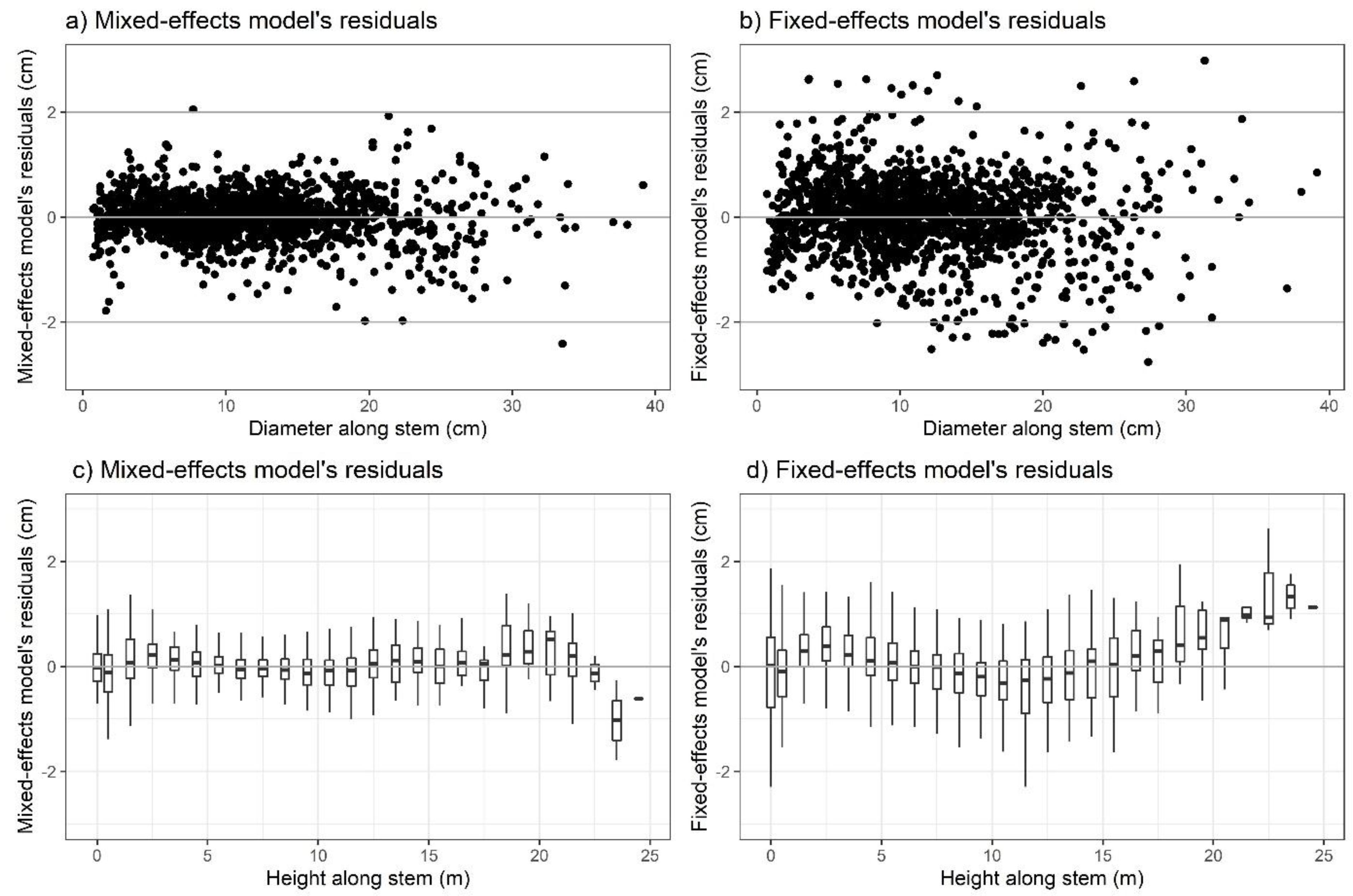
In addition, we evaluated the obtained residuals graphically based on their relationships with the diameter along the stem and the height along the stem. Furthermore, the obtained taper models were graphically compared according to the relative height (tree height/diameter position along stem) and relative diameter (diameter along stem/diameter at the breast height) of the stem.

2.2. Volume Prediction

The volumes of model trees were calculated based on the 1 m section-wise Huber’s equation (modeling data):

$$RV=l_s·\left(g_{s_1}+g_{s_2}+\dots +g_{s_{n-1}}+g_{s_n}\right)+V_a$$

(6)

where $RV$ is the reference volume (m³), $l_s$ is the length of the section (m), $g_{s_1}$, $g_{s_2}$, $g_{s_{n-1}}$, $g_{s_n}$ is a basal area in the middle of the individual sections (m²), and $V_a$ is the volume of last section (m³), and Smalian’s equation (validation data):

$$RV=l_s·\left(\frac{g_0+g_n}{2}+g_1+g_2+g_3+\dots +g_{n-1}\right)+V_a$$

(7)

where $g_0$, $g_n$, $g_1$, $g_2$, $g_3$, $g_{n-1}$ is a basal area at the beginning and end of individual sections (m²).

During volume calculations based on the taper models obtained using both strategies, we adopted the assumption that additional measurements of tree diameter along the stem, which are necessary for random effects prediction, were not available. In the case of the fixed-effects model (first strategy), we used all fitted model parameters, whereas for the mixed-effects model, we applied fixed parameters only. For both fitting strategies, the predicted stem volume was computed by numerical integration [11,19]. The volumes for both strategies in combination with the volumes calculated using the empirical volume equation currently used in Poland [31]:

$$V=g_{DBH}·H·\frac{1}{1+{\left(\frac{DBH}{1.2895+0.90645·DBH}\right)}^4}$$

(8)

where $g_{DBH}$ is a basal area at the breast height (m²), were compared based on the absolute error (AE, Equation (9)) and relative error (RE, Equation (10)) for independent data:

$$AE=PV-RV \left(m^3\right)$$

(9)

$$RE=\frac{AE}{RV}·100 (\%)$$

(10)

where $PV$ is the predicted volume using both strategies and the empirical volume equation (m³), and $RV$ is the reference volume (m³).

All analyses were performed using R 3.6.1 software [40] and RStudio 1.2.1335 [41]. The integrate function was used for volume calculation, the nlme package [42] was used for mixed-effects model fitting, and the ggplot2 package [43] was used to prepare figures.

3. Results

The achieved goodness-of-fit values for both strategies indicate that the approach of fitting the taper model using the mixed-effects model (Equation (2)) is characterized by a better data fit. The coefficient of determination achieved for this solution was higher than that for the fixed-effects one (0.9954 vs. 0.984). The root-mean-square error and mean error were also lower for the mixed-effects model (

Table 2. Goodness-of-fit measures for the analyzed taper models (R²—coefficient of determination, RMSE—root-mean-square error, ME—mean error).

Model Type	R2	RMSE	ME
Mixed-effects	0.9954	0.4522	−0.00006
Fixed-effects	0.984	0.8453	0.00019

)

The taper model fitted based on the mixed-effects model approach showed a lower residual spread along the stem diameter than the taper model created based on the fixed-effects strategy, and the vast majority of residuals for this solution varied from −2 cm to 2 cm (Figure 3a,b). By assessing the behavior of residuals according to the height along the stem, it was observed that the median of residuals for the mixed-effects model oscillated around zero for most of the heights analyzed (Figure 3c). This image was blurred in the top part of the tree. In contrast, the fixed-effects model approach was characterized by larger oscillations around zero, depending on the part of the stem, and the median residue obtained positive or negative values. Larger residuals were also observable in the top part of the stem than in the case of the mixed-effects model solution (Figure 3c,d).

A comparison of the obtained models in relation to the relative diameters and relative heights of trees from the modeling data set indicated that both solutions defined the complicated shape of the stem similarly, and it was difficult to detect visible differences (Figure 4).

When comparing the accuracy of the obtained parameters for two analyzed strategies, it is worth noting that, in most cases, the standard errors of the obtained models’ parameters were lower for the mixed-effects model approach (

Table 3. The parameter estimates and standard errors (in brackets) of developed mixed-effects and fixed-effects taper models.

Parameter	Mixed-Effects Model	Fixed-Effects Model
b1	1.1484 (0.1321)	0.8159 (0.0512)
b2	0.8581 (0.0584)	0.9516 (0.0308)
b3	0.0952 (0.0493)	0.0971 (0.0241)
b4	0.2795 (0.0056)	0.3169 (0.0069)
b5	−3.6430 (0.2547)	−3.6172 (0.1956)
b6	−2.5514 (0.4425)	−0.7535 (0.2373)
b7	−1.0268 (0.6595)	1.4009 (0.4004)
b8	0.1408 (0.0076)	0.0867 (0.0056)
sd(β1)	0.0269	-
sd(β2)	1.7571	-
sd(β3)	1.8647	-
corr (β1, β2)	−0.594	-
corr (β1, β3)	−0.844	-
corr (β2, β3)	0.750	-
${\sigma }^2$	0.49202	-

).

Volume Prediction

The comparison of the predicted volume based on both strategies in relation to the reference volume for modeling and independent data allowed us to conclude that there were no significant differences between the evaluated values. The correlation coefficient between the predicted and measured volumes for the mixed-effects model for independent data equaled 0.9959 and for the fixed-effects approach, it equaled 0.9952. Moreover, it is particularly important that the increase in tree volume did not affect the behavior of either taper model, which, referring to the use of developed solutions for the purpose of volume prediction, is particularly important in the case of independent data (Figure 5).

The lowest mean, median, and standard deviation of the obtained tree volume absolute error for the independent data were observed for the mixed-effects model (0.0047 m³, 0.0032 m³, and 0.0279 m³, respectively;

Table 4. Absolute (AE) and relative error (RE) characteristics for the mixed-effects taper model (MEM, Equation (1)), fixed-effects taper model (FEM, Equation (2)), and empirical volume model (EVM, Equation (8)) based on independent validation dataset.

Independent Data
Error	MEM		FEM		EVM
	AE (m3)	RE (%)	AE (m3)	RE (%)	AE (m3)	RE (%)
Minimum	−0.0522	−33.72	−0.0473	−19.73	−0.0464	−16.48
Maximum	0.0666	23.29	0.0786	27.50	0.0768	26.87
Median	0.0032	−0.46	0.0103	2.31	0.0116	2.02
Mean	0.0047	−3.62	0.011	0.11	0.0121	1.67
Stand. dev.	0.0279	13.68	0.0305	11.34	0.0287	9.9

). Such small error values indicate that there was no systematic error in the tree volume prediction using the mixed-effects model strategy. In the case of relative error, the results were inconclusive. The mean value of this parameter was lower for the fixed-effects strategy (0.11%), while the median value was lower for the mixed-effects approach (−0.46%, Table 4).

The empirical volume model [31] was characterized by the highest absolute error mean and median values (0.0121 m³ and 0.0116 m³, respectively), but the values of this error were similar to those of the fixed-effects taper model (0.011 m³ and 0.0103 m³, respectively; Table 4). In the case of the median relative error, the empirical volume model had a higher value than the mixed-effects model, but a lower value than the fixed-effects one. The empirical volume model was also characterized by having the lowest standard deviation of relative errors (9.9%; Table 4).

The absolute error and relative error distributions are not significantly different from normal distribution for all three analyzed models (Figure 6). Furthermore kurtoses obtained for both errors are negative in all cases.

4. Discussion

The presented study compared the fitting method (mixed and fixed-effects model approach) of a taper model for determining the outside bark diameter along the stem and predicting the tree volume for Scots pine in west Poland in the context of the practical application of the obtained results. During the analysis, we assumed that no additional measured data (diameter along stem for trees in question) was available; therefore, for the mixed-effects model approach, fixed effects prediction without random effects was applied. During the analyses, we fitted taper models based on an empirical modeling dataset (90 trees) and validated them using an independent empirical dataset (24 trees) and an independent empirical volume equation for Scots Pine [31].

Taper functions are useful tools in forest inventory, management systems, and growth models, as they give information on diameter at any point of a stem. Various ideas and assumption have been used in the course of their development. According to Kublin et. al. [16], the first taper model, described as a logarithmic function, was published more than 100 years ago [44]. A single power taper function was presented as an idea for tree shape description in British Columbia by Demaerschalk [9]. The author indicated that this model is characterized by greater accuracy for 16 species of trees growing in British Columbia than the model proposed by Kozak [8]. An approach, in which one continuous variable-exponent taper equation based on the assumption that the tree stem shape changes longitudinally and presents a neiloidal form close to the ground, a conical form near the treetop, and a paraboloidal or cylindrical form in the middle of the stem, was further developed by Kozak [45,46]. Moreover, the parsimonious variable-form taper function was also proposed by Riemer et al. [47].

The variable-exponent taper model analyzed in our paper was developed by Kozak based on data of western hemlock trees collected from Coastal British Columbia [7]. This model utilizes the constant height from the ground (t), and its exponent was created in such a way that the intercorrelations between the independent variables are low. Advantages of this approach have been proven, among others, by de–Miguel [26], who recognized Kozak’s model as being the best method among 33 analyzed taper functions to predict the volume of Brutia pine (Pinus brutia). In addition, the authors indicated that the model well defines the complex shape of the tree in its different places, thanks to which it is possible to accurately map the entire longitudinal shape of the tree using just one function.

Apart from its functional and conceptual form, the model developed in this study follows a frequently used methodology: the mixed-effects approach, which allows for flexible modeling of hierarchical data structures. Such an approach has already been successfully applied, among others, by Arias-Rodil, et al. [48]. The authors fitted the taper model proposed by Riemel, et al. [47] using a nonlinear mixed-effects modeling approach for radiata pine to predict the diameter along the stem and the total stem volume. Similar to our case, they also selected the mixed-effects model with three random effects as the best model for tree-specific estimations and mentioned that the measurement of an additional stem diameter at a relative tree height of approximately 0.5 m provided the best calibrations for both stem diameters along the stem and total stem volume predictions. Notwithstanding, authors claim that from a prediction point of view, the use of the mixed-effects models is not recommended when additional stem diameter measurements are not available. Instead, obtained in our research median and mean absolute errors, and median relative errors of volume prediction indicate that the mixed-effects taper model is the best solution for tree volume prediction.

A systematic evaluation of nonlinear fixed- and mixed-effects taper models in volume prediction was also conducted by de-Miguel, et. al. [26]. During this research, three alternative prediction strategies were compared using the variable-exponent taper, which was also applied in our study. Strategy 1 used a fixed parameter model, strategy 2 utilized the fixed part of a mixed-effects model, and strategy 3 calculated a prediction based on the mixed-effects model by averaging the predictions over the estimated distribution of random effects. Strategy 1 had the lowest bias when the volume predictions were compared with the modeling data, and the highest in the case of the independent one. On the other hand, a different parameter (the nonunity slope, NU) reached the lowest value for strategy 1, which indicates the possibility of using the fixed-effects approach for taper model prediction purposes. Therefore, as opposed to our research, the results obtained were not conclusive. The mixed-effects model approach was also used for the creation of a taper for 19 commercial tree species in the Northeastern United States [49]. During this study, random effects parameters were included to account for within-tree correlations and to allow for customized calibration to each individual tree. The achieved results suggested that the prediction of random effects parameters provides for a better performance as compared to implementation of the fixed-effects model alone, but the authors also claimed that the efficacy of the random-effects is largely dependent on the amount of new information acquired (location along stem and number of measurements). An interesting voice in the discussion on the possibility of using the mixed-effects modeling approach for taper models was provided by Cao and Wang [50]. The objective of their study was to evaluate the use of additional diameter measurements taken by laser dendrometers to calibrate the fixed-effects and mixed-effects of the segmented taper model developed by Max and Burkhart [15]. The results achieved by those authors show that for uncalibrated (without additional measurements) models, the mean difference is lower for the fixed-effects approach (0.5817), while the coefficient of determination, as in our case, is higher for the mixed-effects model approach (0.9392).

According to Zheng, et al. [51], compatible taper-volume models are flexible tools for total and merchantable volume prediction. Those models contain a taper equation and a total volume equation. Compatible models allow the volume computed by integration of the taper model from the ground to the top of the tree to be equal to that calculated by a total volume equation. The authors also claimed that to define compatible models, a linear mixed-effects model approach can be applied. An example of a similar approach was provided by Brooks, et al. [2]. The authors used seemingly unrelated nonlinear regression for compatible stem taper, volume, and weight equations for longleaf pine plantations in Southwest Georgia. The above fitting procedure was also applied to integrate a variable-form taper model to a system of models involving a taper equation, merchantable volume equation, and total stem volume equation for loblolly and slash pine in the United States [52]. Those three components were also included in a compatible taper function for Scots pine plantations in northwestern Spain, where a modified second-order continuous autoregressive error structure was used [24]. During our analysis, we calculated the total volume of a tree using both fitted taper functions (function integrate in R). However, considering the above research, it is worth considering the possibility of developing a system of models involving not only the diameter along the tree and its volume, but also its biomass.

The taper model developed in this research is based on the tree height and diameter at breast height, which allows information about the longitudinal shape of the tree and its volume to be reached directly (as a result of taper model integration). On the one hand, it is a continuation of the already published research conducted in different countries [7,26], but on the other hand, it fills the gap in this type of solution used in Poland. Currently, to obtain the volume of Scots pine, it is possible to apply empirical equations [31]. These equations were created based on empirical material containing measurements of 44,929 Scots pine trees from more than 2000 stands located in various parts of Poland. As a result of this research, various form factor equations were developed, including the use of diameter at breast height as an independent variable [31]. In this context, it is worth highlighting that Bruchwald’s model was developed using a large empirical dataset utilizing methodology close to fixed-effects modeling. Thus, the similar accuracy of both solutions is not a surprise. Nonetheless, the use of mixed-effects models as a solution enabling the description of group-specific relationships for all groups of the dataset [19] is definitely worth considering, especially when there is a possibility of non-invasively obtaining additional data for random effects prediction [50].

Another possible solution to determine the volume of any part of the stem is to use an indirect taper model. However, this utilizes a function involving the volume share of 15 stem sections and also needs the empirical volume equation as its integral part [33,34,35]. For Polish conditions, a trigonometric taper model for the determination of the longitudinal shape of Norway spruce (Picea abies (L.) Karst.) stems was developed [53], and its accuracy has been evaluated and compared with the accuracy of other possible solutions [54].

5. Conclusions

In the presented study, we filled the gap in the existing models for Poland by providing the first direct and nonlinear Polish taper model for Scots pine using data from typical oligotrophic sites in west Poland. For this purpose, we applied the 8-parameter variable-exponent taper model developed by Kozak [7]. A comparison of the fixed (Equation (1)) and mixed-effects (Equation (2)) fitting strategies for determination of the diameter along the stem indicated that the taper model fitted using the mixed-effects model approach better fits the data. In addition, the lowest mean, median, and standard deviation of the absolute error of tree volume prediction were achieved using the mixed-effects model strategy. However, the proposed model is based on a relatively small dataset. The next step is to use the already tested methodology on a country-wide database consisting of measurements taken under various site conditions across the country, also considering the possibility of developing a compatible taper model system for the most important tree species in Poland. In addition, the possibility of developing a random prediction-based mixed-effects taper model using non-invasively collected additional data should be considered in further studies.