Article

Climate Effect on Ponderosa Pine Radial Growth Varies with Tree Density and Shrub Removal

USDA Forest Service, Pacific Southwest Research Station, 3644 Avtech Parkway, Redding, CA 96002, USA
*
Author to whom correspondence should be addressed.
Forests 2019, 10(6), 477; https://doi.org/10.3390/f10060477
Submission received: 25 April 2019 / Revised: 27 May 2019 / Accepted: 30 May 2019 / Published: 31 May 2019

Abstract

:
With increasing temperatures and projected changes in moisture availability for the Mediterranean climate of northern California, empirical evidence of the long-term responses of forests to climate are important for managing these ecosystems. We can assess forest treatment strategies to improve climate resilience by examining past responses to climate for both managed and unmanaged plantations. Using an experimental, long-term density and shrub removal study of ponderosa pine (Pinus ponderosa Lawson & C. Lawson) on a poor-quality site with low water-holding capacity and high runoff of the North Coastal mountain range in California, we examined the relationships between radial growth and climate for these trees over a common interval of 1977–2011. Resistance indices, defined here as the ratio between current year radial growth and the performance of the four previous years, were correlated to climatic variables during the same years. We found that all treatments’ radial growth benefited from seasonal spring moisture availability during the current growing year. Conversely, high spring and early summer temperatures had detrimental effects on growth. High-density treatments with manzanita understories were sensitive to summer droughts while lower densities and treatments with full shrub removal were not. The explanatory power of the climate regression models was generally more consistent for the same shrub treatments across the four different densities. The resistance indices for the lower density and complete shrub removal treatment groups were less dependent on previous years’ climatic conditions. We conclude that, for ponderosa pine plantations with significant manzanita encroachment, understory removal and heavy thinning treatments increase subsequent growth for remaining trees and decrease sensitivity to climate.

1. Introduction

Severe drought events and other changes in climatic extremes have been influencing modern forest ecosystems globally [1,2]. While warming has been greatest for parts of Asia and North America since 1950, most land temperatures have increased at least 1–3 °C, with precipitation simultaneously decreasing [3]. Climate models project increases in average global temperature and changes in precipitation regimes [4]. As drought severity and temperatures continue to rise, it is expected that forests may become increasingly vulnerable to climate change-related mortality events [2,5]. Prolonged droughts can trigger secondary factors of mortality, such as increased risk of wildfire and insect outbreaks. Fire exclusion and intensive land use in the United States since the late 1800s have led to increased vegetation competition in many forested ecosystems, where densities have historically been significantly lower [1,2]. Identifying sustainable forest management practices that take into account potential future climates has been a focus of global research [4]. To promote forest health through management, it is essential to understand how competition influences tree response to climatic extremes, particularly across different landscapes [1]. Although the magnitude of climate projections vary for different models, how managed stands have responded to past conditions can assist in anticipating how forests may react to future climates. Silvicultural practices have the potential to mitigate the effects of rapidly shifting climates, but the mitigation varies with the species and site characteristics [5].
While the interaction between stand density and sensitivity to climate is highly dependent on the tree species and site under consideration, studies have shown that thinning can reduce vulnerability to changes in climate and associated disturbances [1,6,7,8,9,10]. Both resistance and resilience to the 2003 drought was improved significantly for thinned European beech (Fagus sylvatica L.) in southwest Germany [6]. A thinning experiment of a young Norway spruce (Picea abies (L.) Karst.) plantation found that heavy thinning resulted in quicker recovery following drought [7]. Only heavy thinning (beyond current prescription levels at time of publication) reduced the impact of drought on growth for Cedrus atlantica (Manetti) in southern France [8]. Higher plantation thinning intensities also improved drought resistance, resilience and recovery for Pinus nigra and particularly Pinus sylvestris in Spain [9]. Maintaining Pinus ponderosa and Pinus resinosa at low densities across a wide climatic range in the United States also improved drought resistance and resilience [10]. Across a broad geographic range in the continental United States with sites of different aridity and focal species (both hardwoods and conifers), most sites showed significant impacts of density on tree response to drought [1]. Comparatively, for thinned Appalachian hardwood stands, the effects of stem size and stand density either had no effect on drought resistance (Quercus montana Wild. and Quercus alba L.), or had a negative influence (Quercus velutina Lam.) [11].
Climate change, combined with thick buildups of vegetation have led to widespread mortality of forests throughout California and the western U.S. due to drought events, insects and pathogen infestations, and increased frequency and severity of wildfires [12]. Resources for reforestation are limited following stand-replacing events, therefore any efforts for stand establishment through plantations should consider potential future climate conditions to ensure survival and early growth [13]. Ponderosa pine (Pinus ponderosa var. ponderosa Dougl. ex Laws.) occurring in California is adapted to a Mediterranean climate in which little to no precipitation occurs during the growing season, accessing water primarily from soils recharged from winter and spring precipitation [14,15]. Future climate simulation modeling for California, projects varying magnitudes of increasing temperatures [16,17]. Precipitation is expected to continue to occur primarily during winter, however, slight declines in overall amounts combined with warming temperatures will likely reduce winter snowpack accumulation [16,17]. For a given soil water-holding capacity, greater soil volume would contain more available soil water for vegetation. More vegetation, particularly rapidly growing competing shrub species, would mean less water available for each individual plant [18]. Multiple silvicultural studies have demonstrated that ponderosa pine plantations experience long-term benefits from thinning and understory competition control [19,20,21,22]. However, empirical evidence for the long-term response to climate is limited with regards to ponderosa pine silvicultural treatments [10].
It is well established that lower stand densities and thinning treatments reduce risk of mortality [19,23,24]. Previous research, including a report from the same site as the current study, have established that competition with understory vegetation can severely affect growth and survival of ponderosa pine [19,22]. Species of manzanita (Arctostaphylos spp.) can pose significant competition within ponderosa stands, particularly during the stand initiation stage [25,26,27]. The detrimental effects of competition can occur when shrub crown cover reaches as low as 20% and manzanita can deplete soil moisture and reduce tree growth when co-occurring with pines [18,19,20,27]. A meta-analysis on ponderosa pine across northern California showed that benefits to growth persisted for at least three decades following shrub removal treatments regardless of stand developmental stage at timing of treatment [21].
Dendrochronology is an important tool in evaluating long-term response of forests to their environment, as tree-ring series provide finer resolution of forest disturbances than long-term inventory data alone. Dendrochronology studies have used greater sensitivity to climate as an indication of increased mortality risk [28]. Multiple investigations throughout the western United States have used tree-ring chronologies to examine the growth response of ponderosa pine to long-term effects of climate [29,30,31,32,33,34,35,36,37]. However, many of those studies were of large, old growth or otherwise naturally established stands [31,38,39]. In northeastern Washington, the effects of stand structure on unmanaged ponderosa pine growth response to climate varied significantly, while habitat type did not [31]. Increased sensitivity to drought for ponderosa pine co-occurring with western juniper (Juniperus occidentalis var. occidentalis Hook.) was identified for soils with low water holding capacity in southern Oregon [40]. Dendroclimatology research for mixed conifer stands in the Sierra Nevada have identified long-term responses of ponderosa pine to climate [30,33,38]. To the best of our knowledge, there have been no studies investigating the climatic impact on radial growth for ponderosa pine plantations varying among density and understory competition removal treatments. This information would help forest managers in planning forest regeneration and silvicultural treatments across the western United States, where major disturbances are repeatedly occurring and climatic conditions are rapidly changing.
A long-term growth and density study of ponderosa pine planted in 1960 in the North Coast Mountain Range of northern California was established in the 1970s to determine the effects of plantation spacing and shrub competition removal on a poor quality site [19]. We used tree-ring chronologies from this plantation to identify relationships to climate and determine climatic sensitivity among the different treatments. The primary objective of this paper is to compare the response of radial growth to climatic variables among different thinning densities and shrub removal treatments for a ponderosa pine plantation at a single site in northern California. We hypothesize that trees grown with higher densities and the presence of shrubs will be more sensitive to climate and summer droughts compared to those with low densities and no understory shrubs.

2. Materials and Methods

2.1. Study Site

The study is located on the eastern side of California’s north Coastal range within the Grindstone Ranger District of Mendocino National Forest. Elevation is 1285 m and slopes range from 5% to 20% (Lat. 39.2804 N, Long. 122.6710 W) (Figure 1a). Soil is shallow and classified as Maymen Series, Dystric Lithic Xerochrept derived from Pre-Cretaceous metasedimentary rock with a depth to lithic contact 20 to 33 cm [19]. The US Natural Resource and Conservation Service (NRCS) Web soil survey (2018) further describes the soils at this site as being well-drained, gravelly loam, having high runoff with low available water-holding capacity and greater than 2 m depth to water table.
The original study was designed to evaluate the effects of tree density spacing on a ponderosa pine plantation growing on a low productivity site [19]. Following the Trough Fire in August 1959, two- or three-year-old ponderosa pine seedlings were planted in the spring of 1960 at density spacing that ranged from 1422–3047 TPH, trees per hectare [19]. In 1970, fifteen, 0.10 ha plots were installed by randomly assigning three plots to one of five square spacing with a 6 m buffer strip surrounding each plot. The stand density of the highest density treatment was later similar to the unthinned control plots and, therefore, all subsequent analysis treated both densities as the control (six total control plots). The final densities achieved and which will subsequently be referred to for the remainder of this paper are (Figure 1b):
  • 2200 TPH (control)
  • 1680 TPH (2.4 m spacing)
  • 1080 TPH (3.0 m spacing)
  • 550 TPH (4.3 m spacing).
Five years following density treatment, shrub competition was severely affecting growth, leading to the decision to implement a shrub removal treatment in 1976. The shrub removal consisted of manually severing aboveground stems, as the understory consists primarily of hoary manzanita (Arctostaphylos canescens Eastw), a non-sprouting species. Each plot was equally divided into three subplots, where each subplot was randomly assigned one of the following shrub removal treatments (Figure 1b):
  • (V1) no shrub removal
  • (V0.5) half shrub removal
  • (V0) complete shrub removal.

2.2. Sample Collection

Since the study establishment in 1970, all trees were measured every five years until 2005. During each measurement period, diameter at breast height (DBH) (1.37 m) for each tree and height (HT) for a subset of trees were measured. The HT-DBH equation from measurement trees was used to estimate all tree heights. Further site description and original study design is described in [19]. During the Mill Fire (July 2012) a backfire (a fire set to clear fuels ahead of an advancing wildfire) burned through 14 of the plots with the single unburned plot being one of the density control plots.
We randomly selected six live trees per subplot and collected one increment core per tree at breast height (1.37 m) in July of 2016. Cores were not collected from two subplots with 100% mortality following the backfire (1080 TPH (V1) and 2200 TPH (V0.5)) and the entire unburned 2200 TPH plot. Increment cores were processed using standard methods and visually cross-dated using the list method [41,42]. We measured ring widths (mm) using scanned images (1200 dpi) in CooRecorder [43] (Version 8.1.1, Cybis Elektronik & Data AB, Saltsjöbaden, Sweden) and statistical validation of the cross-dating accuracy was completed using COFECHA [44]. Cores that could not be reliably cross-dated were disregarded and a total of 190 cores were analyzed in this study over the common interval period of 1977–2011 (time period after final treatment and prior to backfire).

2.3. Climate Data

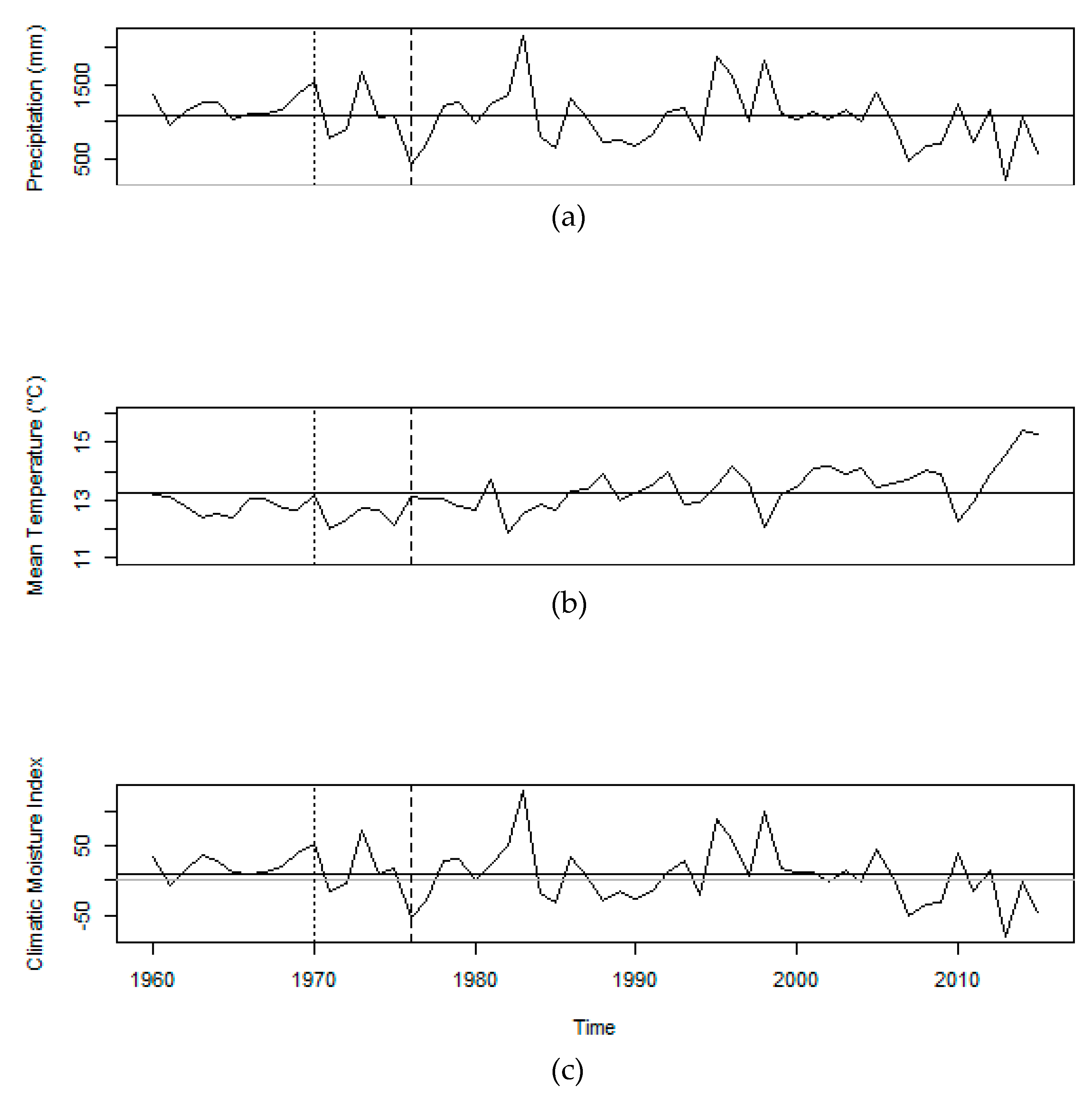
We downloaded the monthly weather data from the PRISM climate website based on the geographic location of the study site [45]. Variables obtained include monthly precipitation (PPT) (mm), minimum temperature, mean temperature, and maximum temperature (°C) from 1960–2015. Using these weather data, we calculated potential evapotranspiration (PET) and climatic moisture index (CMI) which involves subtracting PET from PPT [46]. During this period, the average annual precipitation was 1072 mm and the arid season occurred approximately from mid-May through the end of September (Figure 2) (R package “climatol”) (R version 3.5.1, The RStudio, Inc., Boston, MA, USA). The 30.2 value corresponds to the mean of the average daily maximum temperature of the hottest month (°C) and 1.9 corresponds to the mean of the average daily minimum temperature of the coldest month (°C). Annual variation in mean temperature (°C), precipitation (mm), and a dimensionless climatic moisture index (precipitation-evapotranspiration) from 1960 to 2015 is provided in Figure 3. For seasonality, precipitation and climatic moisture index were summed, while temperature was averaged over three-month periods.

2.4. Data Analysis

Quadratic mean diameter (QMD) and volume were calculated with Zhang’s equation [47] from the long-term plot inventories from 1975–2005. A split-plot analysis of variance with density in main plot and shrub removal in the subplot with age as the repeated measure was conducted with PROC GLM in SAS version 9.4 (SAS Institude Inc., Cary, NC, USA).
The raw ring width measurements were converted to ring-width indices (RWI) by detrending the individual series using a spline 67% of the series length with a 50% cutoff [48]. Treatment chronologies were computed using a robust (Biweight) mean for both the standard and residual (with autocorrelation removed) chronologies (dplR package, R) [48]. Descriptive statistics for each chronology were calculated using the R package “DetrendeR” for a common time interval of 1977–2011 [49]. These statistics include: mean ring width, mean correlation, expressed population signal (EPS), subsample signal strength (SSS), and the time interval during which SSS is greater than 0.85 [48,50].
To assess the long-term influence of climate on post-treatment radial growth, we looked at the period from 1977–2011 (35 years). The last five years (2012–2016) of growth were not included to eliminate the impacts of the 2012 Mill Fire. The residual chronologies produced by “dplR” were related to monthly and seasonal climate variables using the R program developed in Chhin et al. [51] over the 35-year period starting in April of the previous year (t–1) to August of the current growing year (t) (17-months). We included prior year climate in our analysis because previous studies have found ponderosa can have strong lagged effects of climate [30,33]. This particular R program has also been used in several other studies and is useful for analyzing multiple chronologies and climate variables at once, in addition to providing adjusted R2 values for the explanatory power of the individual models [33,52,53]. This model involves step-wise multiple regression with forward selection using the “StepAIC” function in R for selecting models with the lowest Akaike Information Criteria (AIC) to identify statistically significant (p < 0.05) relationships between monthly and/or seasonal climate variables and radial growth [51,54,55]. The residual chronologies were selected for the climate program because regression analysis assumes no autocorrelation. The climate variables used in this type of analysis are examined separately and included mean temperature (MET), precipitation (PPT), and climatic moisture index (CMI). We used partial regression coefficients (β) to rank the importance of climate predictor variables when the models produced more than one significant variable [51,56].
We calculated resistance indices for each year of the detrended treatment chronologies using the following formula [57,58]:
Resistance (Rt) = Dr/PreDr,
where Dr is defined as the performance during a disturbance and PreDr is the performance before a disturbance [57]. These indices were produced for each detrended chronology using the “res.comp” function in the R package “pointRes” calculated with four years pre-disturbance, a negative threshold of 20, and a series threshold of 75 [57,58]. PointRes treats each RWI as the “disturbance” and PreDr is the ring width indices of the previous four years’ growth. Lloret et al. [57] defines resistance as the “reversal of the reduction in ecological performance during disturbance”. Similar to Marques et al. [59], we correlated the resistance indices with the monthly climatic variables over the time period 1977–2011 (CMI, MET, and PPT). The correlation analysis was completed using the “dcc” function in the R package “bootRes” which is functionally identical to the popular Dendroclimatic program DendroClim2002 [60,61]. We used a correlation analysis between the resistance indices for each treatment and the monthly climatic variables from January through December. The correlation functions were computed with bootstrapped confidence intervals set to a significance level of 0.05.

3. Results

3.1. Treatment Effect on Growth and Chronology Statistics

The mean ring width (mm) over the common interval increased within each density treatment based on increasing shrub removal (V1 < V0.5 < V0) (Table 1). The 550 (V0) treatment had the largest mean ring width of all the groups (Table 1). Mean correlation for treatment chronologies during 1977–2011, ranged from 0.25 (1080 (V0)) to 0.45 (550 (V0)). In general, the EPS values were high, and only the 1080 (V1) and (V0) chronologies had EPS values lower than 0.85 (0.84 each). All treatment SSS values were above the 0.85 threshold for the common time period [50,62].
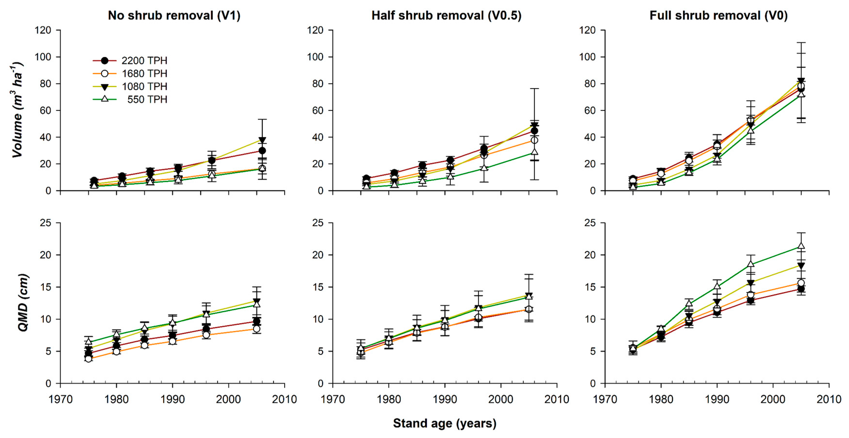
The response of the two stand characteristics, volume (m3 ha−1) and quadratic mean diameter (QMD) (cm), were highly significant to shrub removal, but not density (Figure 4; Table 2) over time. The full shrub removal (V0) treatments were significantly higher in both volume and QMD compared to the two treatments with a shrub presence. Lack of differences in interactions between density and shrub removal suggests an independency between these treatments on stand growth. Significant levels of age and age-associated interactions are detailed in Table 2; in particular, an interaction was significant for QMD between age and density with stand development. Annual trends for ring width indices (RWI) were similar between the different treatments (Figure 5).

3.2. Climate-Growth Relationships

For the multiple regression analysis, all treatments showed a significant response to each the three climate variables under consideration (Figure 6). Every treatment had a negative relationship to mean temperature in the spring and early summer of the current year (Figure 6a). The 1680 (V0) residual chronology was the only treatment with a positive seasonal relationship to mean temperature from December–February. There were no lagged effects of mean temperature on radial growth. Within each density treatment, the (V1) (no shrub removal) RWIs showed a weaker response to temperature compared to the other shrub treatments indicated by smaller adjusted R2 values.
Overall, precipitation at the beginning of the growing season for the current year had a positive relationship to radial growth (Figure 6b). April precipitation during the current growing season was positively related to all treatments with the exception of the 2200 (V0). The 2200 (V1) and (V0), 1680 (V1) and the 550 (V1) treatments also had positive responses to the current year’s May precipitation. The 2200 (V1) and 550 (V0) were the only treatments with a negative relationship to precipitation in August and September of the previous year (t–1), respectively. Precipitation was also positive for three treatments in February of the current year (t). Every (V0.5) shrub treatment was influenced by precipitation in October of the previous year. For the radial growth relationship to precipitation, the adjusted R2 values were lowest for all the (V0) shrub treatments, compared to the (V1) and (V0.5) of the same density. Compared to temperature, the explanatory power (R2) of the precipitation models within each density treatment was higher for the (V1) shrub groups, and lower for the (V0) groups. For the (V0.5) climate models, temperature R2 were higher or similar to precipitation values in the higher density treatments, and smaller in the two lowest densities.
In general, the explanatory power of the CMI models (Figure 6c) (R2) was higher compared to the precipitation models (Figure 6b) for each group. The exception is that growth response to precipitation was stronger than CMI in the 550 density (V0.5) and (V0) groups. For all (V0) groups, the temperature model (Figure 6a) had a better explanatory power for radial growth than precipitation or CMI as represented by the larger values for (R2), while the (V1) treatments were the opposite. Similar to precipitation, the adjusted R2 values for CMI and RWIs were the smallest within density treatments for the (V0) full shrub removal groups, with the exception of the 1080 TPH density where the (V0) was similar to the (V1) (Figure 6c). CMI in the three-month season March to May of the current growing year was positively related to radial growth for almost every treatment; 2200 (V0.5) was positive in only April, while 2200 (V0) was positive in April through June. While the regression model did show a positive relationship between the 1080 (V0.5) treatment and CMI in June to August of the current year, the p-value was greater than 0.05. All four of the two highest density treatments with a shrub presence had a significant positive relationship to current year CMI during the June, July, August season. Both the 550 density treatments with a shrub presence also had a positive relationship to current year June CMI. A positive response to January CMI was significant for 1680 (V1), 1080 (V0.5), and 550 (V1). The 1080 (V0.5) treatment also showed a positive relationship to previous year October CMI. Only 2200 (V1) and 1080 (V0) showed a negative response to CMI in the previous summer.

3.3. Treatment Effects on Resistance Correlation to Climate

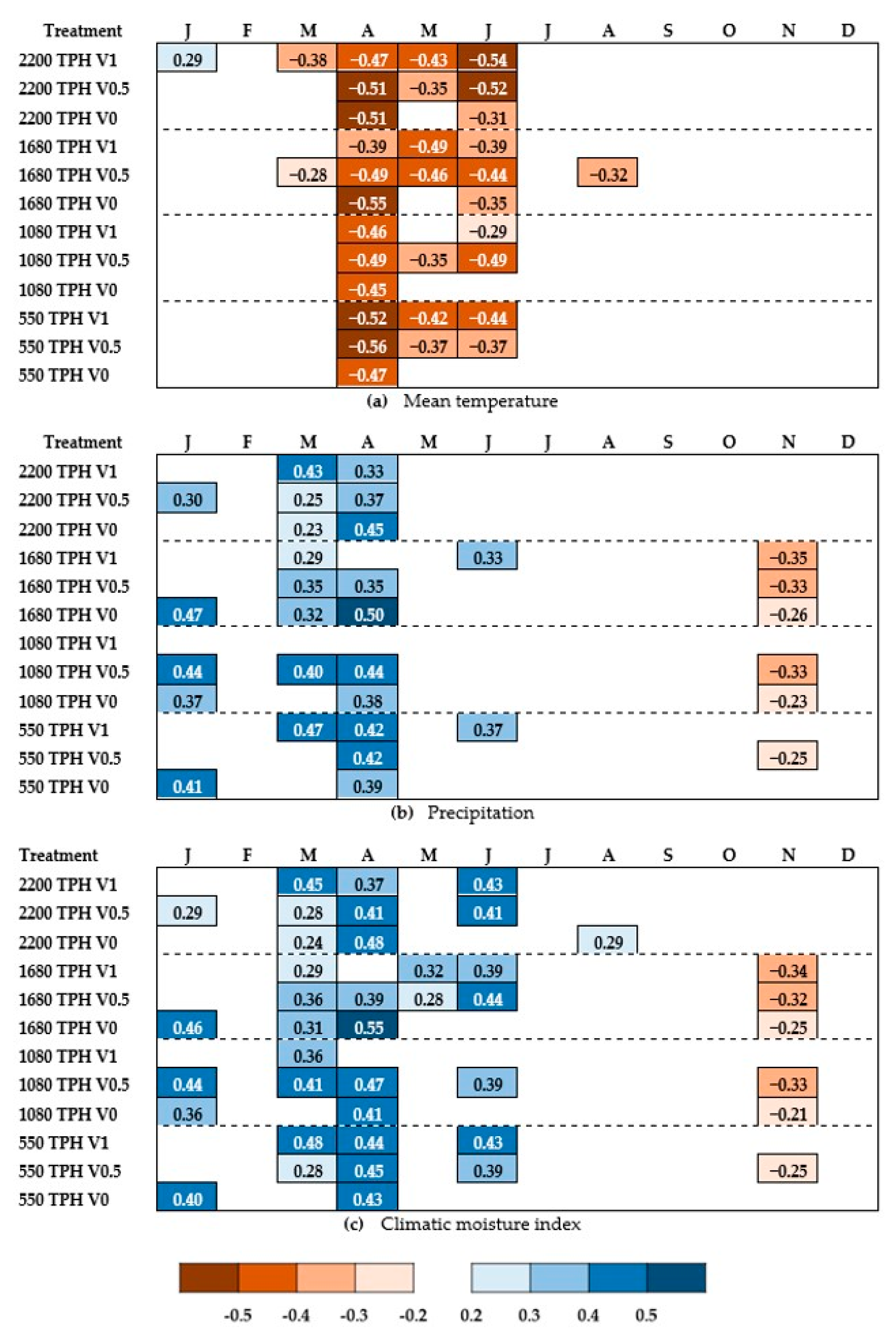
Values for significant Pearson correlation coefficients between monthly climate and resistance indices modelled by the bootstrapped correlation analysis are shown in Figure 7. Overall, we saw similar patterns as the regression analysis from Figure 6. In general, resistance appears to correlate more to climate variables in the spring and early summer from previous years. April is the month that appears to have the greatest impact on resistance, as it was significant for almost all treatment groups for each of the climate variables.
All treatment resistance indices had significant negative correlations to the mean temperature in April (Figure 7a) with larger Pearson coefficients than corresponding PPT (Figure 7b) and CMI (Figure 7c) during the same month. Treatments 1080 and 550 (V0) were the only groups with a single significant monthly correlation to MET. The only positive correlation to MET was in January for the 2200 (V1) treatment. All (V1) and (V0.5) shrub groups as well as the two highest density (V0) treatments were correlated to MET in June. May MET resistance correlation was also significant for all but one of the groups with a shrub component (1080 (V1)). Groups 2200 (V1), and 1680 (V0.5) resistance indices were correlated to March MET, and the latter group was the only treatment correlated to August.
Correlation between resistance indices and precipitation is presented in Figure 7b. All significant PPT coefficients beginning in January and ending in June were positively correlated to resistance. Group 1080 (V1) was the only treatment where resistance was not correlated to PPT during any month. January precipitation was significantly correlated to 2200 and 1080 (V0.5) groups as well as all (V0) treatments with the exception of the highest density. Precipitation in March was significant for the two highest densities (all shrub treatments) as well as the 1080 (V0.5) and 550 (V1) groups. All treatments, excluding the previously mentioned treatment and 1680 (V1) had positive correlation to April PPT. June PPT was correlated to 1680 and 550 (V1) treatments. November PPT was negatively correlated to all of the 1680 densities, the 1080 (V0.5) and (V0), and 550 (V0.5).
Resistance correlation coefficients were only negatively correlated to November CMI, all other significant correlations are positive (Figure 7c). The monthly CMI correlations for January, April, and November are virtually identical to PPT with similar Pearson coefficients. March CMI is significant for all treatments except for the two lowest density (V0) groups. Both 1680 (V1) and (V0.5) had positive correlation to May CMI. June CMI (Figure 7c) resistance correlations were significant for the same treatments with significant May MET correlations (Figure 7a). The density control treatment 2200 (V0) was the only treatment with a correlation between resistance and CMI in August.

4. Discussion

This study provides long-term evidence that moisture availability is an overriding factor for plant growth in temperate regions of Mediterranean climate [63]. We have shown that without substantial shrub removal treatments when ponderosa pine plantations are young, the growth and vigor of trees will have continued detrimental impacts decades later [19,47]. Tree-ring analysis only allows for the inference of physiological responses to climate. Long-term studies on second-growth ponderosa pine have shown that thinning treatments improve physiological processes, which include, but are not limited to, higher predawn and midday water potential, resin production, phloem thickness, stomatal conductance, radial growth and net photosynthetic rate [64,65]. Although temperature showed a significant correlation with radial growth, it is possible that its effect on growth and resistance was due to influencing soil moisture, as the seasonal and monthly variables had similar timing to the CMI modeling (Figure 6a,c). Our discussion will focus on how stand density manipulation and shrub control affect the long-term relationships of radial growth and climate.

4.1. Treatment Effect on Long-Term Relationships between Growth and Climate

All treatments, regardless of density or shrub removal, had a significantly negative radial growth response to current growing year (t) spring temperature (Figure 6a). Johnson et al. [33] also found a negative association with the same-year growing season temperature for old-growth ponderosa pine in California’s Sierra Nevada. However, that same study also saw a lagged negative association to previous May mean temperature while our Trough Springs plantation had no lagged response. Radial growth for dry sites have been shown to be more reliant on current year climate conditions (t) compared to humid sites, which are often more dependent on lagged conditions (t–1) [66]. Ponderosa pine co-occurring with western juniper at multiple sites in southern Oregon was also negatively associated with June temperature during the current growing season [40]. The negative relationship identified in our study may be due to early spring temperature controlling both timing of snowmelt and evapotranspiration, which determines the amount of water availability for vegetation. Early high temperature means snow melts faster and PET will be higher; water availability will be lower in the late growing seasons. Additionally, the shallow gravel soil with a low water-holding capacity is another indication of low water availability in the soil profile at this site. Therefore, less radial growth is expected. Within each density, sensitivity to MET was lowest for all groups with no shrub removal (V1) (explanatory power of the adjusted R2) compared to the other treatment groups likely because understory manzanita helped maintain cooler soil temperatures by blocking direct sunshine on ground. A meta-analysis on the effects of thinning on forest soils across multiple continents, found that thinning often results in increased soil temperature and respiration Zhang et al. [67], which supports the temperature trends in our results. For the full shrub removal groups (V0), the explanatory power (R2) was stronger for the MET model (Figure 6a) compared to both the PPT (Figure 6b) and CMI (Figure 6c) models, indicating greater sensitivity to temperature compared to moisture availability. Thinned Pinus nigra in Spain was also more sensitive to temperature while sensitivity to precipitation was reduced [68]. Temperature was also shown to be the primary influence on growth for Picea abies in the Italian Alps [69]. Within the same density treatments, MET still had a stronger influence in the half shrub removal groups (V0.5) compared to full shrub removal (V0).
Precipitation during the current year growing season often has a significant positive influence on radial growth for multiple tree species across varying site conditions [33,51,53,70,71]. While the precipitation modelling (Figure 6b) showed similar trends in adjusted R2 values and positive springtime relationships to RWI as CMI (Figure 6c), none of the treatments had seasonal (three-month) relationship to PPT, only monthly responses. Comparatively, the radial relationships between both temperature (Figure 6a) and CMI (Figure 6c) had at least one significant seasonal variable identified by the model. For PPT (Figure 6b), current year April and/or May were usually the primary or singular monthly variables influencing growth, indicating that radial growth benefits from rainfall occurring at the start of the growing season, regardless of treatment. Comparatively, for mature ponderosa in the Sierra Nevada mountains, Johnson et al. [33] found a strong lagged response to precipitation with October-December (t–1) and May (t–1) having a primary and secondary influence on growth (respectively), while February through April (t) was only tertiary. Many factors may cause these differences between two studies, including elevation, climate, soil type and depth, tree age, and analysis periods. As summer precipitation at Trough Springs was essentially nonexistent, it was not surprising that there were no relationships between RWI and PPT after May (t). An unexpected observation was the limited response to winter precipitation, with only three treatments having a significant response, all with an understory component across different densities. Other dendroclimatology reports for montane ponderosa pine in California have identified positive relationships to winter snowpack [30,33,35]. The extremely high drainage and low water holding capacity of these soils may have contributed to the limited response at this site.
Previous research found that ponderosa pine over a wide geographic range is often more sensitive to moisture than to temperature [31,36,40,72]. By using climatic moisture index, we can incorporate both temperature and moisture into a single model. Despite rare summer precipitation events, CMI values were always negative during the June–August (t) season from 1977–2011. While we have not directly studied the rooting characteristics and water utilization at the Trough Springs site, many California forests are adapted to survive summer droughts as long as intraspecific competition is low [21]. The nonexistent or limited effect of summer drought stress on the two lowest density treatments (both with/and without shrubs) further supports intraspecific competition among ponderosa pine having a greater impact than competition with manzanita (Figure 6c). The regression analysis between RWI and CMI indicated that the two highest densities with manzanita presence are stressed by the summer moisture deficits and benefit from spring CMI, while complete shrub removal and lower pine densities are only affected by spring moisture availability (Figure 6c). For the CMI models, moisture availability during the summer season (June through August) is the primary driver of radial growth (i.e., highest β coefficient) for treatments with the highest competition. Comparatively, summer CMI was either not significant, or only a secondary variable related to radial growth for treatments with less competition (Figure 6c). In our CMI model, the seasonal responses of the (V1) and (V0) were very similar to one another within the same densities supporting previous conclusions that when manzanita presence is severe, only significant reductions in crown cover will benefit pine growth [19,47]. One potential explanation as to why summer drought stress (t) was only detrimental to the subplots with competing shrub presence is that manzanita species have shown to be better adapted to acquiring water from bedrock and moisture depleted soils than pines [26,73]. Zones of weathered bedrock are an important source of water for plants during dry California summers and at a site in the Sierra Nevada, weathered bedrock was responsible for providing water to forest vegetation up to 70% during the growing season [14]. While both ponderosa pine and manzanita species are adapted to seasonal periods of drought, the mechanisms of adaptation are different. When ponderosa pine and greenleaf manzanita (Arctostaphylos patula) seedlings were exposed to differing levels of moisture stress, the results indicated that manzanita was better able to extract water from moisture-limited soils while ponderosa pine seedlings were able tolerate water loss by rapidly closing stomata and, therefore, reducing water loss through transpiration [26]. Seedling studies with varying density levels of greenleaf manzanita competition with ponderosa pine showed that soil moisture depletion was significantly lower for pine without manzanita presence than soils in mixed stands with consistent light availability [18]. Our results indicate that ponderosa pine suffering from both intra- and inter-specific competition are less able to tolerate summer drought.
The differences in response to CMI between the two extremes in our treatment groups (2200 TPH (V1) and 550 TPH (V0)) support our hypothesis that the treatments with the highest competition would be more sensitive to climate compared to lowest competition (Figure 6c). An unexpected result was the similarity between the 2200 (V0) and 550 (V0) TPH groups, particularly for the response to CMI. This indicates that the climatic sensitivity is more dependent on shrub removal status, than density. However, the monthly delay (April–May–June compared to March–April–May) for the seasonal relationship for 2200 (V0) group does stand out, and further supports the sensitivity to summer drought stress for higher density stands. Of these two groups, the explanatory power of the temperature model was stronger for 2200 TPH. This may be a more important factor for climate sensitivity based on multiple climate simulation models for northern California with increased warming during summer while precipitation regimes remain similar or with slight declines [16,17]. The significantly larger growth of the 550 TPH treatment should also be considered as an important indication of overall tree health [47].

4.2. Treatment Effects on Tree Resistance Response to Climate

As far as we are aware, no other studies of ponderosa pine have performed correlation analysis between resistance indices and monthly climate variables as it was a novel approach for studying European riparian forest resilience to climate change [59] (Figure 7). Similar studies have shown that thinning improves resilience variables (i.e., resistance, resilience, and recovery) to drought for multiple conifer species in Europe [7,8,9], and the United States [10,74]. Analysis of specific droughts across a wide geographic and climatic range in the United States showed that resistance and resilience were improved for both Pinus ponderosa and Pinus resinosa at lower densities [10]. Mixed results in drought response to thinning have been observed [66,75]. After first, recent, and heavy thinning, the drought recovery for Pinus sylvestris radial growth was improved in Germany [75]. These benefits to radial growth, however, either declined or became negative compared to control stands when the amount of time since last thinning increased [75]. Heavily thinned Norway spruce growing in humid and dry sites in Belgium showed periods of growth reduction when the climate response modeling was comparatively stable; which may have been due to air pollution becoming the limiting factor following thinning [66]. Overall, the monthly trends we saw for correlation between climate and resistance (Figure 7) were similar to the multiple regression analysis for RWI (Figure 6) with spring having an important impact. The differences were complex; therefore, we will discuss trends seen across similar groups as well as the treatment group extremes. As resistance in this study is the ratio between current year radial growth and growth four years prior, the coefficients between resistance and climate indicate the prior year’s climate variables that influence the ability of trees to tolerate drought events [57,58,59].
The negative correlation between resistance indices for every treatment group and April mean temperature (MET) indicates that higher temperatures at the beginning of preceding years’ growing season have continued detrimental impacts on growth for all trees at this site, which stays in the same line of argument for available soil moisture (Figure 7a). It was expected that the damaging effects of spring temperature would be more prevalent for the highest densities and groups with shrub components as physiological processes are hindered in unthinned stands [20,64,65]. The correlation analysis of resistance indices did result in a larger number of months with significant correlations to MET for the higher densities, and especially for the treatments that had shrub competition. The greater number of positive significant coefficients during the first months of the year between PPT (Figure 7b) and CMI (Figure 7c) and resistance in treatment groups with higher competition suggests that they are more dependent on previous growing season’s moisture availability compared to the more heavily treated groups. Greater sensitivity to previous years’ moisture availability is important because multi-year droughts are occurring more frequently in California and are likely to continue to do so. While the negative response to PPT and CMI for several groups in wetter Novembers was unexpected, other studies have seen similar RWI responses to autumn and winter precipitation [52,53]. Although the regression analysis (Figure 6) did not show stronger responses of radial growth to the previous year’s weather conditions, the results from the resistance correlation analysis (Figure 7) support the importance of previous resource availability on a tree’s ability to overcome drought [32,33,34,36]. Overall, heavy thinning combined with complete shrub removal resulted in ponderosa pine resistance being less sensitive to climate conditions.

4.3. Study Limitations and Future Research Recommendations

Due to the Mill fire causing mortality throughout the study site, cores were only collected from live trees, potentially limiting our sample variation. However, the retrospective tree ring analysis allowed us to only examine years before the disturbance. Another limitation of this study is that the analysis only included stand models and did not consider individual tree variability. Therefore, future research could investigate individual tree growth response using individual non-linear models for improved resolution of growth as utilized by Girona et al. [76]. As application of the methodology described in this paper is novel with respect to managed ponderosa pine plantations in California, further research can be expanded to additional locations across a range of site qualities. Additionally, since the relationship between competition and response to climate has been shown to vary across different site aridity and focal species [1,11,77], future studies for different tree species will provide a greater understanding of forest response to climate change.

5. Conclusions

On a poor-quality site with low water-holding capacity and high runoff, the effects of density and shrub removal treatments persist decades after treatment. Similar to what Oliver [19] concluded for the Trough Springs ridge plantation we found that the presence of shrub cover had a persistent influence on ponderosa pine. In the 35 years following treatment, all treatments, including the control, significantly responded to spring temperature and precipitation during the current growing season. Higher spring temperature reduced radial growth while greater precipitation and moisture availability benefited growth. The results indicate that higher density plantations with shrub presence are more stressed due to summer droughts. Our study supports existing information that understory competition removal and lower plantation densities increase stand growth for sites with a strong understory component. Controlling shrubs will result in a more successful reforestation and likely reduce understory fuel loads and ladder fuels. When combining with lower tree density, it will significantly enhance tree growth rate, stand development, and resistance to climate change.

Author Contributions

K.F. and J.Z. conceived and implemented the study; K.F. managed the fieldwork; K.F. performed the labwork; K.F. and J.Z. analyzed the data; K.F. wrote the paper with input from J.Z.; project supervision and funding acquisition by J.Z.

Funding

This research received no external funding.

Acknowledgments

This study would not be possible without William Oliver; who designed the original study, administered the installation and was responsible for early data collection. Thanks to everyone who has contributed to data collection over the years, as well as special thanks to Billy Bullard and Colin Pryor who helped with increment core collection. Comments from Brianna Finley and two anonymous reviewers are greatly appreciated. Use of trade names in this paper does not constitute endorsement by the United States Forest Service.

Conflicts of Interest

The authors declare no conflict of interest.

References

  1. Gleason, K.E.; Bradford, J.B.; Bottero, A.; D’Amato, A.W.; Fraver, S.; Palik, B.J.; Battaglia, M.A.; Iverson, L.; Kenefic, L.; Kern, C.C. Competition amplifies drought stress in forests across broad climatic and compositional gradients. Ecosphere 2017, 8. [Google Scholar] [CrossRef] [Green Version]
  2. Allen, C.D.; Macalady, A.K.; Chenchouni, H.; Bachelet, D.; McDowell, N.; Vennetier, M.; Kitzberger, T.; Rigling, A.; Breshears, D.D.; Hogg, E.H.; et al. A global overview of drought and heat-induced tree mortality reveals emerging climate change risks for forests. For. Ecol. Manag. 2010, 259, 660–684. [Google Scholar] [CrossRef] [Green Version]
  3. Dai, A.G. Drought under global warming: A review. Wiley Interdiscip. Rev. Clim. Chang. 2011, 2, 45–65. [Google Scholar] [CrossRef]
  4. Nolan, R.H.; Drew, D.M.; O’Grady, A.P.; Pinkard, E.A.; Paul, K.; Roxburgh, S.H.; Mitchell, P.J.; Bruce, J.; Battaglia, M.; Ramp, D. Safeguarding reforestation efforts against changes in climate and disturbance regimes. For. Ecol. Manag. 2018, 424, 458–467. [Google Scholar] [CrossRef]
  5. Clark, J.S.; Iverson, L.; Woodall, C.W.; Allen, C.D.; Bell, D.M.; Bragg, D.C.; D’Amato, A.W.; Davis, F.W.; Hersh, M.H.; Ibanez, I.; et al. The impacts of increasing drought on forest dynamics, structure, and biodiversity in the United States. Glob. Chang. Biol. 2016, 22, 2329–2352. [Google Scholar] [CrossRef] [PubMed] [Green Version]
  6. Diaconu, D.; Kahle, H.P.; Spiecker, H. Thinning increases drought tolerance of European beech: A case study on two forested slopes on opposite sides of a valley. Eur. J. For. Res. 2017, 136, 319–328. [Google Scholar] [CrossRef]
  7. Kohler, M.; Sohn, J.; Nagele, G.; Bauhus, J. Can drought tolerance of Norway spruce (Picea abies (L.) Karst.) be increased through thinning? Eur. J. For. Res. 2010, 129, 1109–1118. [Google Scholar] [CrossRef]
  8. Guillemot, J.; Klein, E.K.; Davi, H.; Courbet, F. The effects of thinning intensity and tree size on the growth response to annual climate in Cedrus atlantica: A linear mixed modeling approach. Ann. For. Sci. 2015, 72, 651–663. [Google Scholar] [CrossRef]
  9. Navarro-Cerrillo, R.M.; Sanchez-Salguero, R.; Rodriguez, C.; Lazo, J.D.; Moreno-Rojas, J.M.; Palacios-Rodriguez, G.; Camarero, J.J. Is thinning an alternative when trees could die in response to drought? The case of planted Pinus nigra and P. Sylvestris stands in southern Spain. For. Ecol. Manag. 2019, 433, 313–324. [Google Scholar] [CrossRef]
  10. Bottero, A.; D’Amato, A.W.; Palik, B.J.; Bradford, J.B.; Fraver, S.; Battaglia, M.A.; Asherin, L.A. Density-dependent vulnerability of forest ecosystems to drought. J. Appl. Ecol. 2017, 54, 1605–1614. [Google Scholar] [CrossRef]
  11. Keyser, T.L.; Brown, P.M. Drought response of upland oak (Quercus L.) species in Appalachian hardwood forests of the southeastern USA. Ann. For. Sci. 2016, 73, 971–986. [Google Scholar] [CrossRef]
  12. Berner, L.T.; Law, B.E.; Meddens, A.J.H.; Hicke, J.A. Tree mortality from fires, bark beetles, and timber harvest during a hot and dry decade in the western United States (2003–2012). Environ. Res. Lett. 2017, 12. [Google Scholar] [CrossRef]
  13. North, M.P.; Stevens, J.T.; Greene, D.F.; Coppoletta, M.; Knapp, E.E.; Latimer, A.M.; Restaino, C.M.; Tompkins, R.E.; Welch, K.R.; York, R.A.; et al. Tamm Review: Reforestation for resilience in dry western US forests. For. Ecol. Manag. 2019, 432, 209–224. [Google Scholar] [CrossRef]
  14. Witty, J.H.; Graham, R.C.; Hubbert, K.R.; Doolittle, J.A.; Wald, J.A. Contributions of water supply from the weathered bedrock zone to forest soil quality. Geoderma 2003, 114, 389–400. [Google Scholar] [CrossRef]
  15. Hubbert, K.R.; Beyers, J.L.; Graham, R.C. Roles of weathered bedrock and soil in seasonal water relations of Pinus Jeffreyi and Arctostaphylos patula. Can. J. For. Res. 2001, 31, 1947–1957. [Google Scholar] [CrossRef]
  16. Hayhoe, K.; Cayan, D.; Field, C.B.; Frumhoff, P.C.; Maurer, E.P.; Miller, N.L.; Moser, S.C.; Schneider, S.H.; Cahill, K.N.; Cleland, E.E.; et al. Emissions pathways, climate change, and impacts on California. Proc. Natl. Acad. Sci. USA 2004, 101, 12422–12427. [Google Scholar] [CrossRef] [PubMed] [Green Version]
  17. Cayan, D.R.; Maurer, E.P.; Dettinger, M.D.; Tyree, M.; Hayhoe, K. Climate change scenarios for the California region. Clim. Chang. 2008, 87, S21–S42. [Google Scholar] [CrossRef]
  18. Shainsky, L.J.; Radosevich, S.R. Growth and water relations of Pinus ponderosa seedlings in competitive regimes with Arctostaphylos patula seedlings. J. Appl. Ecol. 1986, 23, 957–966. [Google Scholar] [CrossRef]
  19. Oliver, W.W. Brush Reduces Growth of Thinned Ponderosa Pine in Northern California. 1984; Usda Forest Service Pacific Southwest Research Station Research Paper. Available online: https://www.fs.usda.gov/treesearch/pubs/28833 (accessed on 25 April 2019).
  20. Powers, R.F.; Reynolds, P.E. Ten-year responses of ponderosa pine plantations to repeated vegetation and nutrient control along an environmental gradient. Can. J. For. Res. 1999, 29, 1027–1038. [Google Scholar] [CrossRef]
  21. Zhang, J.W.; Powers, R.F.; Oliver, W.W.; Young, D.H. Response of ponderosa pine plantations to competing vegetation control in Northern California, USA: A meta-analysis. Forestry 2013, 86, 3–11. [Google Scholar] [CrossRef]
  22. Zhang, J.W.; Busse, M.D.; Young, D.H.; Fiddler, G.O.; Sherlock, J.W.; TenPas, J.D. Aboveground biomass responses to organic matter removal, soil compaction, and competing vegetation control on 20-year mixed conifer plantations in California. For. Ecol. Manag. 2017, 401, 341–353. [Google Scholar] [CrossRef]
  23. Zhang, J.W.; Ritchie, M.W.; Maguire, D.A.; Oliver, W.W. Thinning ponderosa pine (Pinus ponderosa) stands reduces mortality while maintaining stand productivity. Can. J. For. Res. 2013, 43, 311–320. [Google Scholar] [CrossRef]
  24. Girona, M.M.; Morin, H.; Lussier, J.-M.; Ruel, J.-C. Post-cutting mortality following experimental silvicultural treatments in unmanaged Boreal forest stsands. Front. For. Glob. Chang. 2019, 2. [Google Scholar] [CrossRef]
  25. White, D.E.; Newton, M. Competitive interactions of whiteleaf manzanita, herbs, Douglas-fir, and ponderosa pine in southwest Oregon. Can. J. For. Res. 1989, 19, 232–238. [Google Scholar] [CrossRef]
  26. Anderson, P.D.; Helms, J.A. Tissue water relations of Pinus ponderosa and Arctostaphylos patula exposed to various levels of soil-moisture depletion. Can. J. For. Res. 1994, 24, 1495–1502. [Google Scholar] [CrossRef]
  27. Newton, M.; Cole, E.C. Twenty-six-year response of ponderosa pine and Douglas-fir plantations to woody competitor density in treated stands of madrone and whiteleaf manzanita. For. Ecol. Manag. 2008, 256, 410–420. [Google Scholar] [CrossRef]
  28. McDowell, N.; Pockman, W.T.; Allen, C.D.; Breshears, D.D.; Cobb, N.; Kolb, T.; Plaut, J.; Sperry, J.; West, A.; Williams, D.G.; et al. Mechanisms of plant survival and mortality during drought: Why do some plants survive while others succumb to drought? New Phytol. 2008, 178, 719–739. [Google Scholar] [CrossRef] [PubMed]
  29. Adams, H.D.; Kolb, T.E. Tree growth response to drought and temperature in a mountain landscape in northern Arizona, USA. J. Biogeogr. 2005, 32, 1629–1640. [Google Scholar] [CrossRef]
  30. Aubry-Kientz, M.; Moran, E.V. Climate impacts on tree growth in the Sierra Nevada. Forests 2017, 8, 414. [Google Scholar] [CrossRef]
  31. Carnwath, G.C.; Peterson, D.W.; Nelson, C.R. Effect of crown class and habitat type on climate-growth relationships of ponderosa pine and Douglas-fir. For. Ecol. Manag. 2012, 285, 44–52. [Google Scholar] [CrossRef]
  32. Dannenberg, M.P.; Wise, E.K. Seasonal climate signals from multiple tree ring metrics: A case study of Pinus ponderosa in the upper Columbia River Basin. J. Geophys. Res. Biogeosci. 2016, 121, 1178–1189. [Google Scholar] [CrossRef]
  33. Johnson, C.; Chhin, S.; Zhang, J. Effects of climate on competitive dynamics in mixed conifer forests of the Sierra Nevada. For. Ecol. Manag. 2017, 394, 1–12. [Google Scholar] [CrossRef]
  34. Kusnierczyk, E.R.; Ettl, G.J. Growth response of ponderosa pine (Pinus ponderosa) to climate in the eastern Cascade Mountains, Washington, USA: Implications for climatic change. Ecoscience 2002, 9, 544–551. [Google Scholar] [CrossRef]
  35. McCullough, I.M.; Davis, F.W.; Williams, A.P. A range of possibilities: Assessing geographic variation in climate sensitivity of ponderosa pine using tree rings. For. Ecol. Manag. 2017, 402, 223–233. [Google Scholar] [CrossRef]
  36. Pettit, J.; Derose, R.; Long, J. Climatic drivers of ponderosa pine growth in central Idaho. Tree Ring Res. 2018, 74, 172–184. [Google Scholar] [CrossRef]
  37. Soule, P.T.; Knapp, P.A. Radial Growth and Increased Water-Use Efficiency for Ponderosa Pine Trees in Three Regions in the Western United States. Prof. Geogr. 2011, 63, 379–391. [Google Scholar] [CrossRef] [Green Version]
  38. Bigelow, S.W.; Papaik, M.J.; Caum, C.; North, M.P. Faster growth in warmer winters for large trees in a Mediterranean-climate ecosystem. Clim. Chang. 2014, 123, 215–224. [Google Scholar] [CrossRef]
  39. Knapp, P.A.; Soule, P.T. Increasing water-use efficiency and age-specific growth responses of old-growth ponderosa pine trees in the Northern Rockies. Glob. Chang. Biol. 2011, 17, 631–641. [Google Scholar] [CrossRef]
  40. Knutson, K.C.; Pyke, D.A. Western juniper and ponderosa pine ecotonal climate-growth relationships across landscape gradients in southern Oregon. Can. J. For. Res. 2008, 38, 3021–3032. [Google Scholar] [CrossRef]
  41. Speer, J.H. Fundamentals of Tree-Ring Research; University of Arizona Press: Tucscon, AZ, USA, 2010. [Google Scholar]
  42. Yamaguchi, D.K. A simple method for cross-dating increment cores from living trees. Can. J. For. Res. 1991, 21, 414–416. [Google Scholar] [CrossRef]
  43. Larsson, L. CooRecorder and Cdendro Programs of the CooRecorder/CdendroPackage, 8.1.1; Cybis: McLean, VA, USA, 2015. [Google Scholar]
  44. Grissino-Mayer, H.D. Evaluating Crossdating Accuracy: A manual and tutorial for the computer program COFECHA. Tree Ring Res. 2001, 57, 205–221. [Google Scholar]
  45. PRISM Climate Group. Available online: http://prism.oregonstate.edu (accessed on 25 April 2019).
  46. Hogg, E.H. Temporal scaling of moisture and the forest-grassland boundary in western Canada. Agric For. Meteorol. 1997, 84, 115–122. [Google Scholar] [CrossRef] [Green Version]
  47. Zhang, J.W.; Oliver, W.W.; Busse, M.D. Growth and development of ponderosa pine on sites of contrasting productivities: Relative importance of stand density and shrub competition effects. Can. J. For. Res. 2006, 36, 2426–2438. [Google Scholar] [CrossRef]
  48. Bunn, A.G. A dendrochronology program library in R (dplR). Dendrochronologia 2008, 26, 115–124. [Google Scholar] [CrossRef]
  49. Campelo, F.; Garcia-Gonzalez, I.; Nabais, C. detrendeR—A Graphical User Interface to process and visualize tree-ring data using R. Dendrochronologia 2012, 30, 57–60. [Google Scholar] [CrossRef]
  50. Wigley, T.M.L.; Briffa, K.R.; Jones, P.D. On the average value of correlated time-series, with applications in dendroclimatology and hydrometeorology. J. Clim. Appl. Meteorol. 1984, 23, 201–213. [Google Scholar] [CrossRef]
  51. Chhin, S.; Hogg, E.; Lieffers, V.; Huang, S. Potential effects of climate change on the growth of lodgepole pine across diameter size classes and ecological regions. For. Ecol. Manag. 2008, 256, 1692–1703. [Google Scholar] [CrossRef]
  52. Chhin, S.; Hogg, E.; Lieffers, V.; Huang, S. Growth-climate relationships vary with height along the stem in lodgepole pine. Tree Physiol. 2010, 30, 335–345. [Google Scholar] [CrossRef] [Green Version]
  53. Chhin, S.; O’Brien, J. Dendroclimatic analysis of red pine affected by Diplodia shoot blight in different latitudinal regions in Michigan. Can. J. For. Res. 2015, 45, 1757–1767. [Google Scholar] [CrossRef]
  54. Venables, W.N.; Ripley, B.D. Modern Applied Statistics with S., 4th ed.; Springer: New York, NY, USA, 2002. [Google Scholar]
  55. Burnham, K.P.; Anderson, D.R. Model Selection and Multimodel Inference: A Practical Information-Theoretic Approach; Springer-Verlag: New York, NY, USA, 2002. [Google Scholar]
  56. Zar, J.H. Biostatistical Analysis, 4th ed.; Prentice Hall: Upper Saddle River, NJ, USA, 1999. [Google Scholar]
  57. Lloret, F.; Keeling, E.G.; Sala, A. Components of tree resilience: Effects of successive low-growth episodes in old ponderosa pine forests. Oikos 2011, 120, 1909–1920. [Google Scholar] [CrossRef]
  58. van der Maaten-Theunissen, M.; van der Maaten, E.; Bouriaud, O. pointRes: An R package to analyze pointer years and components of resilience. Dendrochronologia 2015, 35, 34–38. [Google Scholar] [CrossRef]
  59. Marques, I.G.; Campelo, F.; Rivaes, R.; Albuquerque, A.; Ferreira, M.T.; Rodriguez-Gonzalez, P.M. Tree rings reveal long-term changes in growth resilience in Southern European riparian forests. Dendrochronologia 2018, 52, 167–176. [Google Scholar] [CrossRef]
  60. Zang, C.; Biondi, F. Dendroclimatic calibration in R: The bootRes package for response and correlation function analysis. Dendrochronologia 2013, 31, 68–74. [Google Scholar] [CrossRef]
  61. Biondi, F.; Waikul, K. DENDROCLIM2002: A C++ program for statistical calibration of climate signals in tree-ring chronologies. Comput. Geosci. 2004, 30, 303–311. [Google Scholar] [CrossRef]
  62. Buras, A. A comment on the expressed population signal. Dendrochronologia 2017, 44, 130–132. [Google Scholar] [CrossRef]
  63. Powers, R.F.; Ferrell, G.F. Moisture, nutrient, and insect constraints plantation growth: The “Garden of Eden” study. N. Z. J. For. Sci. 1996, 26, 126–144. [Google Scholar]
  64. Kolb, T.E.; Holmberg, K.M.; Wagner, M.R.; Stone, J.E. Regulation of ponderosa pine foliar physiology and insect resistance mechanisms by basal area treatments. Tree Physiol. 1998, 18, 375–381. [Google Scholar] [CrossRef] [Green Version]
  65. Sala, A.; Peters, G.D.; McIntyre, L.R.; Harrington, M.G. Physiological responses of ponderosa pine in western Montana to thinning, prescribed fire and burning season. Tree Physiol. 2005, 25, 339–348. [Google Scholar] [CrossRef] [Green Version]
  66. Laurent, M.; Antoine, N.; Joel, G. Effects of different thinning intensities on drought response in Norway spruce (Picea abies (L.) Karst.). For. Ecol. Manag. 2003, 183, 47–60. [Google Scholar] [CrossRef]
  67. Zhang, X.Z.; Guan, D.X.; Li, W.B.; Sun, D.; Jin, C.J.; Yuan, F.H.; Wang, A.Z.; Wu, J.B. The effects of forest thinning on soil carbon stocks and dynamics: A meta-analysis. For. Ecol. Manag. 2018, 429, 36–43. [Google Scholar] [CrossRef]
  68. Martin-Benito, D.; Del Rio, M.; Heinrich, I.; Helle, G.; Canellas, I. Response of climate-growth relationships and water use efficiency to thinning in a Pinus nigra afforestation. For. Ecol. Manag. 2010, 259, 967–975. [Google Scholar] [CrossRef]
  69. Castagneri, D.; Nola, P.; Cherubini, P.; Motta, R. Temporal variability of size-growth relationships in a Norway spruce forest: The influences of stand structure, logging, and climate. Can. J. For. Res. 2012, 42, 550–560. [Google Scholar] [CrossRef]
  70. Wang, X.C.; Pederson, N.; Chen, Z.J.; Lawton, K.; Zhu, C.; Han, S.J. Recent rising temperatures drive younger and southern Korean pine growth decline. Sci. Total Environ. 2019, 649, 1105–1116. [Google Scholar] [CrossRef]
  71. Helama, S.; Salminen, H.; Timonen, M.; Varmola, M. Dendroclimatological analysis of seeded and thinned Scots pine (Pinus sylvestris L.) stands at the coniferous timberline. New For. 2008, 35, 267–284. [Google Scholar] [CrossRef]
  72. Evans, M.E.K.; Falk, D.A.; Arizpe, A.; Swetnam, T.L.; Babst, F.; Holsinger, K.E. Fusing tree-ring and forest inventory data to infer influences on tree growth. Ecosphere 2017, 8. [Google Scholar] [CrossRef]
  73. Zwieniecki, M.A.; Newton, M. Seasonal pattern of water depletion from soil-rock profiles in a Mediterranean climate southwestern Oregon. Can. J. For. Res. 1996, 26, 1346–1352. [Google Scholar] [CrossRef]
  74. Magruder, M.; Chhin, S.; Palik, B.; Bradford, J. Thinning increases climatic resilience of red pine. Can. J. For. Res. 2013, 43, 878–889. [Google Scholar] [CrossRef]
  75. Sohn, J.A.; Hartig, F.; Kohler, M.; Huss, J.; Bauhus, J. Heavy and frequent thinning promotes drought adaptation in Pinus sylvestris forests. Ecol. Appl. 2016, 26, 2190–2205. [Google Scholar] [CrossRef]
  76. Girona, M.M.; Rossi, S.; Lussier, J.M.; Walsh, D.; Morin, H. Understanding tree growth responses after partial cuttings: A new approach. PLoS ONE 2017, 12. [Google Scholar] [CrossRef]
  77. Clark, J.S.; Bell, D.M.; Kwit, M.C.; Zhu, K. Competition-interaction landscapes for the joint response of forests to climate change. Glob. Chang. Biol. 2014, 20, 1979–1991. [Google Scholar] [CrossRef] [PubMed]
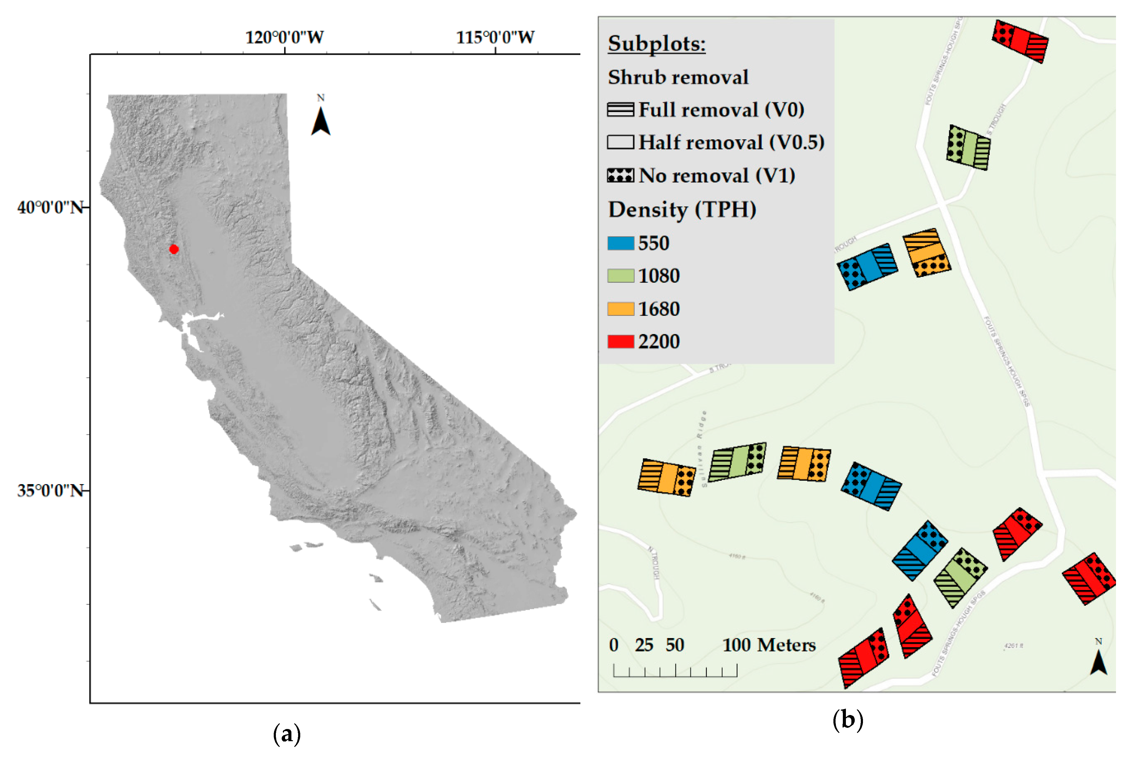
Figure 1. (a) Trough Springs plantation location in the north Coast Range of California (red); (b) 14 ponderosa pine research plots representing four densities (2200 TPH (control), 1680 TPH, 1080 TPH, and 550 TPH) and three shrub removal subplots: full shrub removal (V0); half shrub removal (V0.5); and no shrub removal (V1).
Forests 10 00477 g001
Figure 2. Walter–Lieth climate diagram for the Trough Spring study site (1285 m) from 1960–2015.
Forests 10 00477 g002
Figure 3. Annual variability and long-term trends in climate variables. (a) precipitation (mm); (b) mean temperature (°C); (c) climatic moisture index. Solid, dark horizontal lines represent mean values for each climatic variable for the time from 1960–2015. Vertical lines represent the years the study was treated (dotted is year thinned from below, dashed is year of shrub treatment). Precipitation and climatic moisture index are the total amounts for each year while temperature is the yearly average.
Forests 10 00477 g003
Figure 4. Volume and quadratic mean diameter (QMD) for ponderosa pine plantations (means ± 1 SE) from 1975–2005, thinned to four different densities (trees ha−1) in 1970, and shrub treatments to three levels of removal: no shrub removal (V1), half removal (V0.5) and full shrub removal (V0) in in 1976.
Forests 10 00477 g004
Figure 5. Residual chronologies produced by dplR from 1970 to 2015. (a) 550 TPH; (b) 1080 TPH; (c) 1680 TPH; (d) 2200 TPH. Raw ring width measurements were converted to unit-less ring-width indices (RWI). Blue represents the V1 (no shrub removal) treatments, green is the V0.5 (half-shrub removal) treatment, red is the V0 (full shrub removal) treatment, and black represents the site master chronology with all cores combined. The density treatments (thinning from below) were implemented in 1970, while the shrub removal treatment (1976) is represented by the vertical dashed lines.
Forests 10 00477 g005
Figure 6. Radial growth response to monthly and 3-month seasonal climatic variables by density and shrub removal treatments. Months indicated by a lowercase letter represent the previous year’s (t–1) climate while uppercase letters represent the climate variables for the current growing season (t). Light coloring represents positive relationships between climate and radial growth, while dark coloring represents negative relationships. All relationships shown and adjusted R2 (explanatory power of the climate variable model) values are statistically significant (p < 0.05). Models with multiple variables are ranked by importance using the absolute value of the (β) coefficients (i.e., 1, 2, 3, and 4). (a) Mean temperature (MET); (b) precipitation (PPT); and (c) climatic moisture index (CMI).
Forests 10 00477 g006
Figure 7. Significant Pearson coefficients for correlation analysis between monthly climatic variables and resistance indices from 1977–2011 calculated for January through December. (a) Mean temperature (MET), (b) precipitation (PPT), and (c) climatic moisture index (CMI). Positive correlation coefficients are blue and negative coefficients are red.
Forests 10 00477 g007
Table 1. Dendrochronological data for the common interval (1977–2011). EPS represents the Expressed Population Signal and SSS represents the subsample signal strength.
TreatmentNo. of TreesMean Ring Width (mm)Mean CorrelationEPSSSSInterval (SSS > 0.85)
2200 (V1)240.710.360.931.001967–2011
2200 (V0.5)170.850.380.911.001966–2011
2200 (V0)191.250.270.880.991968–2011
1680 (V1)150.590.330.880.991969–2011
1680 (V0.5)160.990.390.910.981970–2011
1680 (V0)111.330.430.890.991969–2011
1080 (V1)110.730.330.841.001967–2011
1080 (V0.5)151.110.360.901.001968–2011
1080 (V0)151.610.250.840.971968–2011
550 (V1)160.680.390.911.001966–2011
550 (V0.5)161.030.410.920.991969–2011
550 (V0)151.910.450.930.981969–2011
Table 2. Source of variation, numerator and denominator degree of freedom, and probability (Pr > F) for testing treatment effect for plot volume and quadratic mean diameter (QMD) of ponderosa pine plantation grown in northern coast mountain range of California.
Source of VariationNum dfDen dfVolume (m3ha−1)QMD (cm)
Density360.170.11
Shrub removal216<0.01<0.01
Density × Shrub6160.840.46
Age5174<0.01<0.01
Age × Density15174<0.69<0.01
Age × Shrub10174<0.01<0.01
Age × Density × Shrub301741.000.14