Modeling of Dead Wood Potential Based on Tree Stand Data

 , ,
, ,
Abstract
:
1. Introduction
2. Materials and Methods
2.1. Dead Wood Potential Modeling Method
2.2. Validation of DWP Modeling Method
3. Results
4. Discussion
5. Conclusions
Author Contributions
Funding
Acknowledgments
Conflicts of Interest
Appendix A
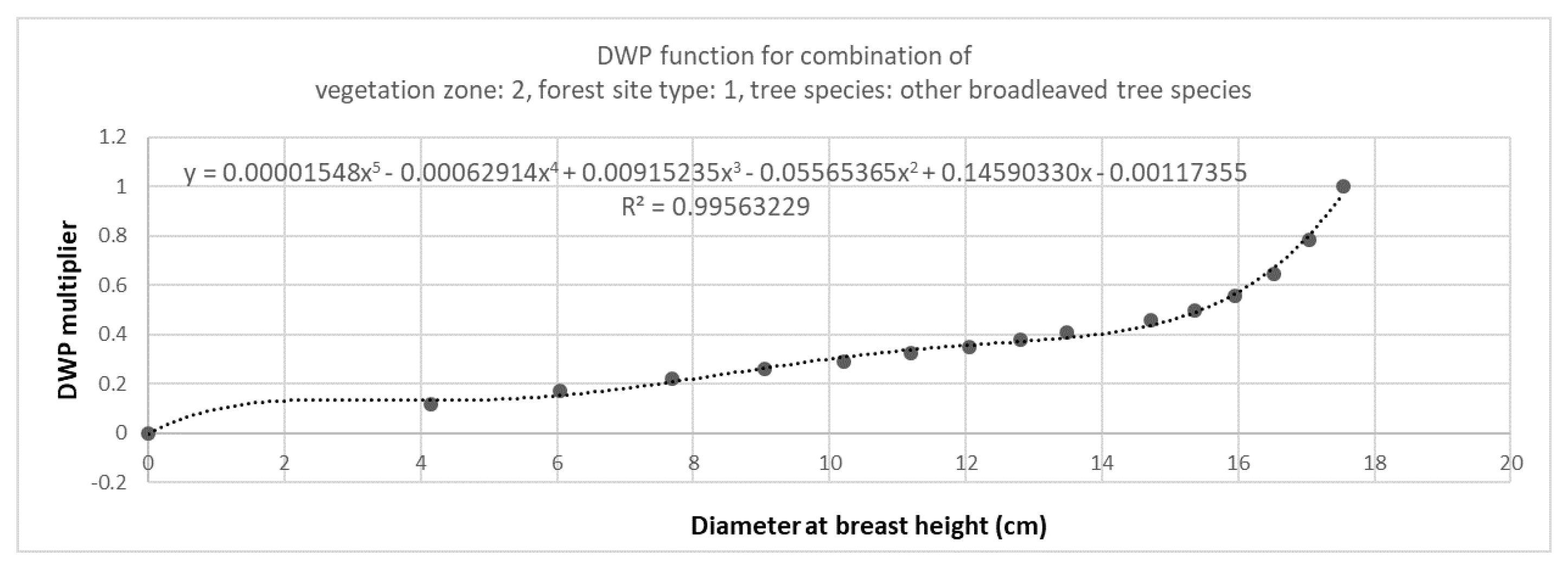
Dead Wood Potential (DWP) Functions
| Tree Species | Vegetation Zone | Forest Site Type | Functions for Dead Wood Potential (DWP) Calculation | DBH (cm) | |
| 1 | Picea abies ((L.) H. Karst.) | 1 | Herb-rich forest | y = 0.0000000161x5 − 0.0000017284x4 + 0.0000659861x3 − 0.0010311017x2 + 0.0147885592x − 0.0049002034 | 55.4 |
| 2 | Picea abies | 1 | Herb-rich heath forest | y = 0.0000000184x5 − 0.0000017033x4 + 0.0000563171x3 − 0.0007552955x2 + 0.0134742452x − 0.0023702218 | 50.7 |
| 3 | Picea abies | 1 | Mesic heath forest | y = 0.0000005264x4 − 0.0000425948x3 + 0.0011372754x2 − 0.0002934437x + 0.0169174344 | 52.6 |
| 4 | Picea abies | 1 | Sub-xeric heath forest | y = 0.0000005986x4 − 0.0000192421x3 + 0.0003016817x2 + 0.0115485958x + 0.0025994013 | 37 |
| 5 | Picea abies | 1 | Xeric heath forest | y = 0.0000002716x5 − 0.0000157163x4 + 0.0003436485x3 − 0.0030953347x2 + 0.0272649678x − 0.0038273867 | 28.8 |
| 6 | Picea abies | 1 | Barren heath forest | y = 0.0010125092x2 + 0.0150097643x + 0.0023813648 | 25 |
| 7 | Picea abies | 2 | Herb-rich forest | y = 0.0000006155x4 − 0.0000450509x3 + 0.0010562901x2 + 0.0018961460x + 0.0096330860 | 53.5 |
| 8 | Picea abies | 2 | Herb-rich heath forest | y = 0.0000006155x4 − 0.0000450509x3 + 0.0010562901x2 + 0.0018961460x + 0.0096330860 | 50.7 |
| 9 | Picea abies | 2 | Mesic heath forest | y = 0.0000005306x4 − 0.0000448023x3 + 0.0012362144x2 − 0.0014654573x + 0.0164931209 | 53.7 |
| 10 | Picea abies | 2 | Sub-xeric heath forest | y = 0.0000013384x4 − 0.0000816544x3 + 0.0017079190x2 + 0.0008330889x + 0.0132025288 | 40 |
| 11 | Picea abies | 2 | Xeric heath forest | y = 0.0000040479x4 − 0.0001761466x3 + 0.0027120941x2 + 0.0028549025x + 0.0111397051 | 29.3 |
| 12 | Picea abies | 2 | Barren heath forest | y = 0.0000092054x4 − 0.0003755234x3 + 0.0052546605x2 − 0.0051711784x + 0.0160875537 | 25.5 |
| 13 | Picea abies | 3 | Herb-rich forest | y = 0.0000122709x3 − 0.0007624465x2 + 0.0290175225x − 0.0309302578 | 48.3 |
| 14 | Picea abies | 3 | Herb-rich heath forest | y = 0.0000000372x5 − 0.0000032919x4 + 0.0001048535x3 − 0.0013661297x2 + 0.0173523584x − 0.0041851545 | 45.6 |
| 15 | Picea abies | 3 | Mesic heath forest | y = 0.0000008241x4 − 0.0000591222x3 + 0.0014262304x2 − 0.0001559167x + 0.0149484085 | 46.2 |
| 16 | Picea abies | 3 | Sub-xeric heath forest | y = 0.0000018927x4 − 0.0000772079x3 + 0.0012286067x2 + 0.0087162361x + 0.0067653140 | 31.8 |
| 17 | Picea abies | 3 | Xeric heath forest | y = 0.0000007434x5 − 0.0000389231x4 + 0.0007562472x3 − 0.0060387418x2 + 0.0369600166x − 0.0055048664 | 24.8 |
| 18 | Picea abies | 3 | Barren heath forest | y = 0.0000018814x5 − 0.0000895617x4 + 0.0015570974x3 − 0.0110989030x2 + 0.0500584897x − 0.0068869694 | 21.8 |
| 19 | Picea abies | 4 | Herb-rich forest | y = 0.0000001362x5 − 0.0000089326x4 + 0.0002173264x3 − 0.0021928022x2 + 0.0227845402x − 0.0043775857 | 33.7 |
| 20 | Picea abies | 4 | Herb-rich heath forest | y = 0.0000049058x4 − 0.0002520313x3 + 0.0043429636x2 − 0.0095134968x + 0.0253623319 | 31.3 |
| 21 | Picea abies | 4 | Mesic heath forest | y = 0.0000038422x4 − 0.0001752678x3 + 0.0028749856x2 + 0.0007796390x + 0.0148666980 | 29.8 |
| 22 | Picea abies | 4 | Sub-xeric heath forest | y = 0.0000015843x5 − 0.0000734457x4 + 0.0012755734x3 − 0.0091984010x2 + 0.0464506582x − 0.0076350317 | 21.4 |
| 23 | Picea abies | 4 | Xeric heath forest | y = 0.0000050816x5 − 0.0001963719x4 + 0.0028507686x3 − 0.0173939950x2 + 0.0655229900x − 0.0088755793 | 17.4 |
| 24 | Picea abies | 4 | Barren heath forest | y = 0.0000000094x5 − 0.0000016212x4 + 0.0001104195x3 − 0.0035850719x2 + 0.0628358948x − 0.0934533866 | 15.6 |
| 25 | Pinus sylvestris (L.) | 1 | Herb-rich forest | y = 0.0000004623x4 − 0.0000222413x3 + 0.0001927273x2 + 0.0120210416x − 0.0075600744 | 48.3 |
| 26 | Pinus sylvestris | 1 | Herb-rich heath forest | y = 0.0000000098x5 + 0.0000001796x4 − 0.0000515518x3 + 0.0015055128x2 − 0.0006701712x + 0.0042664418 | 46.7 |
| 27 | Pinus sylvestris | 1 | Mesic heath forest | y = 0.0000013512x4 − 0.0001013567x3 + 0.0023850056x2 − 0.0060850485x + 0.0064301561 | 46.7 |
| 28 | Pinus sylvestris | 1 | Sub-xeric heath forest | y = 0.0000012252x4 − 0.0000893534x3 + 0.0021243604x2 − 0.0042316368x + 0.0101178798 | 45.1 |
| 29 | Pinus sylvestris | 1 | Xeric heath forest | y = 0.0000012644x4 − 0.0000693070x3 + 0.0010995711x2 + 0.0077363288x − 0.0045700136 | 41.8 |
| 30 | Pinus sylvestris | 1 | Barren heath forest | y = 0.0000000283x5 + 0.0000006755x4 − 0.0001089991x3 + 0.0024651722x2 − 0.0018870714x + 0.0052463026 | 37.1 |
| 31 | Pinus sylvestris | 2 | Herb-rich forest | y = 0.0000009335x4 − 0.0000663941x3 + 0.0014401761x2 + 0.0015466061x + 0.0000349890 | 48.3 |
| 32 | Pinus sylvestris | 2 | Herb-rich heath forest | y = 0.0000006174x4 − 0.0000326284x3 + 0.0004487432x2 + 0.0105988127x − 0.0075041933 | 46.2 |
| 33 | Pinus sylvestris | 2 | Mesic heath forest | y = 0.0000229170x3 − 0.0010204842x2 + 0.0216302498x − 0.0105496624 | 45.7 |
| 34 | Pinus sylvestris | 2 | Sub-xeric heath forest | y = 0.0000010166x4 − 0.0000676667x3 + 0.0014820782x2 + 0.0015167476x + 0.0046006516 | 44.3 |
| 35 | Pinus sylvestris | 2 | Xeric heath forest | y = 0.0000020094x4 − 0.0001301944x3 + 0.0026234281x2 − 0.0040767151x + 0.0070796259 | 41.7 |
| 36 | Pinus sylvestris | 2 | Barren heath forest | y = 0.0000030626x4 − 0.0001696886x3 + 0.0029412809x2 − 0.0017420282x + 0.0028058062 | 36.5 |
| 37 | Pinus sylvestris | 3 | Herb-rich forest | y = 0.0000003836x4 − 0.0000136713x3 − 0.0000543905x2 + 0.0147055443x − 0.0115382974 | 47.2 |
| 38 | Pinus sylvestris | 3 | Herb-rich heath forest | y = 0.0000000581x5 − 0.0000047820x4 + 0.0001280600x3 − 0.0011291177x2 + 0.0132446600x + 0.0021001166 | 44.6 |
| 39 | Pinus sylvestris | 3 | Mesic heath forest | y = 0.0000005446x4 − 0.0000164774x3 − 0.0001563580x2 + 0.0170326122x − 0.0151731205 | 43.7 |
| 40 | Pinus sylvestris | 3 | Sub-xeric heath forest | y = 0.0000012675x4 − 0.0000882199x3 + 0.0020954396x2 − 0.0031922096x + 0.0113978403 | 42.2 |
| 41 | Pinus sylvestris | 3 | Xeric heath forest | y = 0.0000000485x5 − 0.0000019886x4 − 0.0000093689x3 + 0.0010724885x2 + 0.0036876387x + 0.0065684616 | 39.3 |
| 42 | Pinus sylvestris | 3 | Barren heath forest | y = 0.0000003745x5 − 0.0000274009x4 + 0.0007016601x3 − 0.0072645366x2 + 0.0404266958x − 0.0025942599 | 34.5 |
| 43 | Pinus sylvestris | 4 | Herb-rich forest | y = 0.0000201272x3 − 0.0007666773x2 + 0.0187609364x − 0.0056661884 | 43.7 |
| 44 | Pinus sylvestris | 4 | Herb-rich heath forest | y = 0.0000225723x3 − 0.0006202513x2 + 0.0177580701x − 0.0011832482 | 38.1 |
| 45 | Pinus sylvestris | 4 | Mesic heath forest | y = 0.0000127058x3 + 0.0001898738x2 + 0.0042006395x + 0.0443521300 | 36 |
| 46 | Pinus sylvestris | 4 | Sub-xeric heath forest | y = 0.0000116647x3 + 0.0000042624x2 + 0.0117378253x + 0.0070122178 | 36.3 |
| 47 | Pinus sylvestris | 4 | Xeric heath forest | y = 0.0000038240x4 − 0.0001528377x3 + 0.0019583311x2 + 0.0093019582x − 0.0011384075 | 30.2 |
| 48 | Pinus sylvestris | 4 | Barren heath forest | y = 0.0000759311x3 − 0.0018448651x2 + 0.0292579425x − 0.0051270841 | 27.8 |
| 49 | Betula pendula (Roth) | 1 | Herb-rich forest | y = 0.0000000698x5 − 0.0000029907x4 + 0.0000126208x3 + 0.0006443447x2 + 0.0081154853x + 0.0028446742 | 36.8 |
| 50 | Betula pendula | 1 | Herb-rich heath forest | y = 0.0000004286x5 − 0.0000315153x4 + 0.0008107264x3 − 0.0084532404x2 + 0.0439597902x − 0.0043918714 | 34.5 |
| 51 | Betula pendula | 1 | Mesic heath forest | y = 0.0000004916x5 − 0.0000342620x4 + 0.0008300406x3 − 0.0080614969x2 + 0.0409280753x − 0.0062904828 | 33.1 |
| 52 | Betula pendula | 1 | Sub-xeric heath forest | y = 0.0000848874x3 − 0.0025538279x2 + 0.0357856249x − 0.0197727664 | 29.7 |
| 53 | Betula pendula | 1 | Xeric heath forest | y = 0.0000026167x5 − 0.0000929878x4 + 0.0011342487x3 − 0.0054258503x2 + 0.0332693801x + 0.0003155131 | 19.8 |
| 54 | Betula pendula | 1 | Barren heath forest | y = 0.0000124704x5 − 0.0004611922x4 + 0.0060537298x3 − 0.0328496818x2 + 0.0907612742x − 0.0041143955 | 17 |
| 55 | Betula pendula | 2 | Herb-rich forest | y = 0.0000023886x4 − 0.0001199093x3 + 0.0017604835x2 + 0.0064533491x + 0.0003928322 | 36.8 |
| 56 | Betula pendula | 2 | Herb-rich heath forest | y = 0.0000001835x5 − 0.0000111267x4 + 0.0002244220x3 − 0.0016810971x2 + 0.0179017119x + 0.0010852197 | 34.4 |
| 57 | Betula pendula | 2 | Mesic heath forest | y = 0.0000006281x5 − 0.0000454954x4 + 0.0011532698x3 − 0.0118540667x2 + 0.0561558320x − 0.0080901647 | 33 |
| 58 | Betula pendula | 2 | Sub-xeric heath forest | y = 0.0000800245x3 − 0.0022774568x2 + 0.0326993896x − 0.0144578193 | 29.5 |
| 59 | Betula pendula | 2 | Xeric heath forest | y = 0.0000041677x5 − 0.0001574013x4 + 0.0020859079x3 − 0.0112566189x2 + 0.0463268449x − 0.0010374605 | 19.3 |
| 60 | Betula pendula | 2 | Barren heath forest | y = 0.0000129718x5 − 0.0004756278x4 + 0.0061959914x3 − 0.0334149409x2 + 0.0918745245x − 0.0041449752 | 16.8 |
| 61 | Betula pendula | 3 | Herb-rich forest | y = 0.0000000812x5 − 0.0000025757x4 − 0.0000173798x3 + 0.0010223015x2 + 0.0081035278x + 0.0043284919 | 34.1 |
| 62 | Betula pendula | 3 | Herb-rich heath forest | y = 0.0000007434x5 − 0.0000509956x4 + 0.0012244189x3 − 0.0119180632x2 + 0.0550499985x − 0.0089540976 | 31.4 |
| 63 | Betula pendula | 3 | Mesic heath forest | y = 0.0000044906x4 − 0.0001489538x3 + 0.0013133137x2 + 0.0156569208x − 0.0038277485 | 28.6 |
| 64 | Betula pendula | 3 | Sub-xeric heath forest | y = 0.0000843469x3 − 0.0014555367x2 + 0.0237551975x + 0.0050821260 | 25.2 |
| 65 | Betula pendula | 3 | Xeric heath forest | y = 0.0000134762x5 − 0.0004836110x4 + 0.0061431121x3 − 0.0320798098x2 + 0.0873219905x − 0.0061012210 | 16.6 |
| 66 | Betula pendula | 3 | Barren heath forest | y = 0.0000276450x5 − 0.0008898351x4 + 0.0101340238x3 − 0.0473476725x2 + 0.1086884842x − 0.0051200733 | 14.7 |
| 67 | Betula pendula | 4 | Herb-rich forest | y = 0.0000142294x3 + 0.0006851383x2 + 0.0038379153x + 0.0305639777 | 28.5 |
| 68 | Betula pendula | 4 | Herb-rich heath forest | y = 0.0000821947x3 − 0.0013489222x2 + 0.0225653406x + 0.0086468736 | 25.2 |
| 69 | Betula pendula | 4 | Mesic heath forest | y = 0.0001487373x3 − 0.0032477261x2 + 0.0384672973x − 0.0112808847 | 23.5 |
| 70 | Betula pendula | 4 | Sub-xeric heath forest | y = 0.0000237811x4 − 0.0006969965x3 + 0.0063541234x2 + 0.0058201682x + 0.0066524128 | 20.7 |
| 71 | Betula pendula | 4 | Xeric heath forest | y = 0.0000341585x5 − 0.0010567167x4 + 0.0115821628x3 − 0.0522670867x2 + 0.1164330642x − 0.0110599387 | 14.1 |
| 72 | Betula pendula | 4 | Barren heath forest | y = 0.0000607977x5 − 0.0017280977x4 + 0.0173812267x3 − 0.0718177791x2 + 0.1399870537x − 0.0109816278 | 12.8 |
| 73 | Betula pubescens (Ehrh.) | 1 | Herb-rich forest | y = 0.0000005147x5 − 0.0000397530x4 + 0.0010706348x3 − 0.0116114394x2 + 0.0563842058x − 0.0081785677 | 34.6 |
| 74 | Betula pubescens | 1 | Herb-rich heath forest | y = 0.0000008478x5 − 0.0000578998x4 + 0.0013844346x3 − 0.0134123160x2 + 0.0598250568x − 0.0064807858 | 30.8 |
| 75 | Betula pubescens | 1 | Mesic heath forest | y = 0.0000008494x5 − 0.0000570531x4 + 0.0013427466x3 − 0.0128234040x2 + 0.0577501024x − 0.0077276424 | 30.4 |
| 76 | Betula pubescens | 1 | Sub-xeric heath forest | y = 0.0000011998x5 − 0.0000697299x4 + 0.0014158143x3 − 0.0115995601x2 + 0.0505531563x − 0.0090827056 | 27.2 |
| 77 | Betula pubescens | 1 | Xeric heath forest | y = 0.0000195064x5 − 0.0006349216x4 + 0.0073406555x3 − 0.0351181493x2 + 0.0908986831x − 0.0032060826 | 15.2 |
| 78 | Betula pubescens | 1 | Barren heath forest | y = 0.0000016683x5 − 0.0000969083x4 + 0.0021895457x3 − 0.0235631730x2 + 0.1367625836x − 0.1076733924 | 13.2 |
| 79 | Betula pubescens | 2 | Herb-rich forest | y = 0.0000005078x5 − 0.0000396260x4 + 0.0010777939x3 − 0.0118120982x2 + 0.0575682212x − 0.0096812959 | 34.9 |
| 80 | Betula pubescens | 2 | Herb-rich heath forest | y = 0.0000007892x5 − 0.0000545302x4 + 0.0013190001x3 − 0.0129279489x2 + 0.0586627985x − 0.0068225071 | 31.1 |
| 81 | Betula pubescens | 2 | Mesic heath forest | y = 0.0000009307x5 − 0.0000626945x4 + 0.0014860637x3 − 0.0143806824x2 + 0.0637802760x − 0.0046716255 | 30.1 |
| 82 | Betula pubescens | 2 | Sub-xeric heath forest | y = 0.0000013047x5 − 0.0000748816x4 + 0.0015031182x3 − 0.0121962798x2 + 0.0522196363x − 0.0092041945 | 26.8 |
| 83 | Betula pubescens | 2 | Xeric heath forest | y = 0.0000199097x5 − 0.0006442758x4 + 0.0074117015x3 − 0.0353237563x2 + 0.0913360115x − 0.0032317430 | 15.1 |
| 84 | Betula pubescens | 2 | Barren heath forest | y = 0.0000434301x5 − 0.0012348638x4 + 0.0125008008x3 − 0.0525099819x2 + 0.1142383729x − 0.0022700043 | 13.1 |
| 85 | Betula pubescens | 3 | Herb-rich forest | y = 0.0000008926x5 − 0.0000586134x4 + 0.0013438732x3 − 0.0124500644x2 + 0.0553706773x − 0.0088025839 | 30.1 |
| 86 | Betula pubescens | 3 | Herb-rich heath forest | y = 0.0000011983x5 − 0.0000734126x4 + 0.0015788582x3 − 0.0138170861x2 + 0.0589918348x − 0.0079444343 | 27.9 |
| 87 | Betula pubescens | 3 | Mesic heath forest | y = 0.0000024729x5 − 0.0001290246x4 + 0.0023699864x3 − 0.0177546791x2 + 0.0658269113x − 0.0055008469 | 23.9 |
| 88 | Betula pubescens | 3 | Sub-xeric heath forest | y = 0.0003131284x3 − 0.0068869653x2 + 0.0632760365x − 0.0340467609 | 20 |
| 89 | Betula pubescens | 3 | Xeric heath forest | y = 0.0000469941x5 − 0.0013264440x4 + 0.0132503785x3 − 0.0542358803x2 + 0.1129146343x − 0.0040491170 | 13 |
| 90 | Betula pubescens | 3 | Barren heath forest | y = 0.0000973178x5 − 0.0024765182x4 + 0.0223414139x3 − 0.0827234057x2 + 0.1457634078x − 0.0033752688 | 11.5 |
| 91 | Betula pubescens | 4 | Herb-rich forest | y = 0.0001056533x3 − 0.0018595467x2 + 0.0276357197x + 0.0014319387 | 23.7 |
| 92 | Betula pubescens | 4 | Herb-rich heath forest | y = 0.0000135491x4 − 0.0002887099x3 + 0.0014516350x2 + 0.0247671329x − 0.0038273969 | 20.5 |
| 93 | Betula pubescens | 4 | Mesic heath forest | y = 0.0000520241x4 − 0.0015190382x3 + 0.0140511857x2 − 0.0150064164x + 0.0165457552 | 18.4 |
| 94 | Betula pubescens | 4 | Sub-xeric heath forest | y = 0.0000946763x4 − 0.0025073073x3 + 0.0211413109x2 − 0.0274326999x + 0.0237633916 | 16.1 |
| 95 | Betula pubescens | 4 | Xeric heath forest | y = 0.0001112251x5 − 0.0027012577x4 + 0.0231219019x3 − 0.0808900733x2 + 0.1407658016x − 0.0085794462 | 11.1 |
| 96 | Betula pubescens | 4 | Barren heath forest | y = 0.0002010279x5 − 0.0045434558x4 + 0.0360747028x3 − 0.1164661501x2 + 0.1750207637x − 0.0087745744 | 10.2 |
| 97 | Populus tremula (L.) | 1 | Herb-rich forest | y = 0.0000004911x5 − 0.0000364224x4 + 0.0009463543x3 − 0.0099537068x2 + 0.0497723271x − 0.0052573545 | 33.7 |
| 98 | Populus tremula | 1 | Herb-rich heath forest | y = 0.0000006389x5 − 0.0000448857x4 + 0.0011066815x3 − 0.0110807294x2 + 0.0529277624x − 0.0053017914 | 31.9 |
| 99 | Populus tremula | 1 | Mesic heath forest | y = 0.0000079795x4 − 0.0004296518x3 + 0.0072278336x2 − 0.0222549155x + 0.0216449596 | 31.4 |
| 100 | Populus tremula | 1 | Sub-xeric heath forest | y = 0.0000025340x5 − 0.0001252167x4 + 0.0021839468x3 − 0.0155782893x2 + 0.0596280231x − 0.0065490851 | 23 |
| 101 | Populus tremula | 1 | Xeric heath forest | y = 0.0000113631x5 − 0.0004077298x4 + 0.0051975367x3 − 0.0273533659x2 + 0.0790810564x − 0.0031555977 | 16.8 |
| 102 | Populus tremula | 1 | Barren heath forest | y = 0.0000233258x5 − 0.0007620291x4 + 0.0088408222x3 − 0.0423768934x2 + 0.1028515013x − 0.0028496552 | 15 |
| 103 | Populus tremula | 2 | Herb-rich forest | y = 0.0000004952x5 − 0.0000373045x4 + 0.0009829351x3 − 0.0104664729x2 + 0.0520280776x − 0.0067635479 | 34 |
| 104 | Populus tremula | 2 | Herb-rich heath forest | y = 0.0000005734x5 − 0.0000429847x4 + 0.0011286691x3 − 0.0120179552x2 + 0.0581328449x − 0.0081317520 | 33.5 |
| 105 | Populus tremula | 2 | Mesic heath forest | y = 0.0000084733x4 − 0.0004459214x3 + 0.0073424690x2 − 0.0218166161x + 0.0214580688 | 30.8 |
| 106 | Populus tremula | 2 | Sub-xeric heath forest | y = 0.0000026447x5 − 0.0001281296x4 + 0.0021927625x3 − 0.0153685162x2 + 0.0588012658x − 0.0058806919 | 22.7 |
| 107 | Populus tremula | 2 | Xeric heath forest | y = 0.0000108433x5 − 0.0003926531x4 + 0.0050555795x3 − 0.0269215264x2 + 0.0788169919x − 0.0034048924 | 17 |
| 108 | Populus tremula | 2 | Barren heath forest | y = 0.0000245697x5 − 0.0007935809x4 + 0.0091121621x3 − 0.0432970898x2 + 0.1043628446x − 0.0028581742 | 14.8 |
| 109 | Populus tremula | 3 | Herb-rich forest | y = 0.0000005817x5 − 0.0000388786x4 + 0.0009104427x3 − 0.0086232657x2 + 0.0433743113x − 0.0060358705 | 31.2 |
| 110 | Populus tremula | 3 | Herb-rich heath forest | y = 0.0000008455x5 − 0.0000541241x4 + 0.0012171283x3 − 0.0111218403x2 + 0.0512982223x − 0.0068051191 | 29.4 |
| 111 | Populus tremula | 3 | Mesic heath forest | y = 0.0001562745x3 − 0.0046067531x2 + 0.0537072162x − 0.0412866515 | 26 |
| 112 | Populus tremula | 3 | Sub-xeric heath forest | y = 0.0003543187x3 − 0.0078771000x2 + 0.0700779711x − 0.0376300965 | 19.6 |
| 113 | Populus tremula | 3 | Xeric heath forest | y = 0.0000206683x5 − 0.0006761866x4 + 0.0078290083x3 − 0.0371976946x2 + 0.0928146663x − 0.0049042456 | 15.2 |
| 114 | Populus tremula | 3 | Barren heath forest | y = 0.0000439513x5 − 0.0012918402x4 + 0.0134394830x3 − 0.0573061683x2 + 0.1192271055x − 0.0040964012 | 13.4 |
| 115 | Populus tremula | 4 | Herb-rich forest | y = 0.0000048016x4 − 0.0001117991x3 + 0.0003543209x2 + 0.0226836786x − 0.0063111968 | 25.8 |
| 116 | Populus tremula | 4 | Herb-rich heath forest | y = 0.0000919159x3 − 0.0013406533x2 + 0.0229964151x + 0.0086222734 | 23.7 |
| 117 | Populus tremula | 4 | Mesic heath forest | y = 0.0001862663x3 − 0.0038237204x2 + 0.0422245854x − 0.0127054555 | 21.8 |
| 118 | Populus tremula | 4 | Sub-xeric heath forest | y = 0.0000116611x5 − 0.0003967235x4 + 0.0047990655x3 − 0.0240006334x2 + 0.0726713154x − 0.0077883137 | 16.3 |
| 119 | Populus tremula | 4 | Xeric heath forest | y = 0.0000449284x5 − 0.0013038827x4 + 0.0133998791x3 − 0.0566353526x2 + 0.1195635316x − 0.0100572770 | 13.3 |
| 120 | Populus tremula | 4 | Barren heath forest | y = 0.0000843400x5 − 0.0022248614x4 + 0.0207460282x3 − 0.0793170088x2 + 0.1446013272x − 0.0096399207 | 11.9 |
| 121 | Alnus glutinosa ((L.) Gaertn.) | 1 | Herb-rich forest | y = 0.0000074496x5 − 0.0003525090x4 + 0.0059404760x3 − 0.0415701978x2 + 0.1244785725x − 0.0023168716 | 20.5 |
| 122 | Alnus glutinosa | 1 | Herb-rich heath forest | y = 0.0000128704x5 − 0.0005507459x4 + 0.0084512065x3 − 0.0543659749x2 + 0.1493117306x − 0.0015781598 | 18.3 |
| 123 | Alnus glutinosa | 1 | Mesic heath forest | y = 0.0000120440x5 − 0.0004985693x4 + 0.0073668242x3 − 0.0453107979x2 + 0.1239013027x − 0.0021327974 | 18.1 |
| 124 | Alnus glutinosa | 1 | Sub-xeric heath forest | y = 0.0000988573x5 − 0.0026154349x4 + 0.0245845858x3 − 0.0956244366x2 + 0.1696714860x − 0.0020026933 | 11.8 |
| 125 | Alnus glutinosa | 1 | Xeric heath forest | y = 0.0004043769x5 − 0.0089613217x4 + 0.0712133327x3 − 0.2367022954x2 + 0.3241998142x − 0.0006634528 | 9.37 |
| 126 | Alnus glutinosa | 1 | Barren heath forest | y = 0.0053924930x3 − 0.0590984236x2 + 0.2201961376x − 0.0256368371 | 8.4 |
| 127 | Alnus glutinosa | 2 | Herb-rich forest | y = 0.0000075081x5 − 0.0003506327x4 + 0.0058294432x3 − 0.0402069148x2 + 0.1199446382x − 0.0026136340 | 20.3 |
| 128 | Alnus glutinosa | 2 | Herb-rich heath forest | y = 0.0000145047x5 − 0.0006014285x4 + 0.0089383388x3 − 0.0556707462x2 + 0.1490098749x − 0.0016618983 | 17.8 |
| 129 | Alnus glutinosa | 2 | Mesic heath forest | y = 0.0000132149x5 − 0.0005805631x4 + 0.0091730318x3 − 0.0610986544x2 + 0.1701848768x − 0.0011818426 | 18.5 |
| 130 | Alnus glutinosa | 2 | Sub-xeric heath forest | y = 0.0019794703x3 − 0.0307260916x2 + 0.1574728842x − 0.0118975512 | 12 |
| 131 | Alnus glutinosa | 2 | Xeric heath forest | y = 0.0004318896x5 − 0.0094351732x4 + 0.0739824124x3 − 0.2429702683x2 + 0.3295543992x − 0.0006597002 | 9.23 |
| 132 | Alnus glutinosa | 2 | Barren heath forest | y = 0.0057173199x3 − 0.0617247899x2 + 0.2259910364x − 0.0255182941 | 8.26 |
| 133 | Alnus glutinosa | 3 | Herb-rich forest | y = 0.0000082551x5 − 0.0003559860x4 + 0.0054499415x3 − 0.0344546810x2 + 0.1004627207x − 0.0032690688 | 19.2 |
| 134 | Alnus glutinosa | 3 | Herb-rich heath forest | y = 0.0000141998x5 − 0.0005663320x4 + 0.0080472709x3 − 0.0475170982x2 + 0.1254229615x − 0.0030199959 | 17.5 |
| 135 | Alnus glutinosa | 3 | Mesic heath forest | y = 0.0000162769x5 − 0.0005859380x4 + 0.0075014554x3 − 0.0397237899x2 + 0.1025931440x − 0.0025992132 | 16.3 |
| 136 | Alnus glutinosa | 3 | Sub-xeric heath forest | y = 0.0001040101x5 − 0.0027123121x4 + 0.0250222206x3 − 0.0946173574x2 + 0.1625612077x − 0.0038541966 | 11.6 |
| 137 | Alnus glutinosa | 3 | Xeric heath forest | y = 0.0003465269x5 − 0.0075489957x4 + 0.0583114029x3 − 0.1852030100x2 + 0.2496181502x − 0.0024301401 | 9.47 |
| 138 | Alnus glutinosa | 3 | Barren heath forest | y = 0.0006307148x5 − 0.0127831695x4 + 0.0918602416x3 − 0.2716487035x2 + 0.3275330978x − 0.0017410250 | 8.66 |
| 139 | Alnus glutinosa | 4 | Herb-rich forest | y = 0.0000109015x5 − 0.0004002291x4 + 0.0052118785x3 − 0.0279047711x2 + 0.0799147601x − 0.0042342366 | 17.1 |
| 140 | Alnus glutinosa | 4 | Herb-rich heath forest | y = 0.0000232563x5 − 0.0007786065x4 + 0.0092497879x3 − 0.0451945856x2 + 0.1074552414x − 0.0040762029 | 15.2 |
| 141 | Alnus glutinosa | 4 | Mesic heath forest | y = 0.0000222440x5 − 0.0007248221x4 + 0.0083510986x3 − 0.0394504590x2 + 0.0966699136x − 0.0079985370 | 15 |
| 142 | Alnus glutinosa | 4 | Sub-xeric heath forest | y = 0.0001195714x5 − 0.0029180046x4 + 0.0250762833x3 − 0.0880100258x2 + 0.1496041466x − 0.0094044374 | 11.1 |
| 143 | Alnus glutinosa | 4 | Xeric heath forest | y = 0.0003526446x5 − 0.0074890484x4 + 0.0557315217x3 − 0.1679583885x2 + 0.2211855538x − 0.0091879247 | 9.41 |
| 144 | Alnus glutinosa | 4 | Barren heath forest | y = 0.0049165839x3 − 0.0569047042x2 + 0.2187235843x − 0.0565417242 | 8.77 |
| 145 | Other broadleaved | 1 | Herb-rich forest | y = 0.0000159331x5 − 0.0006551323x4 + 0.0096463222x3 − 0.0594495816x2 + 0.1557082599x − 0.0009990372 | 17.6 |
| 146 | Other broadleaved | 1 | Herb-rich heath forest | y = 0.0000205100x5 − 0.0007254342x4 + 0.0093421540x3 − 0.0512173513x2 + 0.1319081391x − 0.0004774367 | 15.4 |
| 147 | Other broadleaved | 1 | Mesic heath forest | y = 0.0000401044x5 − 0.0013620237x4 + 0.0166251208x3 − 0.0854673359x2 + 0.1885573057x − 0.0007201616 | 14.6 |
| 148 | Other broadleaved | 1 | Sub-xeric heath forest | y = 0.0002650248x5 − 0.0060471431x4 + 0.0492898767x3 − 0.1672909525x2 + 0.2451454027x − 0.0006349294 | 9.91 |
| 149 | Other broadleaved | 1 | Xeric heath forest | y = 0.0026390485x4 − 0.0378261877x3 + 0.1704826425x2 − 0.1726942108x + 0.0023550176 | 7.95 |
| 150 | Other broadleaved | 1 | Barren heath forest | y = 0.0093497583x3 − 0.0837830610x2 + 0.2517833753x − 0.0135120058 | 7.01 |
| 151 | Other broadleaved | 2 | Herb-rich forest | y = 0.0000154781x5 − 0.0006291426x4 + 0.0091523543x3 − 0.0556536543x2 + 0.1459033017x − 0.0011735548 | 17.5 |
| 152 | Other broadleaved | 2 | Herb-rich heath forest | y = 0.0010104419x3 − 0.0177529097x2 + 0.1097035692x − 0.0173601891 | 14.3 |
| 153 | Other broadleaved | 2 | Mesic heath forest | y = 0.0009902020x3 − 0.0180949531x2 + 0.1133238427x − 0.0136136818 | 14.7 |
| 154 | Other broadleaved | 2 | Sub-xeric heath forest | y = 0.0002614646x5 − 0.0059727446x4 + 0.0487995206x3 − 0.1663751121x2 + 0.2456566987x − 0.0006193862 | 9.92 |
| 155 | Other broadleaved | 2 | Xeric heath forest | y = 0.0070031761x3 − 0.0686189565x2 + 0.2293861734x − 0.0180324391 | 7.67 |
| 156 | Other broadleaved | 2 | Barren heath forest | y = 0.0096623996x3 − 0.0864707998x2 + 0.2587742488x − 0.0141651976 | 6.95 |
| 157 | Other broadleaved | 3 | Herb-rich forest | y = 0.0000191741x5 − 0.0007210959x4 + 0.0096521416x3 − 0.0536080315x2 + 0.1325356110x − 0.0018781810 | 16.5 |
| 158 | Other broadleaved | 3 | Herb-rich heath forest | y = 0.0000341563x5 − 0.0011529939x4 + 0.0139572824x3 − 0.0707435928x2 + 0.1588258703x − 0.0012299346 | 14.7 |
| 159 | Other broadleaved | 3 | Mesic heath forest | y = 0.0000440456x5 − 0.0013787066x4 + 0.0153463234x3 − 0.0707112495x2 + 0.1470997311x − 0.0013175106 | 13.9 |
| 160 | Other broadleaved | 3 | Sub-xeric heath forest | y = 0.0002722786x5 − 0.0060045435x4 + 0.0469498663x3 − 0.1510238501x2 + 0.2142271115x − 0.0017976770 | 9.74 |
| 161 | Other broadleaved | 3 | Xeric heath forest | y = 0.0009667794x5 − 0.0183945971x4 + 0.1240917529x3 − 0.3448562969x2 + 0.3852069122x − 0.0009318150 | 8.09 |
| 162 | Other broadleaved | 3 | Barren heath forest | y = 0.0076237774x3 − 0.0730281879x2 + 0.2298242375x − 0.0247438319 | 7.54 |
| 163 | Other broadleaved | 4 | Herb-rich forest | y = 0.0000323070x5 − 0.0010219432x4 + 0.0114310178x3 − 0.0524164810x2 + 0.1155566015x − 0.0031287472 | 14.4 |
| 164 | Other broadleaved | 4 | Herb-rich heath forest | y = 0.0000634743x5 − 0.0018274664x4 + 0.0186526646x3 − 0.0783238736x2 + 0.1495900203x − 0.0025211789 | 12.8 |
| 165 | Other broadleaved | 4 | Mesic heath forest | y = 0.0000571733x5 − 0.0015683402x4 + 0.0151450449x3 − 0.0595812600x2 + 0.1177980604x − 0.0055481454 | 12.7 |
| 166 | Other broadleaved | 4 | Sub-xeric heath forest | y = 0.0003133823x5 − 0.0064099859x4 + 0.0458978425x3 − 0.1330159652x2 + 0.1814353937x − 0.0061431270 | 9.31 |
| 167 | Other broadleaved | 4 | Xeric heath forest | y = 0.0007835618x5 − 0.0145607268x4 + 0.0942725426x3 − 0.2456538957x2 + 0.2703820828x − 0.0062743999 | 8.24 |
| 168 | Other broadleaved | 4 | Barren heath forest | y = 0.0011059106x5 − 0.0200709884x4 + 0.1267110787x3 − 0.3214094244x2 + 0.3292721334x − 0.0068760501 | 7.94 |
References
- Sala, O.E.; Chapin, F.S.; Armesto, J.J.; Berlow, E.; Bloomfield, J.; Dirzo, R.; Huber-Sanwald, E.; Huenneke, L.F.; Jackson, R.B.; Kinzig, A.; et al. Biodiversity—Global biodiversity scenarios for the year 2100. Science 2000, 287, 1770–1774. [Google Scholar] [CrossRef] [PubMed]
- Montanarella, L.; Scholes, R.; Brainich, A.I. The Ipbes Assessment Report on Land Degradation and Restoration; IPBES—Secretariat of the Intergovernmental Science-Policy Platform on Biodiversity and Ecosystem Services: Bonn, Germany, 2018. [Google Scholar] [CrossRef]
- Esseen, P.-A.; Ehnström, B.; Ericson, L.; Sjöberg, K. Boreal forests. Ecol. Bull. 1997, 46, 16–47. [Google Scholar]
- Hansen, A.J.; Spies, T.A.; Swanson, F.J.; Ohmann, J.L. Conserving biodiversity in managed forests. BioScience 1991, 41, 382–392. [Google Scholar] [CrossRef] [Green Version]
- Gauthier, S.; Bernier, P.; Kuuluvainen, T.; Shvidenko, A.Z.; Schepaschenko, D.G. Boreal forest health and global change. Science 2015, 349, 819–822. [Google Scholar] [CrossRef]
- Wallenius, T.; Niskanen, L.; Virtanen, T.; Hottola, J.; Brumelis, G.; Angervuori, A.; Julkunen, J.; Pihlström, M. Loss of habitats, naturalness and species diversity in Eurasian forest landscapes. Ecol. Indic. 2010, 10, 1093–1101. [Google Scholar] [CrossRef]
- Peltola, A.; Ihalainen, A.; Mäki-Simola, E.; Sauvula-Seppälä, T.; Torvelainen, J.; Uotila, E.; Vaahtera, E.; Ylitalo, E. Suomen Metsätilastot—Finnish Forest Statistics; Luke Natural Resources Institute Finland: Helsinki, Finland, 2019; p. 200. [Google Scholar]
- Kontula, T.; Raunio, A. Threatened Habitat Types in Finland 2018. Red List of Habitats—Results and Basis for Assessment; Finnish Environment Institute and Ministry of the Environment: Helsinki, Finland, 2019; Volume 2, p. 254.
- Kouki, J.; Junninen, K.; Mäkelä, K.; Hokkanen, M.; Aakala, A.; Hallikainen, V.; Korhonen, K.T.; Kuuluvainen, T.; Loiskekoski, M.; Mattila, O.; et al. Forests. In Threatened Habitat Types in Finland 2018. Red List of Habitats—Results and Basis for Assessment; Kontula, T., Raunio, A., Eds.; Finnish Environment Institute and Ministry of the Environment: Helsinki, Finland, 2018; pp. 475–567. [Google Scholar]
- Hyvärinen, E.; Juslén, A.; Kemppainen, E.; Uddström, A.; Liukko, U.-M. The 2019 Red List of Finnish Species; Ministry of the Environment & Finnish Environment Institute: Helsinki, Finland, 2019; p. 704.
- Watson, J.E.M.; Evans, T.; Venter, O.; Williams, B.; Tulloch, A.; Stewart, C.; Thompson, I.; Ray, J.C.; Murray, K.; Salazar, A.; et al. The exceptional value of intact forest ecosystems. Nat. Ecol. Evol. 2018, 2, 599–610. [Google Scholar] [CrossRef]
- Punttila, P.; Ihalainen, A. Luonnontilaisen kaltaiset metsät suojelu- ja ei-suojelluilla alueilla (Old growth forests in conservation and non-conservation areas, in Finnish). [Updated version]; In METSOn Jäljillä—Etelä-Suomen Metsien Monimuotoisuusohjelman Tutkimusraportti; Horne, P., Koskela, T., Kuusinen, M., Otsamo, A., Syrjänen, K., Eds.; Ministry of Agriculture and Forestry & Ministry of Environment & Finnish Forest Research Institute METLA & Finnish Environment Institute: Vammala, Finland, 2006; p. 19. [Google Scholar]
- Korhonen, A.; Siitonen, J.; Kotze, D.J.; Immonen, A.; Hamberg, L. Stand characteristics and dead wood in urban forests: Potential biodiversity hotspots in managed boreal landscapes. Landsc. Urban Plan. 2020, 201, 12. [Google Scholar] [CrossRef]
- Aakala, T. Coarse woody debris in late-successional Picea abies forests in northern Europe: Variability in quantities and models of decay class dynamics. For. Ecol. Manag. 2010, 260, 770–779. [Google Scholar] [CrossRef]
- Siitonen, J. Forest management, coarse woody debris and saproxylic organisms: Fennoscandian boreal forests as an example. Ecol. Bull. 2001, 49, 11–41. [Google Scholar]
- Stokland, J.N. The coarse woody debris profile: An archive of recent forest history and an important biodiversity indicator. Ecol. Bull. 2001, 49, 71–83. [Google Scholar]
- Paillet, Y.; Bergès, L.; Hjältén, J.; Ódor, P.; Avon, C.; Bernhardt--Römermann, M.; Bijlsma, R.-J.; De Bruyn, L.; Fuhr, M.; Grandin, U. Biodiversity differences between managed and unmanaged forests: Meta--Analysis of species richness in Europe. Conserv. Biol. 2010, 24, 101–112. [Google Scholar] [CrossRef] [PubMed]
- Lassauce, A.; Paillet, Y.; Jactel, H.; Bouget, C. Deadwood as a surrogate for forest biodiversity: Meta-analysis of correlations between deadwood volume and species richness of saproxylic organisms. Ecol. Indic. 2011, 11, 1027–1039. [Google Scholar] [CrossRef]
- Junninen, K.; Komonen, A. Conservation ecology of boreal polypores: A review. Biol. Conserv. 2011, 144, 11–20. [Google Scholar] [CrossRef]
- Gao, T.; Nielsen, A.B.; Hedblom, M. Reviewing the strength of evidence of biodiversity indicators for forest ecosystems in Europe. Ecol. Indic. 2015, 57, 420–434. [Google Scholar] [CrossRef]
- Tomppo, E.; Heikkinen, J.; Henttonen, H.M.; Ihalainen, A.; Katila, M.; Mäkelä, H.; Tuomainen, T.; Vainikainen, N. Designing and Conducting a Forest Inventory—Case: 9th National Forest Inventory of Finland; Springer: Berlin, Germany, 2011. [Google Scholar]
- Russell, M.B.; Fraver, S.; Aakala, T.; Gove, J.H.; Woodall, C.W.; D’Amato, A.W.; Ducey, M.J. Quantifying carbon stores and decomposition in dead wood: A review. For. Ecol. Manag. 2015, 350, 107–128. [Google Scholar] [CrossRef]
- Ranius, T.; Kindvall, O.; Kruys, N.; Jonsson, B.G. Modelling dead wood in Norway spruce stands subject to different management regimes. For. Ecol. Manag. 2003, 182, 13–29. [Google Scholar] [CrossRef]
- Kimberley, M.O.; Beets, P.N.; Paul, T.S.H. Comparison of measured and modelled change in coarse woody debris carbon stocks in New Zealand’s natural forest. For. Ecol. Manag. 2019, 434, 18–28. [Google Scholar] [CrossRef]
- Goodale, C.L.; Apps, M.J.; Birdsey, R.A.; Field, C.B.; Heath, L.S.; Houghton, R.A.; Jenkins, J.C.; Kohlmaier, G.H.; Kurz, W.; Liu, S.R.; et al. Forest carbon sinks in the Northern Hemisphere. Ecol. Appl. 2002, 12, 891–899. [Google Scholar] [CrossRef]
- Mäkinen, H.; Hynynen, J.; Siitonen, J.; Sievänen, R. Predicting the Decomposition of Scots pine, Norway spruce, and Birch Stems in Finland. Ecol. Appl. 2006, 16, 1865–1879. [Google Scholar] [CrossRef]
- Kangas, A.; Astrup, R.; Breidenbach, J.; Fridman, J.; Gobakken, T.; Korhonen, K.T.; Maltamo, M.; Nilsson, M.; Nord-Larsen, T.; Næsset, E.; et al. Remote sensing and forest inventories in Nordic countries—Roadmap for the future. Scand. J. For. Res. 2018, 33, 397–412. [Google Scholar] [CrossRef] [Green Version]
- Tanhuanpää, T.; Kankare, V.; Vastaranta, M.; Saarinen, N.; Holopainen, M. Monitoring downed coarse woody debris through appearance of canopy gaps in urban boreal forests with bitemporal ALS data. Urban For. Urban Green. 2015, 14, 835–843. [Google Scholar] [CrossRef]
- Pesonen, A.; Maltamo, M.; Eerikainen, K.; Packalen, P. Airborne laser scanning-based prediction of coarse woody debris volumes in a conservation area. For. Ecol. Manag. 2008, 255, 3288–3296. [Google Scholar] [CrossRef]
- Pesonen, A.; Leino, O.; Maltamo, M.; Kangas, A. Comparison of field sampling methods for assessing coarse woody debris and use of airborne laser scanning as auxiliary information. For. Ecol. Manag. 2009, 257, 1532–1541. [Google Scholar] [CrossRef]
- Finnish Government. Decision-in-Principle of Finnish Government on Extension of the Forest Biodiversity Programme for Southern Finland (METSO) for Years 2014–2025; METSO: Helsinki, Finland, 2014; p. 18.
- Lehtomäki, J.; Tomppo, E.; Kuokkanen, P.; Hanski, I.; Moilanen, A. Applying spatial conservation prioritization software and high-resolution GIS data to a national-scale study in forest conservation. For. Ecol. Manag. 2009, 258, 2439–2449. [Google Scholar] [CrossRef]
- Leinonen, A.; Lehtomäki, J.; Saaristo, L.; Haapalehto, T.; Mikkonen, N. Metsäelinympäristöjen Zonation-Analyysien tulosten käyttöohje (Instruction Manual for Using Zonation Analysis Results on Forest Environments, in Finnish); Suomen ympäristökeskus: Helsinki, Finland, 2013; p. 31. [Google Scholar]
- Lehtomäki, J. Academic Dissertation: Spatial Conservation Prioritization for Finnish Forest Conservation Management. Ph.D. Thesis, University of Helsinki, Helsinki, Finland, 2014. [Google Scholar]
- Lehtomäki, J.; Tuominen, S.; Toivonen, T.; Leinonen, A. What data to use for forest conservation planning? A comparison of coarse open and detailed proprietary forest inventory data in Finland. PLoS ONE 2015, 10, e0135926. [Google Scholar] [CrossRef] [Green Version]
- Mikkonen, N.; Leikola, N.; Lahtinen, A.; Lehtomäki, J.; Halme, P. Monimuotoisuudelle Tärkeät Metsäalueet Suomessa-Puustoisten Elinympäristöjen Monimuotoisuusarvojen Zonation-Analyysien loppuraportti; Suomen ympäristökeskus: Helsinki, Finland, 2018. [Google Scholar]
- Cajander, A.K. The theory of forest types. Acta For. Fenn. 1926, 29, 108. [Google Scholar] [CrossRef]
- Gamfeldt, L.; Snall, T.; Bagchi, R.; Jonsson, M.; Gustafsson, L.; Kjellander, P.; Ruiz-Jaen, M.C.; Froberg, M.; Stendahl, J.; Philipson, C.D.; et al. Higher levels of multiple ecosystem services are found in forests with more tree species. Nat. Commun. 2013, 4, 1340. [Google Scholar] [CrossRef]
- Pykälä, J. Avainbiotooppien merkitys epifyyttijäkälille. Metsätieteen Aikakauskirja 2019, 2019. [Google Scholar] [CrossRef] [Green Version]
- Hynynen, J.; Salminen, H.; Ahtikoski, A.; Huuskonen, S.; Ojansuu, R.; Siipilehto, J.; Lehtonen, M.; Eerikäinen, K. Long-term impacts of forest management on biomass supply and forest resource development: A scenario analysis for Finland. Eur. J. For. Res. 2015, 134, 415–431. [Google Scholar] [CrossRef]
- Hynynen, J.; Salminen, H.; Ahtikoski, A.; Huuskonen, S.; Ojansuu, R.; Siipilehto, J.; Lehtonen, M.; Rummukainen, A.; Kojola, S.; Eerikäinen, K. Scenario analysis for the biomass supply potential and the future development of Finnish forest resources. In Metlan Työraportteja—Working Papers of the Finnish Forest Research Institute; Luke: Helsinki, Finland, 2014; Volume 302, p. 106. [Google Scholar]
- Salminen, H.; Lehtonen, M.; Hynynen, J. Reusing legacy FORTRAN in the MOTTI growth and yield simulator. Comput. Electron. Agric. 2005, 49, 103–113. [Google Scholar] [CrossRef]
- Ahti, T.; Hämet-Ahti, L.; Jalas, J. Vegetation zones and their sections in northwestern Europe. Annales Botanici Fennici. 1968, 5, 169–211. [Google Scholar]
- Ulvinen, T.; Syrjänen, K.; Anttila, S. Suomen Sammalet—Levinneisyys, Ekologia, Uhanalaisuus, 2nd ed.; Suomen ympäristökeskus: Helsinki, Finland, 2002; p. 354. [Google Scholar]
- Äijälä, O.; Koistinen, A.; Sved, J. Hyvän Metsänhoidon Suositukset. Metsänhoito. (Finnish Forest Management Practice Recommendations); Metsäkustannus: Helsinki, Finland, 2014; p. 264. [Google Scholar]
- Tasanen, T. Läksi puut ylenemähän: Metsien hoidon historia Suomessa keskiajalta metsäteollisuuden läpimurtoon 1870-luvulla. In Finnish (The History of Silviculture in Finland from the Medieval to the Breakthrough of the Forest Industry in the 1870s); Metsäntutkimuslaitos: Vantaa, Finland, 2004; p. 444. [Google Scholar]
- Forest Act. Chapter 3—Safeguarding the Biodiversity of Forests (1085/2013). Section 10—Preserving Biodiversity and Habitats of Special Importance; Ministry of Agriculture and Forestry: Helsinki, Finland, 1996; (updated 2013).
- Metsähallitus. Multiple-Use Forests of Forestry. Sites of High Natural Value and Other Special Sites. Spatial Data. Available online: https://www.excursionmap.fi/ (accessed on 24 June 2020).
- Metsähallitus. Conservation Area Database SATJ; Spatial Data; Metsähallitus Parks & Wildlife: Vantaa, Finland, 2020. [Google Scholar]
- National Land Survey of Finland; Finnish Environment Institute. National Peatland Drainage Data SOJT_09b1 (Timestep 17.12.2013); Spatial Data; Finnish Environment Institute: Helsinki, Finland, 2011. [Google Scholar]
- Näslund, M. Skogsförsöksanstaltens gallringsförsök i tallskog. In Meddelanden från Statens Skogsförsöksanstalt; Centraltryckeriet: Alingsås, Sweden, 1936; Volume 29. [Google Scholar]
- Laasasenaho, J. Taper Curve and Volume Functions for Pine, Spruce and Birch; Metsäntutkimuslaitos: Helsinki, Finland, 1982; Volume 108, p. 74. [Google Scholar]
- Metsähallitus. Field and Forest Stand Data of Government Owned and Private Conservation Areas, Database SAKTI; Spatial Data; Metsähallitus Parks & Wildlife: Vantaa, Finland, 2015. [Google Scholar]
- Metsähallitus. Field and Forest Stand Database SILVIA; Spatial Data; Metsähallitus Forestry Inc.: Vantaa, Finland, 2015. [Google Scholar]
- Metsähallitus and Centres for Economic Development, Transport and Environment. Privately Owned Conservation Area Database (Part of Conservation Area Database SAKTI); Spatial Data; Metsähallitus Parks and Wildlife: Vantaa, Finland, 2015. [Google Scholar]
- Redsven, V.; Hirvelä, H.; Härkönen, K.; Salminen, O.; Siitonen, M. MELA2012 Reference Manual, 2nd ed.; The Finnish Forest Research Institute: Vantaa, Finland, 2013; p. 647. [Google Scholar]
- Minunno, F.; Peltoniemi, M.; Härkönen, S.; Kalliokoski, T.; Makinen, H.; Mäkelä, A. Bayesian calibration of a carbon balance model PREBAS using data from permanent growth experiments and national forest inventory. For. Ecol. Manag. 2019, 440, 208–257. [Google Scholar] [CrossRef]
- Tuomi, M.; Laiho, R.; Repo, A.; Liski, J. Wood decomposition model for boreal forests. Ecol. Model. 2011, 222, 709–718. [Google Scholar] [CrossRef]
- Harmon, M.E.; Franklin, J.F.; Swanson, F.J.; Sollins, P.; Gregory, S.V.; Lattin, J.D.; Anderson, N.H.; Cline, S.P.; Aumen, N.G.; Sedell, J.R.; et al. Ecology of coarse woody debris in temperate ecosystems. Adv. Ecol. Res. 1986, 15, 133–302. [Google Scholar] [CrossRef]
- The Finnish Government. Government Resolution on the Strategy for the Conservation and Sustainable Use of Biodiversity in Finland for the years 2012–2020, ‘Saving Nature for People’; The Finnish Government: Helsinki, Finland, 2012; p. 26.
- Moilanen, A.; Pouzols, F.M.; Meller, L.; Veach, V.; Arponen, A.; Leppänen, J.; Kujala, H. Zonation—Spatial Conservation Planning Methods and Software. Version 4. User Manual, 4th ed.; Veach, V., Ed.; C-BIG Conservation Biology Informatics Group: Helsinki, Finland, 2014; p. 290. [Google Scholar]


| Other Broadleaved Trees in Forest Site Type 1 and in Vegetation Zone 2 | |||||||
|---|---|---|---|---|---|---|---|
| Simulated results | Time steps, i.e., age of trees (years), starting from 0 | 60 | 65 | 70 | 75 | 80 | 85 |
| Growing stock volume (m3 per hectare) | 155.2 | 170.7 | 183.1 | 190.6 | 190.8 | 181.9 | |
| DBH (cm) | 15.4 | 16.0 | 16.5 | 17.0 | 17.5 | 18.0 | |
| Dead wood volume (m3 per hectare) | 4.7 | 7.9 | 13.6 | 23.5 | 39.4 | 63.3 | |
| Step A | Rescaled dead wood in relation to the Motti simulation maximum value (max. vol. 39.41 m3 per hectare) | 0.12 | 0.20 | 0.35 | 0.60 | 1 | |
| Step B | Rescaled DBH in relation to the Motti simulation maximum value (max. DBH 17.54 cm per hectare) | 0.88 | 0.91 | 0.94 | 0.97 | 1 | |
| Step C | Sum of rescaled values of dead wood and DBH at certain time step | 0.99 | 1.11 | 1.29 | 1.57 | 2 | |
| Step D | DWP multiplier (minimum 0, maximum 1) | 0.50 | 0.55 | 0.64 | 0.78 | 1 | |
| Area | No. of Plots | Strictly Conserved | Some Degree of Conservation | Management Not Restricted | Plots on Mineral Soil/Peatland |
|---|---|---|---|---|---|
| Evo | 100 | 18 | 40 | 42 | 90/10 |
| Kuhmo | 103 | 59 | 10 | 34 | 66/37 |
| DBHmean (cm) | H (m) | Vol (m3/ha) | N_DW (N/ha) | D_DW (cm) | Vol_DW (m3/ha) | |
|---|---|---|---|---|---|---|
| Min | 0 | 0 | 0 | 0 | 0 | 0 |
| Max | 49.6 | 31.6 | 955.4 | 432 | 37 | 320.2 |
| Mean | 24 | 20.7 | 260.4 | 51 | 8 | 15.8 |
| DBHmean (cm) | H (m) | Vol (m3/ha) | N_DW (N/ha) | D_DW (cm) | Vol_DW (m3/ha) | |
|---|---|---|---|---|---|---|
| Min | 0 | 0 | 0 | 0 | 0 | 0 |
| Max | 39.9 | 22.1 | 464.3 | 825 | 42.1 | 182.3 |
| Mean | 18.5 | 13.5 | 117.6 | 201 | 15.8 | 28.6 |
| Area | R2 Total | R2 Conserved | R2 Managed | R2 Mineral Soil | R2 Peatland |
|---|---|---|---|---|---|
| Evo | 0.54 | 0.62 | 0.11 | 0.57 | 0.3 |
| Kuhmo | 0.29 | 0.24 | 0.23 | 0.24 | 0.24 |
© 2020 by the authors. Licensee MDPI, Basel, Switzerland. This article is an open access article distributed under the terms and conditions of the Creative Commons Attribution (CC BY) license (http://creativecommons.org/licenses/by/4.0/).
Share and Cite
Mikkonen, N.; Leikola, N.; Halme, P.; Heinaro, E.; Lahtinen, A.; Tanhuanpää, T. Modeling of Dead Wood Potential Based on Tree Stand Data. Forests 2020, 11, 913. https://doi.org/10.3390/f11090913
Mikkonen N, Leikola N, Halme P, Heinaro E, Lahtinen A, Tanhuanpää T. Modeling of Dead Wood Potential Based on Tree Stand Data. Forests. 2020; 11(9):913. https://doi.org/10.3390/f11090913
Chicago/Turabian StyleMikkonen, Ninni, Niko Leikola, Panu Halme, Einari Heinaro, Ari Lahtinen, and Topi Tanhuanpää. 2020. "Modeling of Dead Wood Potential Based on Tree Stand Data" Forests 11, no. 9: 913. https://doi.org/10.3390/f11090913
APA StyleMikkonen, N., Leikola, N., Halme, P., Heinaro, E., Lahtinen, A., & Tanhuanpää, T. (2020). Modeling of Dead Wood Potential Based on Tree Stand Data. Forests, 11(9), 913. https://doi.org/10.3390/f11090913