Abstract
The relative importance of different biotic and abiotic variables for estimating forest productivity remains unclear for many forest ecosystems around the world, and it is hypothesized that forest productivity could also be estimated by local biodiversity factors. Using a large dataset from 258 forest monitoring permanent sample plots distributed across uneven-aged and mixed forests in northern Iran, we tested the relationship between tree species diversity and forest productivity and examined whether several factors (solar radiation, topographic wetness index, wind velocity, seasonal air temperature, basal area, tree density, basal area in largest trees) had an effect on productivity. In our study, productivity was defined as the mean annual increment of the stem volume of a forest stand in m3 ha−1 year−1. Plot estimates of tree volume growth were based on averaged plot measurements of volume increment over a 9-year growing period. We investigated relationships between productivity and tree species diversity using parametric models and two artificial neural network models, namely the multilayer perceptron (MLP) and radial basis function networks. The artificial neural network (ANN) of the MLP type had good ability in prediction and estimation of productivity in our forests. With respect to species richness, Model 4, which had 10 inputs, 6 hidden layers and 1 output, had the highest R2 (0.94) and the lowest RMSE (0.75) and was selected as the best species richness predictor model. With respect to forest productivity, MLP Model 2 with 10 inputs, 12 hidden layers and 1 output had R2 and RMSE of 0.34 and 0.42, respectively, representing the best model. Both of these used a logistic function. According to a sensitivity analysis, diversity had significant and positive effects on productivity in species-rich broadleaved forests (approximately 31%), and the effects of biotic and abiotic factors were also important (29% and 40%, respectively). The artificial neural network based on the MLP was found to be superior for modeling productivity–diversity relationships.
1. Introduction
The relationships between forest structural characteristics, biodiversity indicators, and forest productivity have been investigated in recent studies for different forest conditions and forest regions, and it has generally been shown that biodiversity has a profound positive effect on the services produced by forest ecosystems, especially on a global scale [1,2]. However, the relationship between tree diversity and ecosystem functions in many cases depends on local environmental conditions [3]. For example, the structure of a forest ecosystem, its plant and animal diversity, and the conditions of a site affect the productivity of a forest ecosystem [4]. However, Ouyang et al. [5] noted that the relationship between diversity and productivity may not differ along a gradient of the environment and that stand age and tree density may be more important than biodiversity in describing productivity. Tilman et al. [6] offered two main hypotheses to elucidate the positive impact of forest biodiversity on productivity: the niche complementary effect and the selection-probability effect. Thus, as a result of the niche complementary effect, it is assumed that by differentiating and facilitating niches, increased biodiversity can enhance productivity. In contrast, the selection-probability effect suggests that increasing species richness increases productivity in a forested community by improving the chances of having highly productive species [7]. These two effects can also have a positive, simultaneous effect on biodiversity and forest ecosystem services [7].
As mentioned above, the relationship between forest biodiversity and productivity varies among different studies. In some studies, this relationship has been positive and significant [2,8,9,10,11]. In others, negative relationships were observed [12], and in some cases, a nonsignificant relationship was reported [13]. Therefore, it can be concluded that biodiversity conditions might influence the growth and productivity of trees, depending on the situation, by affecting the characteristics of environmental resources, especially water and soil [14,15]. As a result, the relationship between diversity and productivity largely depends on these factors [5,9,12].
In this study, we employed species richness, Shannon Wiener, and Simpson indices to estimate biodiversity. Even though there may be a broader set of biodiversity indicators, because some indicators are based on similar or common concepts, in most studies, especially in modeling, to prevent the production of large amounts of data, the most important and widely used indicators are used. Peet [16] suggests that a combination of species counts (richness, such as Margalef index) and relative species abundance, which together form heterogeneity indices (such as Shannon Wiener and Simpson index), can be used to estimate beneficially the diversity of an ecosystem. As a result, the Shannon Wiener and Simpson indices have been used often in forest research, while other biodiversity indicators are used less often [17,18].
Moreover, there are several indicators that might help estimate the productivity of mixed and uneven-aged forests. In some studies, the heights of dominant trees at different elevations above sea level were considered as a productivity index, and in others, the above ground biomass increment or annual volume increment (ton, kg/hectare/year) have been used to determine the productivity in the forest [2,8,19,20]. Nevertheless, measuring indices based on height of trees is costly and time consuming; therefore, it is preferable and reasonable to determine the productivity using indicators that are based on diameter at breast height, such as biomass estimates and annual volume increment [21]. Therefore, to determine productivity, in the current study, we used the annual volume increment. In mountain forests, there are many biotic and abiotic factors, which may affect biodiversity and productivity, based on the results of previous research [22,23,24,25,26,27,28,29,30]. These indicators included topographic wetness index (TWI), wind velocity, elevation, and basal area of the largest trees (BAL) [31]. Huang, Chen, Castro-Izaguirre, Baruffol, Brezzi, Lang, Li, Härdtle, Von Oheimb, and Yang [19] also showed that the effect of species richness on tree yield was positive for a large-scale tropical forest in China. They conducted this study at two different sites with different species composition and different factors such as functional traits leaf duration, specific leaf area, and wood density. This study, like our study, examined a combination of tree species. Paquette and Messier [8] examined the effect of biodiversity on tree productivity across a gradient from boreal to temperate forests. They used abiotic factors that included average annual temperature, organic layer depth, intensity of competition, and BAL, along with biodiversity indices that included functional diversity, phylogenic diversity, species richness, and phylogenic species variability. Compared to Paquette and Messier [8], our current study used more abiotic factors, such as slope, aspect, elevation, and azimuth. Further, we used stepwise regression and artificial intelligence (ANN) methods combined to explore the biodiversity–productivity relationships. Prior studies indicate that both productivity and biodiversity of a forest can be affected by many factors, such as local climatic conditions, soil characteristics, biodiversity, and even the type of management practices employed. Environmental factors are key variables that can help determine the diversity and distribution of plant species, and in our research, the following factors were considered: solar radiation, air temperature, topographic wetness index (TWI), and wind velocity. Solar radiation is one of main abiotic factors that can affect the growth and distribution of tree species. Air temperature in the lower troposphere is one of the important factors that controls the growth and metabolism of plants. As a result, plant growth is related to annual heat input indicators. However, soil water requirements and tolerances vary by tree species. Wind was assumed an important and influential nonbiological factor in plant production [32,33]. Wind speed exerts both positive and negative physiological and biomechanical effects on plants. In low wind velocity environments, large boundary-layer resistances between the air and leaf surface can hinder the transfer of carbon dioxide to plants [34], leading to a decreased growth rates in the plants [35].
Forest variables such as productivity, mortality, tree survival, and diversity have been modeled with regression analysis to help understand forest dynamics [32,36]. However, these models often assume a linear or nonlinear relationship exists between the dependent variable and the independent variables, and they may not adhere well to regression assumptions such as normally distributed sample data and others. Machine learning methods such as artificial neural networks (ANNs) have largely overcome these problems and, in recent years, have proven to be a good alternative to regression methods for estimating environmental conditions [37]. ANNs are an alternative to traditional regression modeling approaches [38], they have the ability to model nonlinear and complex relationships between different parameters, and they are more flexible than regression models in solving problems related to multiple interacting variables [39]. ANNs are more generalizable than regression models and can be less sensitive to the effects of outliers and noise in data. Therefore, in this study, some specific issues were investigated: (i) the relationships between tree species diversity and forest productivity using different variables in the Hyrcanian forests of northern Iran (the main objective); (ii) the potential use of parametric and nonparametric models for describing these relationships; (iii) the potential use of two artificial neural networks (i.e., the multilayer perceptron (MLP) and radial basis function (RBF) networks) to, for the first time, describe these relationships; and (iv) whether biotic and abiotic factors (solar radiation, topographic wetness index, wind velocity, seasonal air temperature, basal area, number trees per hectare, and basal area in largest trees) had an effect on forest productivity.
2. Materials and Methods
2.1. Data Collection
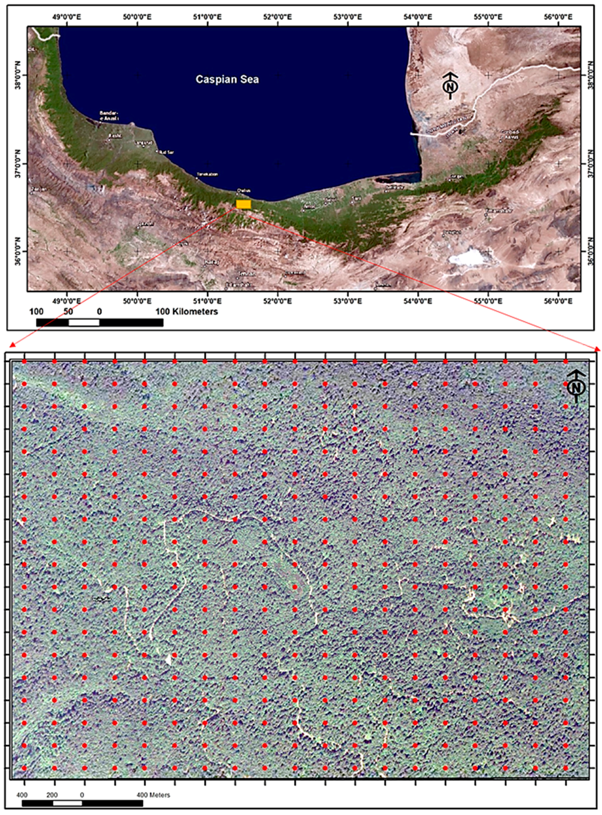
The Gorazbon forest is located about 22 km from the Caspian Sea in the north of Iran at an elevation of 1010 to 1380 meters above sea level (Figure 1). This forest is located 8 km from the port city of Nowshahr [40]. The soil of this area is karst in nature, and calsisols are the most common type. Several factors were considered in selecting the study site, including limited human interference and exploitation, representativeness of mountain Hyrcanian forests, and high biodiversity. In addition, to determine the volume increment for productivity index of the forest, plots were needed that were measured at least twice. Several potential sites that were only surveyed during one period in time could therefore not be used for this study. As a result, after several searches, the forest site of Kheyroud was selected for our study. In this study area, plot centers were recorded with a Global Navigation Satellite System (GPS) receiver with an accuracy of around 2 to 5 m. The receiver accessed a constellation of satellites signals from space that transmitted positioning and timing data, and the receiver then used these data to determine plot center locations [41]. A total of 258 circular fixed area plots of 0.1 hectares were systematically placed on a rectangular grid of 150 m × 200 m across the Gorazbon section.
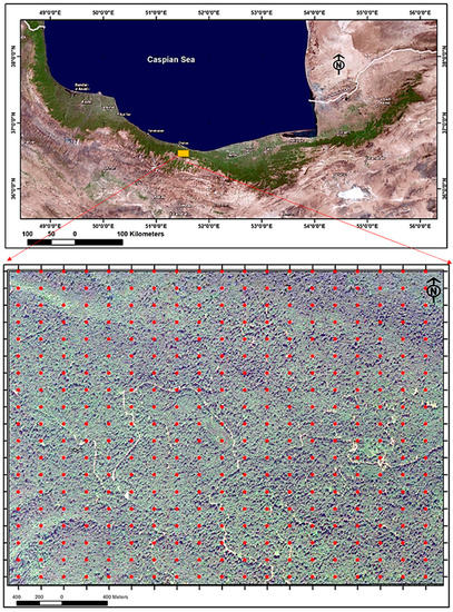
Figure 1.
The location of study area in northern Iran represents the broader boundary of the study area; the network of permanent sample plots are in the form of red dots.
The close-to-nature forest management process implemented in northern Iran has led to the development of a typical heterogeneous, uneven-aged, mixed forest within the study area (Table 1). The main tree species in the study area were Fagus orientalis Lipsky, Carpinus betulus L., Tilia platyphyllos Scop., Acer velutinum Boiss, Alnus subcordata C.A. Mey, Quercus castaeifolia C.A.M., Fraxinus excelsior L., Cerasus avium (L.) Moench, Sorbus terminalis (L.) Crantz, Ulmus glabra Hudson, Acer cappadicium Gled, Parrotia persica C.A. Mey, Diospyros lotus L. Ulmus minor Miller, Petrocarya fraxinifolia (Lam.), and Taxus baccata L. Regeneration of oriental beech (Fagus orientalis Lipsky), a preferred tree species, seems to be occurring sufficiently, even in light of competition from European hornbeam (Carpinus betulus L.) in the smaller diameter at breast height (dbh) classes [24].

Table 1.
Characteristics of the study area based on permanent forest monitoring plots in typical uneven-aged and mixed forests in northern Iran.
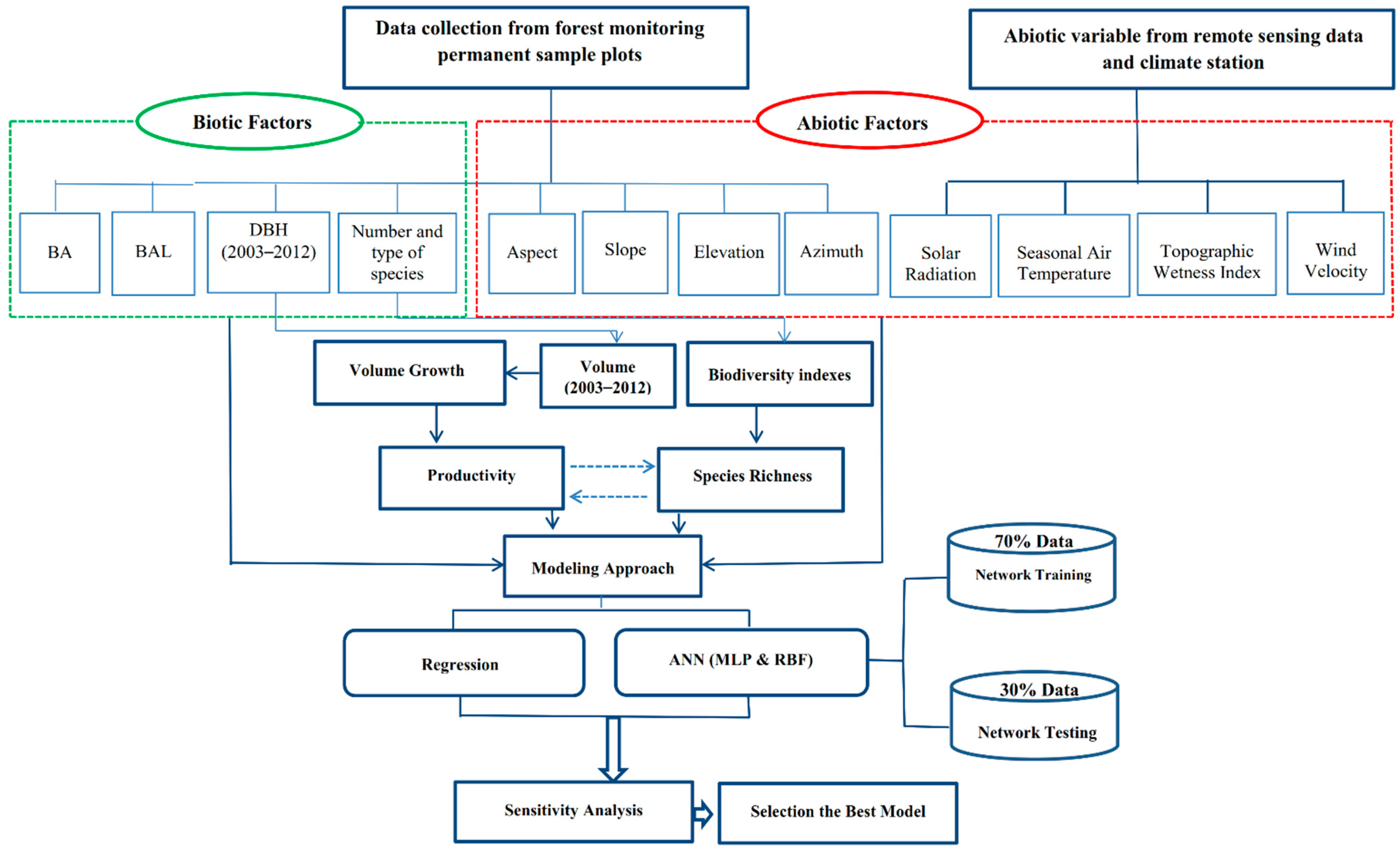
The dbh of all trees >7 cm were measured before the growing season in 2003 and again after the growing season in 2012. In both measurement periods, dbh was measured in the same manner and direction. According to the protocol explained by Bayat, Pukkala, Namiranian, and Zobeiri [40] in mixed and uneven-aged forests to obtain height curves, the height of the largest tree and the closest tree to the plot center were also determined and recorded. Using these field data, this study involved productivity (growth and yield) analysis, development of remotely sensed geographic information system (GIS databases), and modeling (Figure 2).
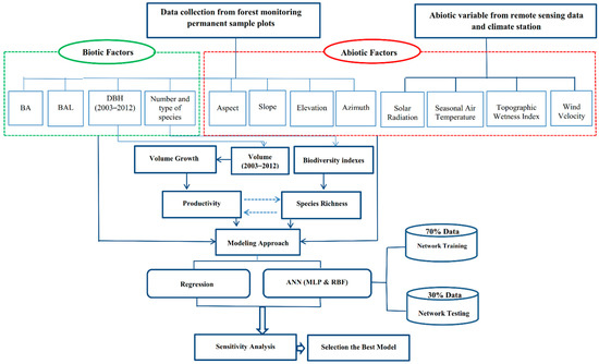
Figure 2.
A flowchart representing significant stages of the research.
2.2. Forest Productivity Analysis
The structure of the forest was quantified by using the dbh available from all trees within all permanent sample plots. We used the following functions developed for the Gorazbon forest [37] to calculate the volume of each tree in individual forest plots.
where v represents stem volume (m3), and dbh (cm) is the diameter at breast height of each tree. In order to check the accuracy of the following models, a number of cut trees were excluded from the modeling process, and their estimated volume was compared with their actual volume. In our study, productivity was assumed to be represented by the mean annual increment of the volume of trees in a forest stand (m3 ha−1 year−1). Plot estimates of mean annual increment were based on growth increment over a 9-year period (2003–2012). For both time periods, basal area and volume were computed for each tree, summed to the plot level, and extrapolated to a per-hectare estimate. In addition, the square of the basal area per hectare from 2003 was used as a variable in the modeling effort. Additionally, slope, aspect, altitude, temperature, and precipitation data associated with each permanent plot were compiled. Gross growth, including ingrowth, from 2003–2012 was calculated as follows [42]:
where VI is the average annual gross growth including ingrowth over the measurement period (2003 to 2012), VE is the volume at the end of the measurement period (2012), VH is the amount of volume that was harvested or that died between 2003 and 2012, VB is the volume at the beginning of the measurement period (2003), and years represents the length of the measurement period (9 years).
Fagus v = 0.0001000 dbh 2.503
Carpinus v = 0.0000999 dbh 2.470
Other species v = 0.0002996 dbh 2.273
VI = (VE + VH − VB)/years
2.3. Abiotic Landscape Variables
2.3.1. Solar Radiation
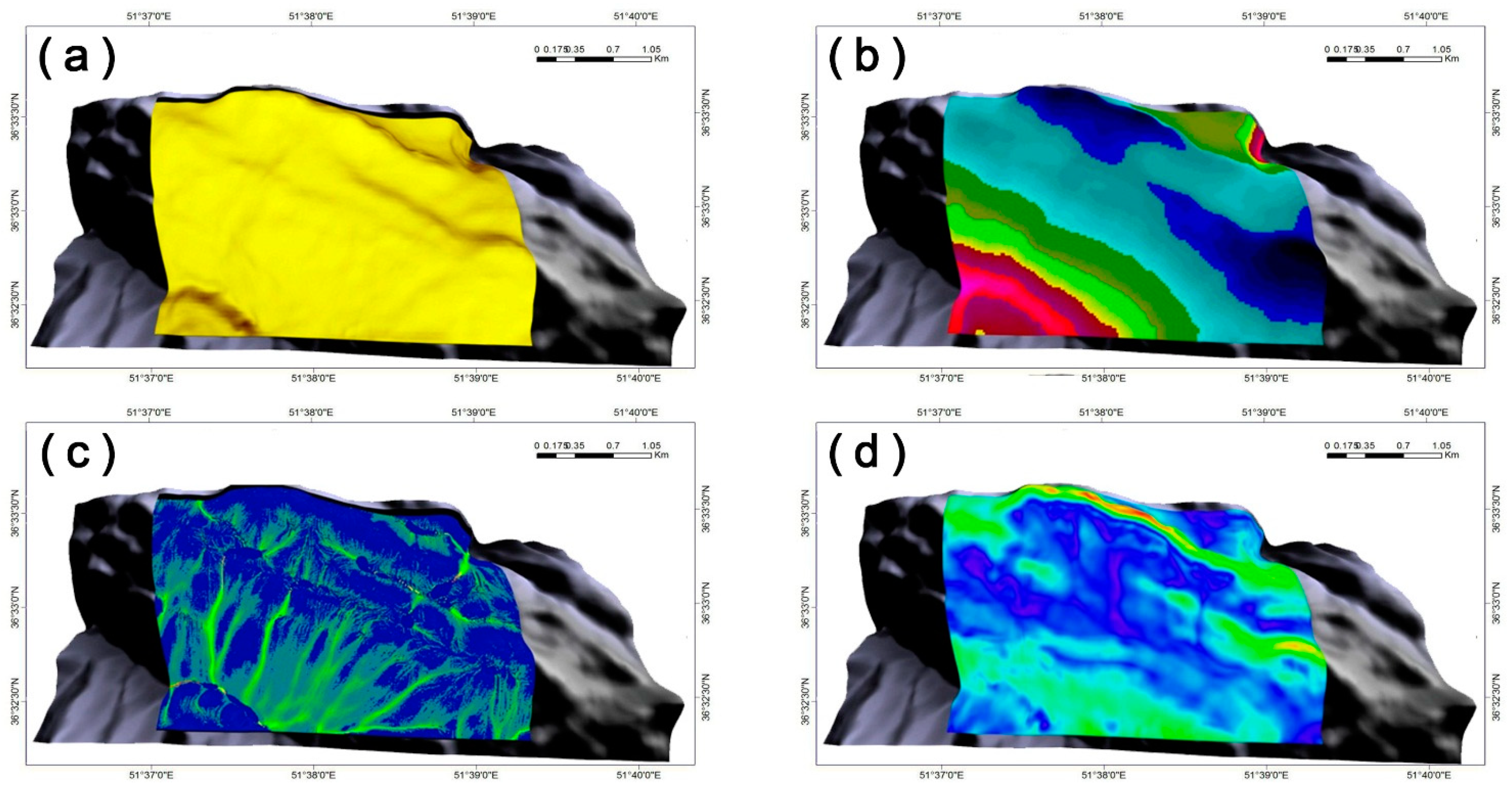
In this study, we evaluated the solar radiation as a function of (i) a digital elevation model (DEM)-based analysis that involved slope, aspect, view factor, terrain configuration factors, and horizon angle; (ii) typical solar-illumination angles and sun–earth geometry during the growing season; and (iii) solar-flux calculations at the top of the atmosphere during the growing season, based on calculations with the LanDSET (Landscape Distribution of Soil Moisture, Energy, and Temperature) model [43,44]. Ultimately, an estimate of the amount of solar radiation reaching the landscape, expressed as the growing-season cumulative cloud-free solar radiation (MJ m−2), was developed (Figure 3a).
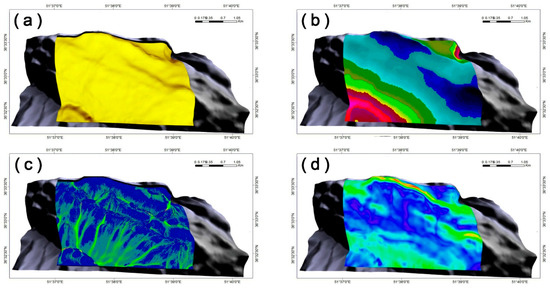
Figure 3.
Model-generated abiotic surfaces of (a) growing season cumulative cloud-free solar radiation (MJ m−2), (b) mean seasonal air temperature (°C), (c) topographic wetness index (TWI; unitless), and (d) wind velocity within the study area (m s−1).
2.3.2. Seasonal Air Temperature
As an indicator of growing season heat input, the average air temperature at different elevations across the landscape was measured [10] (Figure 3b). Both air temperature and precipitation data were interpolated from records that were obtained from the geographically closest climate stations. These data were based on records collected from 1977 to 2005, and in the interpolation process, the greatest weight was applied to data records from the closest stations (7 stations).
2.3.3. Topographic Wetness Index
In this study, prior to calculating the amount of soil water, the raw DEM was processed using the System for Automated Geoscientific Analyses (SAGA) system, an Automated Geoscientific Analyses, using the pit-filling algorithm of Planchon and Darboux [45] by removing false depressions. We then calculated the upslope contribution area in the calculation of TWI (SAGA’s modified topographic wetness index) from the mass-flux method available with the software (Figure 3c).
2.3.4. Wind Velocity
In the present study, we used a computational fluid dynamics (CFD) simulator to model wind velocity across the complex terrain of the study area (Figure 3d), which was facilitated by the DEM. CFD is a method for addressing complex three-dimensional and time-dependent relationships and can be used to numerically model various environmental variables in a virtual environment. This method is used in many fields of engineering, forestry, agriculture, etc. [33]. This model is able to accommodate three-dimensional Navier–Stokes equations, which include thermal processes and the effect of atmospheric turbulence [46,47]. The calculations are also based on a boundary-fitted coordinate system, where the initial boundary conditions are characterized by (i) average air temperature of the growing surface (as before) and wind velocity and direction (i.e., 1.7 m s−1 and 333° from true North; Figure 1) based on Nowshahr station climate records (1977–2005), and (ii) an assumed average wind velocity of 6 m s−1 at 500 m above mean sea level. Atmospheric temperature stratification is assumed neutral in the calculations (i.e., 9.86 °C km−1), a common state of the planetary boundary layer under windy and cloudy daytime conditions [48].
2.4. Biotic Variables
2.4.1. Basal Area
Basal area is a very important index in forest management and ecology and is the basis of stand structure measurements. BA was computed for each tree; then values per hectare were obtained by dividing the basal area of each plot by the total plot area (0.01 ha). These BA values per hectare are widely used for all forestry studies [24]. BA for each for each tree was calculated as follows:
where BA is basal area per tree (m2), DBH is diameter at breast height (m), and π = 3.142.
2.4.2. Basal Area in Largest Trees
The basal area in largest trees (BAL) is an index that provides an effective measure of tree dominance in a stand. It is very flexible and can easily be modified to a spatially explicit measure of competition by calculating it specifically for an influence zone around a tree. BAL is also a very suitable competition index for trees in small-sized sample plots [49]. BAL was calculated as follows:
where DBHj > DBHi (i.e., all trees larger than some assumed subject tree i), DBH is measured in meters, TFj is a tree factor, i.e., the number of trees represented by jth tree in a hectare), and π = 3.142 [50].
2.4.3. Number of Trees per Hectare
Stand density is an important indicator of stand biodiversity and one of the important indices in forest management. It is defined as the density of a stand or the number of living trees in a given area. This measurement is an indicator of the area occupied by trees and is clearly related to the structure of a stand. The number of trees in a forest stands depends on their size, which is why BA is commonly used to describe the density of a stand [51]. The number of trees per unit land area is calculated as follows:
where N is density or the number of tree per hectare, is the average number of trees in plots, and a is the area of a representative plot in hectares.
2.5. Biodiversity Indicators
In this study, we used species richness, Shannon Wiener, and Simpson indices to estimate biodiversity. Even though there may be a large number of biodiversity indicators, because some indicators are based on similar concepts, in most studies, especially in modeling, only the most important and widely used indicators are presented. Moreover, a combination of species counts (richness) and relative species abundance, which together can be viewed as indices of heterogeneity, can be very beneficial in the representation of the diversity of an ecosystem [17].
The species diversity values for each permanent sample plot were calculated using the following indicators in STATISTICA, SPSS, and Excel software:
1. Species richness index: Species richness refers to the number of species on a particular surface or specimen, regardless of the number of individuals studied in any species. The species richness index indicates the presence of different species and is obtained by counting the unique number of plant species in an area [24].
2. Heterogeneity index (heterogeneity): Heterogeneity indicators involve a combination of species richness and uniformity, and these indices summarize the two values of species richness and uniformity in a single measure. In this study, the Shannon Wiener and Simpson methods [52] were used to estimate species diversity (Table 2).
Table 2.
Biodiversity indicators used in the study (Modified after Krebs [53].
3. Modeling Approaches
3.1. Artificial Neural Network
Artificial neural networks (ANNs) are a form of artificial intelligence that involve generalizable methods for understanding relationships and, compared to other methods, are less sensitive to data outliers and noise [37]. Within an ANN, the MLP process includes neurons that are divided into layers, input and output, along with one or more hidden layers. The root mean square error (RMSE), which measures the amount of error between observations and predictions, is used in this study to validate the results. The coefficient of determination (R2) and the bias were also used along with the RMSE to evaluate the results of the ANN model (Equations (8)–(10)), as suggested by previous works [54,55].
where Psi is observed productivity, Ps is estimated productivity, is the mean of observed productivity, and is the mean of estimated productivity. A set of training and test input data is required for each network. Here, we used 70% of the dataset for network learning and the remaining 30% for testing. In this research, the number of neurons contained in the input layer and the output layer are equal to the number of input and output variables [56]. Deciding upon the number of hidden layers and the number of neurons in each hidden layer is a challenging task. In the present study, we followed the conventional trial-and-error procedure method to determine the appropriate number of hidden layers and their neurons. We used tan–sigmoid and log–sigmoid functions for the hidden layers and a linear activation function for the output layer to develop the network architecture.
Radial Basis Function (RBF) is a multilayered feedforward neural network that is similar to MLP and is used to solve classification problems. Each archive in an RBF model has two important factors that describe the location of the function’s center and its deviation or width. The distance between the input data vector and the RBF center is measured in the hidden unit, which is used along with the function’s deviation to obtain the output [57].
3.2. Poisson Regression
Poisson regression is a generalized linear model form of regression analysis used to modeling and was performed and analyzed using the stepwise method. For this analysis, the dependent variables were productivity and species richness, and the independent variables were solar radiation, air temperature, TWI, wind velocity, square of plot basal area, plot basal area, basal area in largest trees (BAL), and species richness.
3.3. Sensitivity Analysis
In the regression approach, we used stepwise regression to select the most effective factors. Using stepwise regression, we selected the most important factors that had the greatest impact on productivity. In the ANN approach, a sensitivity analysis was performed using STATISTICA software to prioritize inputs and their effectiveness in predicting outputs. By creating networks, training and testing; making sure the artificial neural network is working properly; and confirming that the network is able to accurately predict untrained data, we examined the impact of each independent input variable. In order to determine the sensitivity of each independent variable, the values of other independent variables were held constant at their nominal value (e.g., average), and the values of the tested variable were changed to determine the model response (productivity). The productivity rates were considered most sensitive to changes in each of the independent variables. This course of action was repeated for all independent variables, and an assessment was made of greatest change in productivity (increase or decrease) as a result of varying the inputs by one percent [56].
4. Results
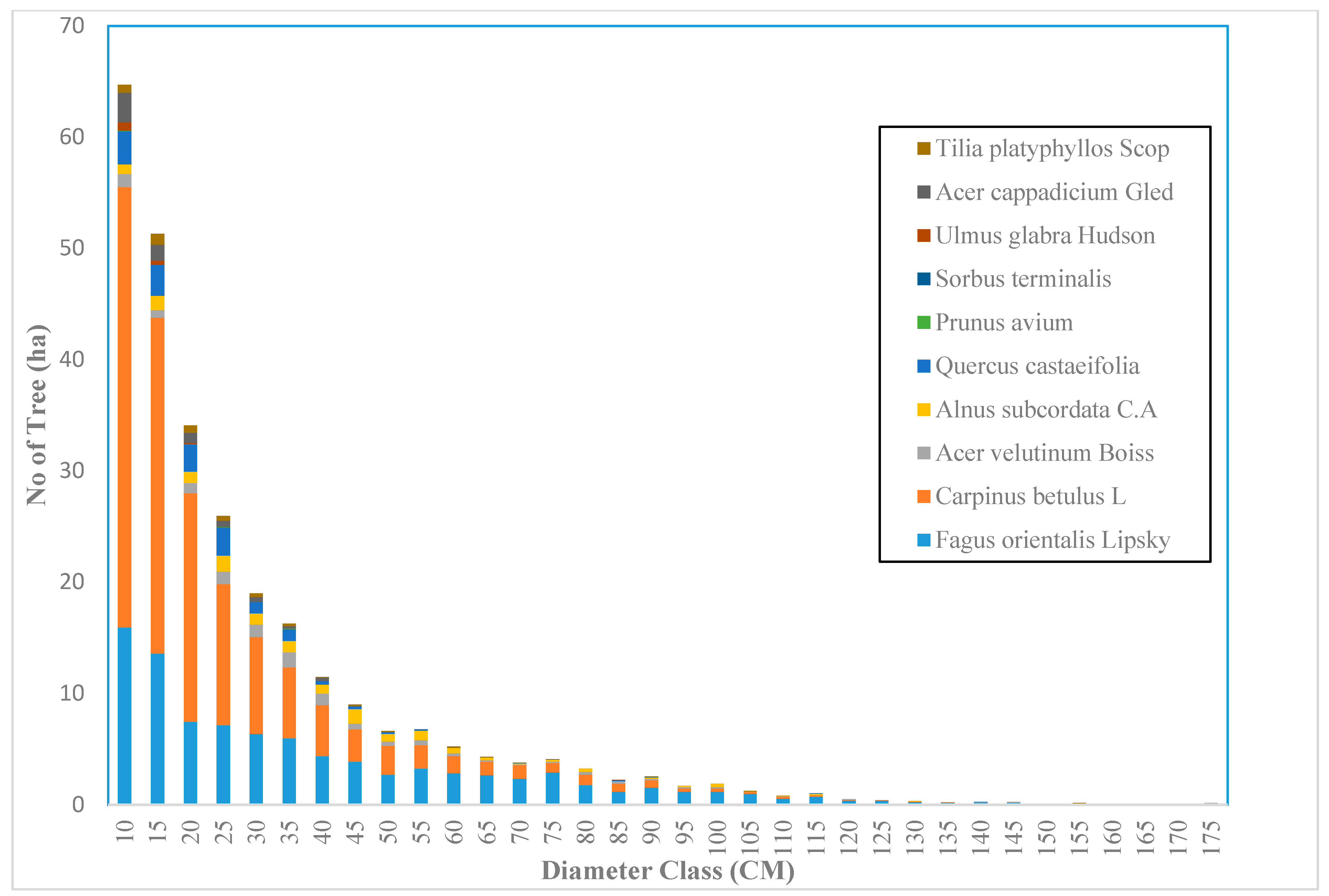
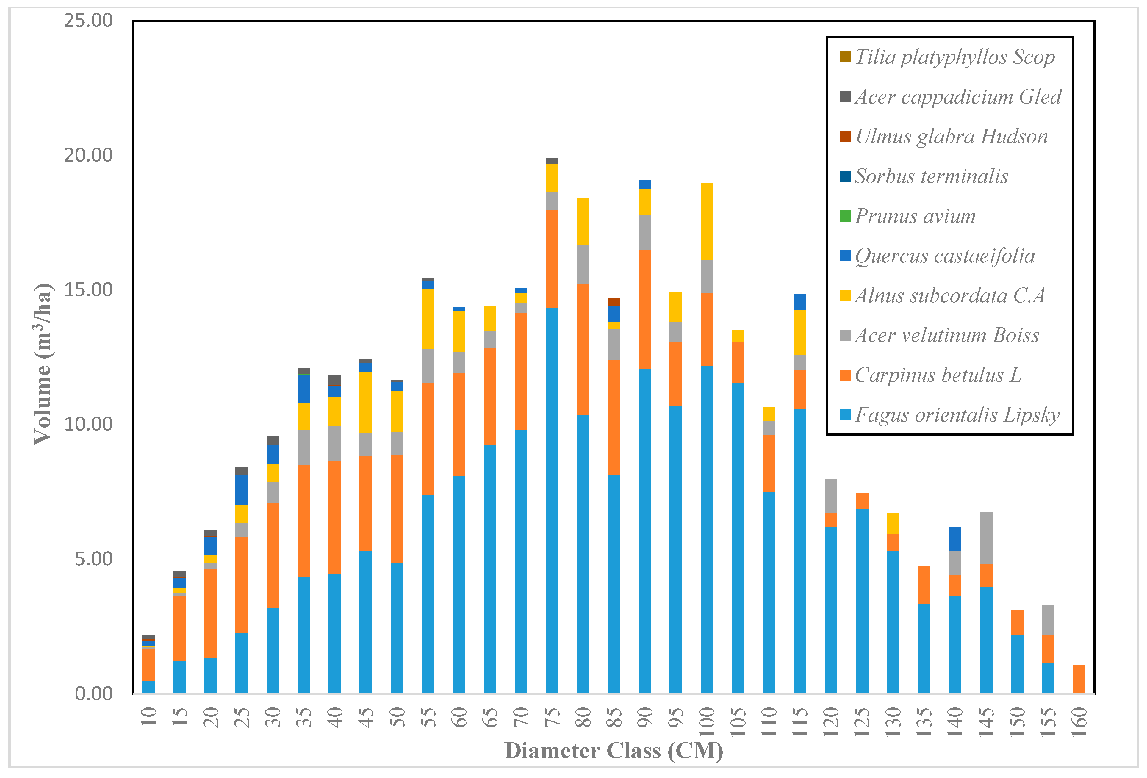
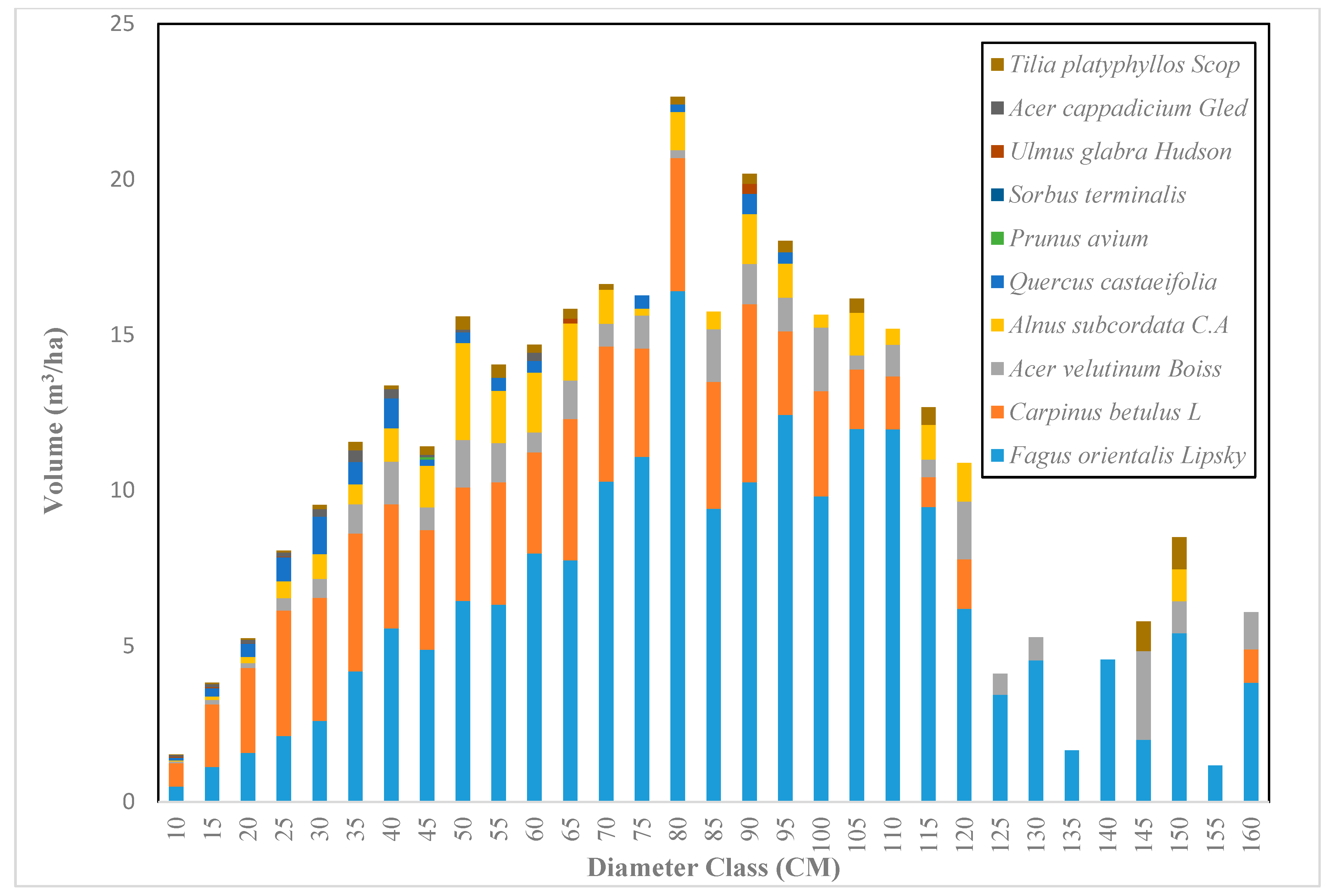
Across the sample plots, there was quite a lot of variation in tree density per ha, but interestingly, much less variation in basal area per ha. The diameter distribution of trees sampled in the study area for the first and second measurement periods describes the typical reverse J-shaped frequency distributions of uneven-aged forests (Figure 4 and Figure 5). The volume distribution by diameter class in the study area during both measurement periods indicated that oriental beech had the greatest footprint from a tree volume perspective, particularly in the higher dbh classes (Figure 6 and Figure 7). The tree species with the greatest density, European hornbeam, had high volume distributions in the smaller dbh classes. Due to the fact that volume is based on dbh and height, while there are more trees in the smaller diameter classes, larger amounts of per-hectare volume can be found in the larger diameter classes. From an analysis of the data, we determined that the average growth rate of the plots in the study area was about 4 m3 ha−1 yr−1. Interestingly, neither the shape or magnitude diameter distribution nor the shape or magnitude of the volume distribution changed much between the measurement periods.
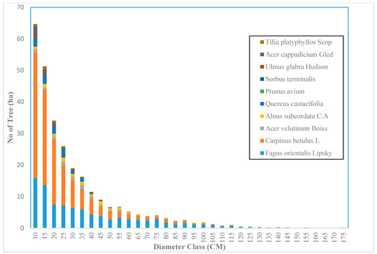
Figure 4.
The diameter distribution for uneven-aged and mixed forests in the Gorazbon section in year 2003.
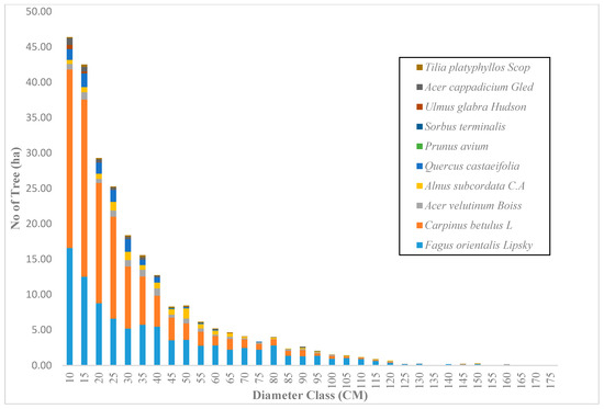
Figure 5.
The diameter distribution for uneven-aged and mixed forests in the Gorazbon section in year 2012.
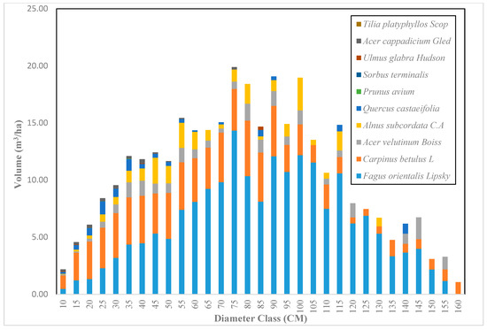
Figure 6.
The volume distribution based on diameter class in the Gorazbon section in 2003.

Figure 7.
The volume distribution based on diameter class in the Gorazbon section in 2012.
The results of regression modeling effort, using species richness as the dependent variable, are as follows (11):
where SR is the species richness, SH is Shannon Wiener index, EV is evenness, BA is the basal area (m2/ha) in 2003, and WIND is the general speed of wind in the area of the plot. The coefficient of determination (R2) of this modeled equation was 0.92, the RMSE was 0.55 m2/ha, and the relative RMSE was 17.39%. As can be seen, species richness had a significant relationship only with species evenness and Shannon Wiener index, wind velocity, and basal area. In addition, as in the above relationship, the relationship of species richness with the evenness factor is negative. This suggests that, with increasing species richness, species evenness decreased. According to field data from permanent sampling plots, in these forests, the range of Shannon Wiener index and the Simpson index was 0.5 to 1.5. A good relationship was observed between actual and modeled species richness based on the conditions within each permanent plot.
SR = 2.90 − 0.05 BA + 0.06 BA2 + 1.19 SH − 0.61 EV + 0.08 WIND
The neural network structure consisted of a multi-input layer, a hidden multilayer, and an output layer, with a minimum of 6 and a maximum of 30 layers (Table 3 and Table 4). The independent variables of BA2, BA, BAL, WIND, TWI, EV, AIRTEM, and ASOL were input layers, and the dependent variable (species richness) was the output layer. For each of the MLP- and RBF-based ANNs, five models were examined. MLP-based ANNs and RBF-based models for data collection and test data are shown with R2 = 0.94 values in Table 3 and Table 4, indicating that a strong linear relationship existed between the actual measured species richness and the predicted species richness by the MLP. Table 3 and Table 4 show the statistics for the two models RBF and MLP and the ANN model for two stages training and evaluation, respectively. For each step, 10 models are used, and in these tables, the selected models are highlighted based on their low RMSE and bias values. With respect to model training and valuation, the multilayer perceptron (MLP 10-6-1 with R2 = 0.94 and RMSE = 0.008) model was noted as being the most effective at predicting species richness.
Table 3.
Characteristics of RBF and MLP-based ANNs and associated metrics for SR model training.
Table 4.
Characteristics of RBF and MLP-based ANNs and associated metrics for SR model evaluation.
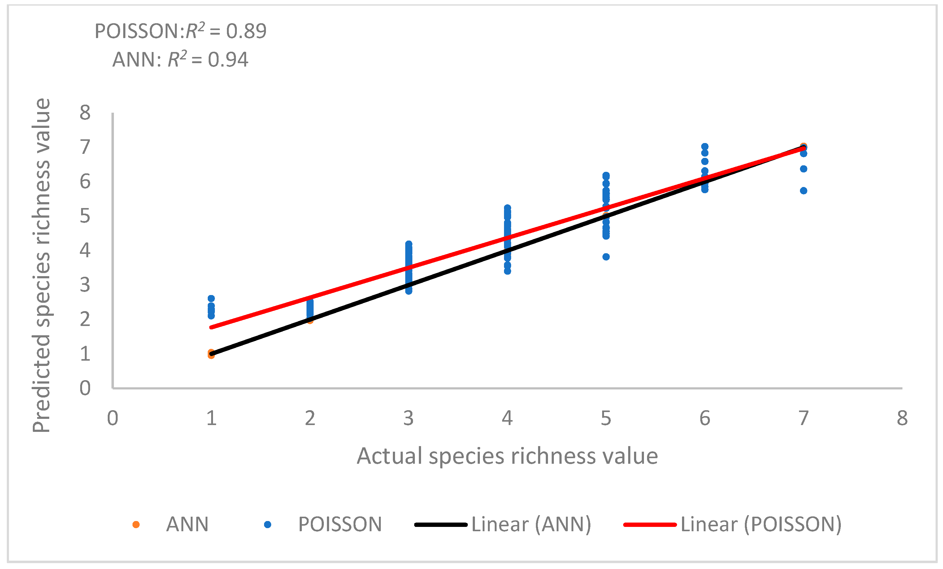
The relationship between the actual and predicted species richness when the ANN model was used was strong (Figure 8). However, the relationship between actual and predicted species richness from the two models (regression and ANN) suggests that the ANN model was more capable in predicting species richness. The influential factors in this method are the following variables: EV, BA2, BA, TWI, AIRTEM, WIND, and ASOL.
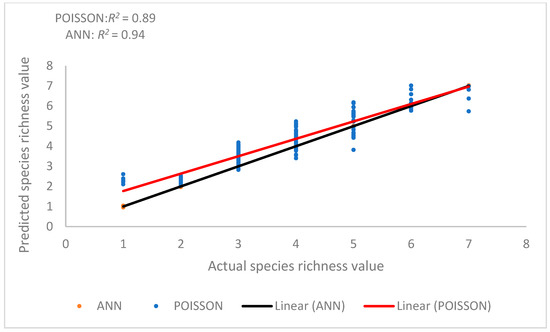
Figure 8.
Relationship between predicted and actual SR values Poisson regression (red line), and nonparametric methods (ANN (black line)).
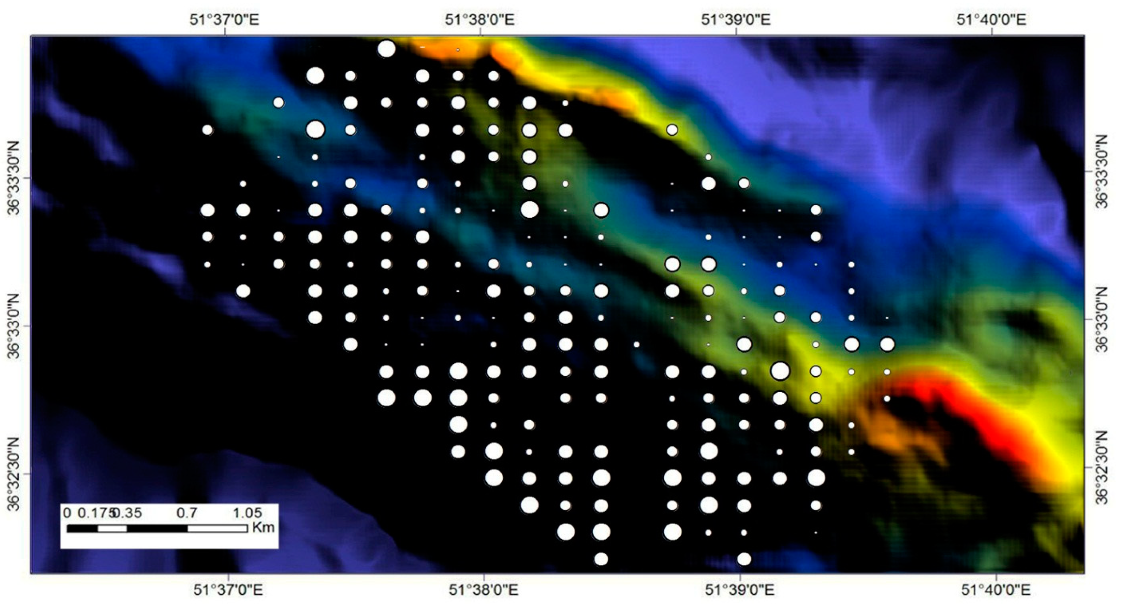
With respect to the field plots, species diversity varied considerably across the landscape. The size of the points representing the locations of the field plots were scaled according to the Shannon Wiener index values of each plot (Figure 9). Larger points represent higher index values, and smaller points represent lower index values. The range of the index was about 0.1 to 1.5.

Figure 9.
Spatial variation of tree species diversity at the plot level, which is estimated according to the Shannon Wiener index. The large circles coincide with high index values (high species diversity with an upper value of 1.6), whereas small circles coincide to low values (low species diversity with a lower value of 0.1).
The following relationship is the regression model developed to estimate productivity from the independent variables in the study area (12):
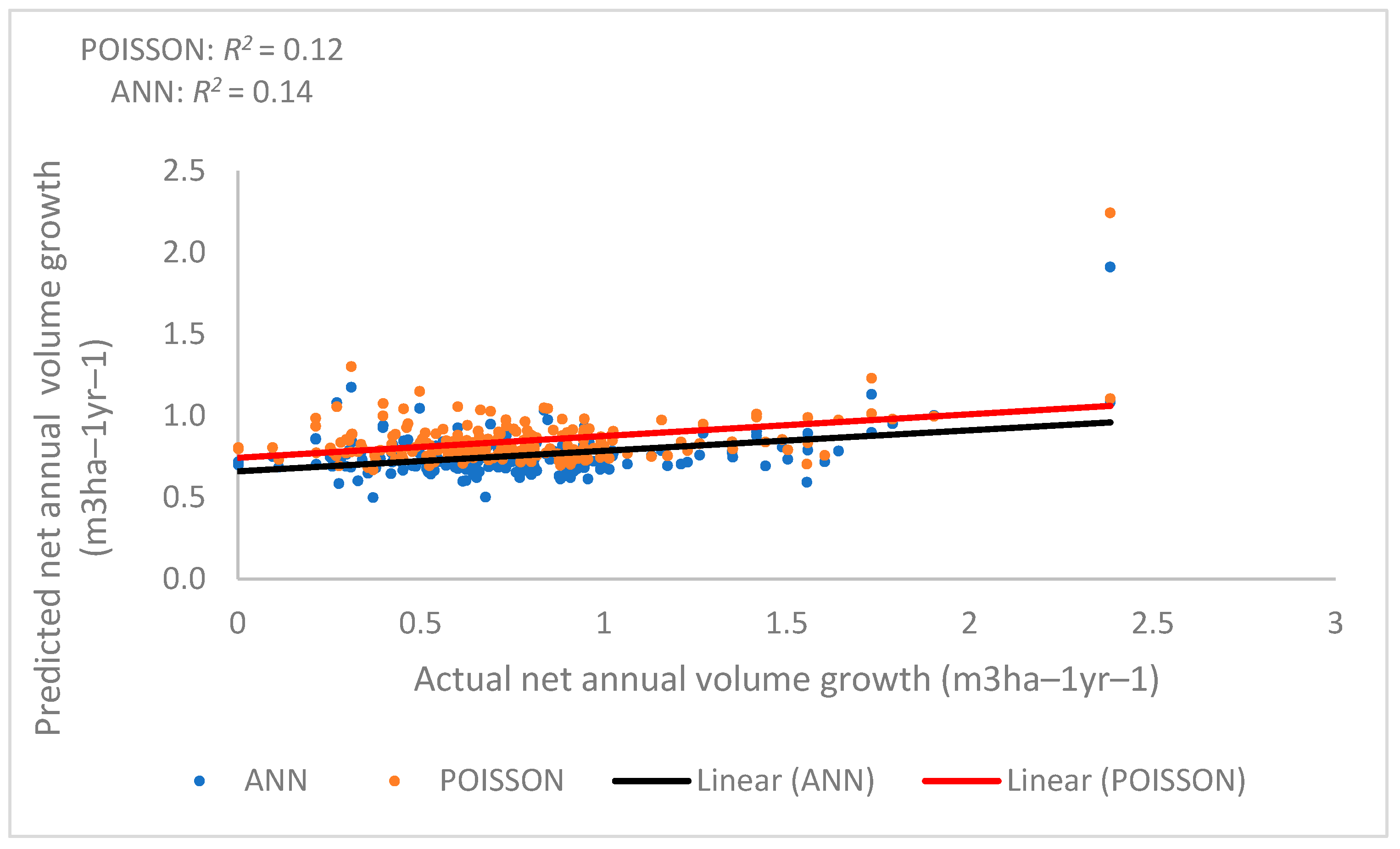
where P is productivity, the 9-year net annual volume growth (m3/ha); BA is the basal area (m2/ha) in 2003; and WIND is the general speed of wind in the area of the plot. BA (t = −3.90, p = 0.00013), BA2 (t = 4.73, p = 0.00000413), and WIND (t = 2.32, p = 0.021) were statistically significant components of the model. The net annual volume growth model using the regression method had an R2 of 0.20, a RMSE of 0.41 m3 ha−1, a BIAS of 0.0035 m3 ha−1, a relative RMSE of 48.63%, and a relative BIAS of 0.55%. In summary, this method for estimating productivity based on biological and environmental variables was not very good. Figure 10 shows the relationship between actual net annual volume growth (m3 ha−1 year−1) and predicted net annual volume growth (m3 ha−1 year−1). This suggests that predicting net annual growth from the actual growth of these forests is difficult using a regression model.
P = 0.943 − 0.02181 BA + 0.02787 BA2 + 0.03732 WIND + 0.002 SR
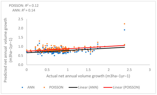
Figure 10.
Relationship between predicted and actual net annual volume growth (productivity) by (Poisson regression (red line) and nonparametric methods (ANN (black line)).
When using the ANN, a minimum of 4 layers and a maximum of 27 hidden layers were used. The results show that when 12 hidden layers were used, the highest accuracy can be estimated (Table 5 and Table 6). While the RMSE and bias were low, MLP-based ANNs and RBF-based models had moderately good coefficient of determination values (R2 = 0.34 for the selected model), indicating that a fair linear relation existed between the actual measured net annual volume growth and the predicted net annual volume growth.
Table 5.
Characteristics of RBF and MLP-based ANNs and associated metrics for productivity model training.
Table 6.
Characteristics of RBF and MLP-based ANNs and associated metrics for productivity model evaluation.
According to the sensitivity analysis, a species enrichment factor of 31% had the greatest effect on productivity and biotic and abiotic factors including square of plot basal area, plot basal area, wind velocity, air temperature, ASOl, and TWI, which had 15.9%, 13.3%, 10.3%, 9.8%, 9.8%, and 10% effects, respectively. Therefore, it can be said that, in total, species richness (31%), total biotic factors (about 29%), and total abiotic factors (about 40%) described the variation of productivity. Table 7 shows the results of the sensitivity analysis for the best model to illustrate the effect of biotic, abiotic factors, and species richness on productivity.
Table 7.
Percent impact of individual and grouped variables (species richness and abiotic and biotic factors) on MLP-based calculations of productivity according to the sensitive analysis.
5. Discussion
In this study, the results suggest that there is a positive and significant relationship between species richness and forest productivity in the study area. Productivity estimates based on the ANN and regression models illustrated the role of species richness as an influential factor in estimating productivity. However, this relationship was stronger and more meaningful in the results from the ANN model. Based on the modeling results, forest productivity in the study area was largely dependent on nonbiological factors such as wind velocity and TWI. The results of this study are consistent with other studies that have concluded there is a significant relationship between productivity and forest biodiversity, ranging from regional to global scales [2,58].
The predominant forest management system employed in this study area has been close-to-nature management of forests, and this has caused these forests to become uneven-aged over time. The use of this forest management system has resulted in mixed and heterogeneous stands of tree species. In such forests, there may be a higher resistance to change caused by biotic and abiotic factors and events such as insects, disease, droughts, or storms [59,60,61,62]. In mixed stands, different tree species occupy different niches. These types of forests can be more resistant to change because they possess different tolerances against environmental disturbances. Among the important factors affecting species richness in the study area were wind velocity and topographic wetness index. Wind velocity, alone, explained much of the richness of species. This result is consistent with the findings of Bourque and Bayat [22] in the Kheyroud forest, which examined changes in the landscape on biodiversity. In that study, wind velocity, surface reflection of blue light, height of land above the nearest drainage point, and TWI had the greatest effects on the species richness. Wind speed has also been shown to provide favorable conditions for the growth of beech species [23]. For example, wind speed can exert either a positive or a negative physiological and biomechanical effect on plants. In a low wind velocity environment, the transfer of carbon dioxide to plants can be hindered due to the large boundary layer resistances that exist, and this can result in decreased growth rates for the plants that are affected [35]. In addition, in a high wind velocity environment, permanent deformation of plants can occur, as wind can distort growing patterns through application of constant bending pressures. Further, it may be observed that an increase in the transfer of water vapor from plants to the atmosphere has occurred in this type of environment, causing the closure of leaf stomata to help prevent desiccation. In this latter case, uptake of CO2 may be reduced, negatively affecting plant growth. As a result, the optimal growing conditions based on wind velocity occur somewhere in between these extremes [22,23].
In terms of productivity prediction models, species richness was one of the important factors and had a stronger presence in the ANN model. However, according to sensitivity analysis, the most important and influential factor in this regard was the BA, while abiotic factors such as TWI, wind speed, and solar radiation were also important in later stages. This result is in line with the findings of Bayat et al. [32], who studied factors affecting the growth of beech diameter in the forests of northern Iran. However, the regression analysis produced a nonlinear model that was better able to predict growth based solely on basal area. The relationship between species richness and productivity in the study area can be explained by, among other things, the dominant species in an area being the most fertile species. This is the effect of natural selection. More importantly, the richness of the species leads to the division of niches between the six species, which creates a wide range of functional strategies between species. As a result, this can be the main and important process in the relationship between species richness and productivity in a forest [63,64]. Another important factor that can justify this relationship is that higher species diversity has led to higher structural complexity that indirectly affects biomass, and, as it has been proven, forests with higher carbon storage potential also have higher biodiversity potential [65]. It is also important to note that the relationship between productivity and biodiversity can change with spatial scale and climate. As various studies have shown, this relationship has been stronger in boreal forests and less or even meaningless in temperate forests [8,20].
Huang et al. [19]; Paquette and Messier [8]; and Rita and Borghetti [20], in their studies in Chinese, Canadian, and Italian forests, concluded that the richness of the species has a strong effect on forest productivity, and in these diverse environments, coexisting species can have different niches and competitiveness. Biodiversity and its various effects have also been reported to be much stronger in boreal biomes than in temperate regions [63]. In boreal environments where environmental conditions are more extreme, disturbances are more intense, and tensions are higher, the interactions between species may be more important and decisive Paquette and Messier [8]. Therefore, these reasons can justify the relative low effect of biodiversity on productivity in the study area.
In this study, it was observed that ANN models, based on criteria for evaluating models such as RMSE and coefficient of determination, were more accurate than regression models and showed better relationships between productivity and biodiversity in the studied forest. As the results showed, they are in line with the findings of other research [32,66,67]. The ANN of the multilayer perceptron (MLP) type had good ability in prediction and estimation of productivity in our forests. With respect to species richness, Model 4, which had 10 inputs, 6 hidden layers, and 1 output, had the highest R2 (0.94) and the lowest RMSE (0.75) and was selected as the best SR predictor model. With respect to forest productivity, MLP Model 2 with 10 inputs, 12 hidden layers, and 1 output, had R2 and RMSE of 0.34 and 0.42, respectively, representing the best model. Both of these used a logistic function.
Therefore, it can be said that the nonlinear and complex nature of the relationship between biodiversity and forest productivity may be better described using neural network models. However, each modeling method has its own set of strengths and weaknesses. In regression models, the relationship between variables is simple, yet assumptions such as normality of data, independence of variables, and many other conditions are limitations on the use of these models [32]. Bayat, Bettinger, Heidari, Henareh Khalyani, Jourgholami, and Hamidi [67] used comparative regression and artificial intelligence methods to conclude that artificial intelligence methods such as neural networks have a higher ability and accuracy in determining height in these forests. Artificial intelligence-based models such as neural networks do not have the same limitations as regression models and have the ability to work with qualitative variables. The results of various studies show that they can have a relatively high accuracy in predicting different conditions of a forest [68].
6. Conclusions
In areas with adequate precipitation and increasing air temperatures, competition between plant species will intensify when external pressures are eliminated, and for society, a discussion of biodiversity and its effects on forest productivity will be of particular importance. In this study, the relationship between tree species richness and various biotic and abiotic variables in the forests of northern Iran was examined. The results showed a strong relationship between species richness and wind speed and topographic wetness index factors. Furthermore, the relationship between forest productivity and biotic and abiotic factors was examined. In this case, species richness, basal area, and wind speed played important roles in understanding changes in productivity, and the role of species richness in describing the variability in productivity was significant. In this regard, the results of this study are consistent with the findings of other studies that have shown that the relationship between productivity and species richness in temperate forests can be strong. Through regression analysis, we also showed that a nonlinear model was able to predict growth based solely on basal area. In summary, forest productivity seems to be more affected by environmental variables and local site conditions. However, according to a sensitivity analysis, species diversity had significant and positive effects on productivity in species-rich broadleaved forests, but the effects of biotic and abiotic factors were also important. The ANN models that were developed were more capable than regression models of describing the relationships between species richness and productivity when using abiotic environmental factors.
Author Contributions
M.B. conceived and designed the experiments; M.B. and S.H. performed the experiments and analyzed the data; M.B. and S.K.H. contributed reagents/materials/analysis tools; M.B., P.B. and A.J. wrote the paper. All authors have read and agreed to the published version of the manuscript.
Funding
This research received no external funding.
Institutional Review Board Statement
Not applicable.
Informed Consent Statement
Not applicable.
Data Availability Statement
The data underlying this article will be shared on reasonable request to the corresponding author.
Conflicts of Interest
None of the authors have any actual or potential conflict of interest that could inappropriately influence, or be perceived to influence, this work.
References
- Zhang, Y.; Chen, H.Y.; Reich, P.B. Forest Productivity Increases with Evenness, Species Richness and Trait Variation: A Global Meta-Analysis. J. Ecol. 2012, 100, 742–749. [Google Scholar] [CrossRef]
- Liang, J.; Crowther, T.W.; Picard, N.; Wiser, S.; Zhou, M.; Alberti, G.; Schulze, E.-D.; McGuire, A.D.; Bozzato, F.; Pretzsch, H.; et al. Positive Biodiversity-Productivity Relationship Predominant in Global Forests. Science 2016, 354, aaf8957. [Google Scholar] [CrossRef] [PubMed] [Green Version]
- Jactel, H.; Gritti, E.S.; Drössler, L.; Forrester, D.I.; Mason, W.L.; Morin, X.; Pretzsch, H.; Castagneyrol, B. Positive Biodiversity–Productivity Relationships in Forests: Climate Matters. Biol. Lett. 2018, 14, 20170747. [Google Scholar] [CrossRef]
- Ratcliffe, S.; Wirth, C.; Jucker, T.; van der Plas, F.; Scherer-Lorenzen, M.; Verheyen, K.; Allan, E.; Benavides, R.; Bruelheide, H.; Ohse, B. Biodiversity and Ecosystem Functioning Relations in European Forests Depend on Environmental Context. Ecol. Lett. 2017, 20, 1414–1426. [Google Scholar] [CrossRef] [PubMed]
- Ouyang, S.; Xiang, W.; Wang, X.; Xiao, W.; Chen, L.; Li, S.; Sun, H.; Deng, X.; Forrester, D.I.; Zeng, L.; et al. Effects of Stand Age, Richness and Density on Productivity in Subtropical Forests in China. J. Ecol. 2019, 107, 2266–2277. [Google Scholar] [CrossRef]
- Tilman, D.; Knops, J.; Wedin, D.; Reich, P.; Ritchie, M.; Siemann, E. The Influence of Functional Diversity and Composition on Ecosystem Processes. Science 1997, 277, 1300–1302. [Google Scholar] [CrossRef] [Green Version]
- Hooper, D.U.; Chapin, F.S.; Ewel, J.J.; Hector, A.; Inchausti, P.; Lavorel, S.; Lawton, J.H.; Lodge, D.M.; Loreau, M.; Naeem, S.; et al. Effects of Biodiversity on Ecosystem Functioning: A Consensus of Current Knowledge. Ecol. Monogr. 2005, 75, 3–35. [Google Scholar] [CrossRef]
- Paquette, A.; Messier, C. The Effect of Biodiversity on Tree Productivity: From Temperate to Boreal Forests. Glob. Ecol. Biogeogr. 2011, 20, 170–180. [Google Scholar] [CrossRef] [Green Version]
- Barrufol, M.; Schmid, B.; Bruelheide, H.; Chi, X.; Hector, A.; Ma, K.; Michalski, S.; Tang, Z.; Niklaus, P.A. Biodiversity Promotes Tree Growth during Succession in Subtropical Forest. PLoS ONE 2013, 8, e81246. [Google Scholar] [CrossRef] [Green Version]
- Shen, X.; Liu, B.; Jiang, M.; Lu, X. Marshland Loss Warms Local Land Surface Temperature in China. Geophys. Res. Lett. 2020, 47. [Google Scholar] [CrossRef] [Green Version]
- Poorter, L.; van der Sande, M.T.; Thompson, J.; Arets, E.J.; Alarcón, A.; Álvarez-Sánchez, J.; Ascarrunz, N.; Balvanera, P.; Barajas-Guzmán, G.; Boit, A. Diversity Enhances Carbon Storage in Tropical Forests. Glob. Ecol. Biogeogr. 2015, 24, 1314–1328. [Google Scholar] [CrossRef]
- Forrester, D.I.; Bauhus, J. A Review of Processes Behind Diversity—Productivity Relationships in Forests. Curr. For. Rep. 2016, 2, 45–61. [Google Scholar] [CrossRef] [Green Version]
- Seidel, D.; Leuschner, C.; Scherber, C.; Beyer, F.; Wommelsdorf, T.; Cashman, M.; Fehrmann, L. The Relationship between Tree Species Richness, Canopy Space Exploration and Productivity in a Temperate Broad-Leaf Mixed Forest. For. Ecol. Manag. 2013, 310, 366–374. [Google Scholar] [CrossRef]
- Chen, X.; Quan, Q.; Zhang, K.; Wei, J. Spatiotemporal Characteristics and Attribution of Dry/Wet Conditions in the Weihe River Basin Within a Typical Monsoon Transition Zone of East Asia over the Recent 547 Years. Environ. Model. Softw. 2021, 143, 105116. [Google Scholar] [CrossRef]
- Zhang, K.; Ali, A.; Antonarakis, A.; Moghaddam, M.; Saatchi, S.; Tabatabaeenejad, A.; Chen, R.; Jaruwatanadilok, S.; Cuenca, R.; Crow, W.T.; et al. The Sensitivity of North American Terrestrial Carbon Fluxes to Spatial and Temporal Variation in Soil Moisture: An Analysis Using Radar-Derived Estimates of Root-Zone Soil Moisture. J. Geophys. Res. Biogeosci. 2019, 124, 3208–3231. [Google Scholar] [CrossRef]
- Peet, R.K. The Measurement of Species Diversity. Annu. Rev. Ecol. Syst. 1974, 5, 285–307. [Google Scholar] [CrossRef]
- Yeom, D.-J.; Kim, J.H. Comparative Evaluation of Species Diversity Indices in the Natural Deciduous Forest of Mt. Jeombong. For. Sci. Technol. 2011, 7, 68–74. [Google Scholar] [CrossRef]
- Loreau, M.; Hector, A.L. Partitioning Selection and Complementarity in Biodiversity Experiments. Nat. Cell Biol. 2001, 412, 72–76. [Google Scholar] [CrossRef]
- Huang, Y.; Chen, Y.; Castro-Izaguirre, N.; Baruffol, M.; Brezzi, M.; Lang, A.; Li, Y.; Härdtle, W.; von Oheimb, G.; Yang, X.; et al. Impacts of Species Richness on Productivity in a Large-Scale Subtropical Forest Experiment. Science 2018, 362, 80–83. [Google Scholar] [CrossRef] [PubMed] [Green Version]
- Rita, A.; Borghetti, M. Linkage of Forest Productivity to Tree Diversity under Two Different Bioclimatic Regimes in Italy. Sci. Total Environ. 2019, 687, 1065–1072. [Google Scholar] [CrossRef]
- Yang, S.-I.; Burkhart, H.E. Evaluation of Total Tree Height Subsampling Strategies for Estimating Volume in Loblolly Pine Plantations. For. Ecol. Manag. 2020, 461, 117878. [Google Scholar] [CrossRef]
- Bourque, C.P.-A.; Bayat, M. Landscape Variation in Tree Species Richness in Northern Iran Forests. PLoS ONE 2015, 10, e0121172. [Google Scholar] [CrossRef]
- Bourque, C.P.-A.; Bayat, M.; Zhang, C. An Assessment of Height–Diameter Growth Variation in an Unmanaged Fagus Orientalis-Dominated Forest. Eur. J. For. Res. 2019, 138, 607–621. [Google Scholar] [CrossRef]
- Bayat, M.; Burkhart, H.; Namiranian, M.; Hamidi, S.; Heidari, S.; Hassani, M. Assessing Biotic and Abiotic Effects on Biodiversity Index Using Machine Learning. Forests 2021, 12, 461. [Google Scholar] [CrossRef]
- Bourque, C.P.-A.; Gachon, P.; MacLellan, B.R.; MacLellan, J.I. Projected Wind Impact on Abies balsamea (Balsam fir)-Dominated Stands in New Brunswick (Canada) Based on Remote Sensing and Regional Modelling of Climate and Tree Species Distribution. Remote Sens. 2020, 12, 1177. [Google Scholar] [CrossRef] [Green Version]
- Pilli, R.; Pase, A. Forest Functions and Space: A Geohistorical Perspective of European Forests. Iforest Biogeosci. For. 2018, 11, 79–89. [Google Scholar] [CrossRef] [Green Version]
- Kwon, Y.; Lee, T.; Lang, A.; Burnette, D. Assessment on Latitudinal Tree Species Richness Using Environmental Factors in The Southeastern United States. PeerJ 2019, 7, e6781. [Google Scholar] [CrossRef] [PubMed] [Green Version]
- Oliver, C.D.; Larson, B.C. Forest Stand Dynamics: Updated Edition; John Wiley & Sons: Hoboken, NJ, USA, 1996. [Google Scholar]
- Smith, V.C.; Ennos, A.R. The Effects of Air Flow and Stem Flexure on the Mechanical and Hydraulic Properties of the Stems of Sunflowers Helianthus Annuus L. J. Exp. Bot. 2003, 54, 845–849. [Google Scholar] [CrossRef] [PubMed]
- Thomas, S.C.; Martin, A.R.; Mycroft, E.E. Tropical Trees in a Wind-Exposed Island Ecosystem: Height-Diameter Allometry and Size at Onset of Maturity. J. Ecol. 2015, 103, 594–605. [Google Scholar] [CrossRef] [Green Version]
- Wykoff, W. User's Guide to the Stand Prognosis Model; U.S. Department of Agriculture, Forest Service, Intermountain Forest and Range Experiment Station: Ogden, UT, USA, 1982; Volume 133, 112p.
- Bayat, M.; Ghorbanpour, M.; Zare, R.; Jaafari, A.; Pham, B.T. Application of Artificial Neural Networks for Predicting Tree Survival and Mortality in the Hyrcanian forest of Iran. Comput. Electron. Agric. 2019, 164. [Google Scholar] [CrossRef]
- Bayat, M.; Noi, P.T.; Zare, R.; Bui, D.T. A Semi-Empirical Approach Based on Genetic Programming for the Study of Biophysical Controls on Diameter-Growth of Fagus Orientalis in Northern Iran. Remote Sens. 2019, 11, 1680. [Google Scholar] [CrossRef] [Green Version]
- Goudriaan, J. Crop Micrometeorology: A Simulation Study; Centre for Agricultural Publishing and Documentation: Wageningen, The Netherlands, 1997; 262p. [Google Scholar]
- Bang, C.; Sabo, J.L.; Faeth, S.H. Reduced Wind Speed Improves Plant Growth in a Desert City. PLoS ONE 2010, 5, e11061. [Google Scholar] [CrossRef] [PubMed]
- Kweon, D.; Comeau, P.G. Relationships between Tree Survival, Stand Structure and Age in Trembling Aspen Dominated Stands. For. Ecol. Manag. 2019, 438, 114–122. [Google Scholar] [CrossRef]
- Hamidi, S.K.; Weiskittel, A.; Bayat, M.; Fallah, A. Development of Individual Tree Growth and Yield Model Across Multiple Contrasting Species Using Nonparametric and Parametric Methods in the Hyrcanian Forests of Northern Iran. Eur. J. For. Res. 2021, 140, 421–434. [Google Scholar] [CrossRef]
- Aertsen, W.; Kint, V.; van Orshoven, J.; Özkan, K.; Muys, B. Comparison and Ranking of Different Modelling Techniques for Prediction of Site Index in Mediterranean Mountain Forests. Ecol. Model. 2010, 221, 1119–1130. [Google Scholar] [CrossRef]
- Hamidi, S.K.; Zenner, E.K.; Bayat, M.; Fallah, A. Analysis of Plot-Level Volume Increment Models Developed from Machine Learning Methods Applied to an Uneven-Aged Mixed Forest. Ann. For. Sci. 2021, 78, 4. [Google Scholar] [CrossRef]
- Bayat, M.; Pukkala, T.; Namiranian, M.; Zobeiri, M. Productivity and Optimal Management of the Uneven-Aged Hardwood Forests of Hyrcania. Eur. J. For. Res. 2013, 132, 851–864. [Google Scholar] [CrossRef]
- Bettinger, P.; Merry, K.; Bayat, M.; Tomaštík, J. GNSS Use in Forestry—A Multi-National Survey from Iran, Slovakia and Southern USA. Comput. Electron. Agric. 2019, 158, 369–383. [Google Scholar] [CrossRef]
- Beers, T.W. Components of Forest Growth. J. For. 1962, 60, 245–248. [Google Scholar]
- Bourque, C.P.-A.; Gullison, J.J. A Technique to Predict Hourly Potential Solar Radiation and Temperature for a Mostly Unmonitored Area in the Cape Breton Highlands. Can. J. Soil Sci. 1998, 78, 409–420. [Google Scholar] [CrossRef]
- Zhao, F.; Zhang, S.; Du, Q.; Ding, J.; Luan, G.; Xie, Z. Assessment of the Sustainable Development of Rural Minority Settlements Based on Multidimensional Data and Geographical Detector Method: A Case Study in Dehong, China. Socio-Economic Plan. Sci. 2021, 101066. [Google Scholar] [CrossRef]
- Planchon, O.; Darboux, F. A Fast, Simple and Versatile Algorithm to Fill the Depressions of Digital Elevation Models. CATENA 2002, 46, 159–176. [Google Scholar] [CrossRef]
- Lopes, A. WindStation—A Software for the Simulation of Atmospheric Flows over Complex Topography. Environ. Model. Softw. 2003, 18, 81–96. [Google Scholar] [CrossRef]
- Miao, R.; Qiu, X.; Guo, M.; Musa, A.; Jiang, D. Accuracy of Space-for-Time Substitution for Vegetation State Prediction Following Shrub Restoration. J. Plant Ecol. 2018. [CrossRef] [Green Version]
- Geiger, R.; Aron, R.H.; Todhunter, P. The Climate Near the Ground; Rowman & Littlefield: Lanham, MD, USA; Vieweg+Teubner Verlag: Berlin, Germany, 2009; 528p. [Google Scholar]
- Burkhart, H.E.; Tomé, M. Modeling Forest Trees and Stands; Springer Science & Business Media: Berlin/Heidelberg, Germany, 2012; 458p. [Google Scholar]
- Pokharel, B.; Dech, J. Mixed-Effects Basal Area Increment Models for Tree Species in the Boreal Forest of Ontario, Canada Using an Ecological Land Classification Approach to Incorporate Site Effects. Forestry 2012, 85, 255–270. [Google Scholar] [CrossRef] [Green Version]
- Oyebade, B.; Eguakun, F.; Duru, B. Tree Basal Area Models and Density for Selected Plantation Species in Swamp Forest Zone of Rivers State, Nigeria. World News Nat. Sci. 2020, 30. [Google Scholar]
- Keylock, C.J. Simpson Diversity and the Shannon-Wiener Index as Special Cases of a Generalized Entropy. Oikos 2005, 109, 203–207. [Google Scholar] [CrossRef]
- Krebs, C.J. Ecological Methodology; Benjamin-Cummins Publishing CO: San Francisco, CA, USA, 1999. [Google Scholar]
- Li, J.; Zhao, Y.; Zhang, A.; Song, B.; Hill, R.L. Effect of Grazing Exclusion on Nitrous Oxide Emissions during Freeze-Thaw Cycles in a Typical Steppe of Inner Mongolia. Agric. Ecosyst. Environ. 2021, 307, 107217. [Google Scholar] [CrossRef]
- Li, X.; Zhang, C.; Zhang, B.; Wu, D.; Shi, Y.; Zhang, W.; Ye, Q.; Yan, J.; Fu, J.; Fang, C.; et al. Canopy and Understory Nitrogen Addition Have Different Effects on Fine Root Dynamics in a Temperate Forest: Implications for Soil Carbon Storage. New Phytol. 2021, 231, 1377–1386. [Google Scholar] [CrossRef]
- Bayat, M.; Bettinger, P.; Hassani, M.; Heidari, S. Ten-Year Estimation of Oriental Beech (Fagus orientalis Lipsky) Volume Increment in Natural Forests: A Comparison of an Artificial Neural Networks Model, Multiple Linear Regression and Actual Increment. Forestry 2021, 94, 598–609. [Google Scholar] [CrossRef]
- Foody, G.M. Supervised Image Classification by MLP and RBF Neural Networks with and without an Exhaustively Defined Set of Classes. Int. J. Remote Sens. 2004, 25, 3091–3104. [Google Scholar] [CrossRef]
- Vilà, M.; Carrillo-Gavilán, A.; Vayreda, J.; Bugmann, H.; Fridman, J.; Grodzki, W.; Haase, J.; Kunstler, G.; Schelhaas, M.-J.; Trasobares, A. Disentangling Biodiversity and Climatic Determinants of Wood Production. PLoS ONE 2013, 8, e53530. [Google Scholar] [CrossRef] [PubMed] [Green Version]
- Brang, P.; Spathelf, P.; Larsen, J.B.; Bauhus, J.; Boncčìna, A.; Chauvin, C.; Drössler, L.; García-Güemes, C.; Heiri, C.; Kerr, G.; et al. Suitability of Close-to-Nature Silviculture for Adapting Temperate European Forests to Climate Change. Forestry 2014, 87, 492–503. [Google Scholar] [CrossRef] [Green Version]
- Knoke, T.; Ammer, C.; Stimm, B.; Mosandl, R. Admixing Broadleaved to Coniferous Tree Species: A Review on Yield, Ecological Stability and Economics. Eur. J. For. Res. 2008, 127, 89–101. [Google Scholar] [CrossRef]
- Lebourgeois, F.; Gomez, N.; Pinto, P.; Mérian, P. Mixed Stands Reduce Abies Alba Tree-Ring Sensitivity to Summer Drought in the Vosges Mountains, Western Europe. For. Ecol. Manag. 2013, 303, 61–71. [Google Scholar] [CrossRef]
- Li, X.; Zhang, C.; Zhang, B.; Wu, D.; Zhu, D.; Zhang, W.; Ye, Q.; Yan, J.; Fu, J.; Fang, C.; et al. Nitrogen Deposition and Increased Precipitation Interact to Affect Fine Root Production and Biomass in a Temperate Forest: Implications for Carbon Cycling. Sci. Total Environ. 2021, 765, 144497. [Google Scholar] [CrossRef]
- Cardinale, B.J.; Duffy, J.E.; Gonzalez, A.; Hooper, D.U.; Perrings, C.; Venail, P.; Narwani, A.; Mace, G.; Tilman, D.; Wardle, D.; et al. Biodiversity Loss and its Impact on Humanity. Nature 2012, 486, 59–67. [Google Scholar] [CrossRef]
- Morin, X.; Fahse, L.; de Mazancourt, C.; Scherer-Lorenzen, M.; Bugmann, H. Temporal Stability in Forest Productivity Increases with Tree Diversity due to Asynchrony in Species Dynamics. Ecol. Lett. 2014, 17, 1526–1535. [Google Scholar] [CrossRef] [PubMed]
- Ali, A.; Lin, S.; He, J.; Kong, F.-M.; Yu, J.-H.; Jiang, H.-S. Climate and Soils Determine Aboveground Biomass Indirectly Via Species Diversity and Stand Structural Complexity in Tropical Forests. For. Ecol. Manag. 2019, 432, 823–831. [Google Scholar] [CrossRef]
- Silva, J.P.M.; da Silva, M.L.M.; da Silva, E.F.; da Silva, G.F.; de Mendonca, A.R.; Cabacinha, C.D.; Araujo, E.F.; Santos, J.S.; Vieira, G.C.; de Almeida, M.N.F. Computational Techniques Applied to Volume and Biomass Estimation of Trees in Brazilian Savanna. J. Environ. Manag. 2019, 249, 109368. [Google Scholar] [CrossRef]
- Bayat, M.; Bettinger, P.; Heidari, S.; Khalyani, A.H.; Jourgholami, M.; Hamidi, S.K. Estimation of Tree Heights in an Uneven-Aged, Mixed Forest in Northern Iran Using Artificial Intelligence and Empirical Models. Forests 2020, 11, 324. [Google Scholar] [CrossRef] [Green Version]
- Vieira, G.C.; Mendonça, A.; da Silva, G.F.; Zanetti, S.S.; da Silva, M.M.; dos Santos, A.R. Prognoses of Diameter and Height of Trees of Eucalyptus Using Artificial Intelligence. Sci. Total Environ. 2018, 619–620, 1473–1481. [Google Scholar] [CrossRef] [PubMed]

Publisher’s Note: MDPI stays neutral with regard to jurisdictional claims in published maps and institutional affiliations. |
© 2021 by the authors. Licensee MDPI, Basel, Switzerland. This article is an open access article distributed under the terms and conditions of the Creative Commons Attribution (CC BY) license (https://creativecommons.org/licenses/by/4.0/).