Long- and Short-Run Forest Dynamics: An Empirical Assessment of Forest Transition, Environmental Kuznets Curve and Ecologically Unequal Exchange Theories

Abstract

Forest dynamics are changing at a local and global level, with multiple social and environmental implications. The current literature points to different theories and hypotheses to explain these forest dynamics. In this paper, we formalized some of those theories, the environmental Kuznets curve (EKC), the forest transition and the ecologically unequal exchange, into hypotheses tested with a panel dataset covering 111 countries during the period the period 1992–2015. Considering the nature of our data, we relied on cointegration techniques to assess both long- and short-run dynamics in forest change, avoiding possible spurious results. Moreover, we attempted to disentangle direct and indirect effects of our independent variables to uncover the mechanisms that underly forest change dynamics. The results show that there is a long-run dynamic equilibrium relationship between forest cover area, economic development, agricultural area and rural population density. Furthermore, our results confirmed an EKC for high-income countries and post-forest transition countries, while low- and middle-income economies are experiencing different paths. We showed the importance of government quality as a positive feedback mechanism for previous periods of deforestation when tested for all countries together as well as for pre-transition and middle-income economies. Moreover, in low-income economies, economic development affects forest mainly indirectly through the agricultural area.

1. Introduction

Under the current global context of rapid land use changes, deforestation is one of the main processes at stake [1]. The multiple implications of changes in forest cover for climate change and livelihoods have made deforestation a global problem of public concern [2]. As a result, several international sustainability agendas have emphasized the role of forest in transition to sustainability, with special attention to tropical and subtropical regions [3].

Deforestation, as other land use and cover changes, take place at the plot level over short time periods but those changes act as elementary building blocks of complex and structural processes that take place over broader extents and longer time scales [4]. Following this perspective, we focus on theories that explain forest changes from such a structural point of view. The literature exploring these dynamics is extensive and builds on different data and methods, as well as on their spatial and temporal coverage. Here, we focus on cross-country studies using different statistical techniques [2,5,6,7,8,9,10]. Most of these studies used the well-known [11] forest cover datasets—in particular, the Forest Resource Assessment (FRA) database or older FAO sources such as the Statistical Yearbook, but some have also been using more recent forest cover datasets with high spatial resolution. Altogether, this literature brought important insights to our current understanding of global forest dynamics—in particular, they allowed us to identify a wide set of variables relevant to explaining forest dynamics; they provided empirical evidence for some hypotheses and theories on the short run at different regions of the world; finally, those results were used to give recommendations for forest policies on those regions. However, these works have some limitations. They rely on time series data, which can be affected by problems of spurious regression due to non-stationarity data [5,6,7,8,9]. Yet, few of these works use statistical designs that can correct for these potential spurious relations and disentangle long- and short-run relations between forest cover and socio-economic variables. As a consequence, there is little emphasis on the causal analysis of forest dynamics [3]. Finally, several works explore the effects of a range of variables whose selection is informed by theories, but do not build on an explicit causal model linking these variables together. As a consequence, these studies rarely explore interactions between independent variables and indirect effects, even though these indirect effects are mentioned as something that should be further assessed on forest dynamics [5,12]. Nevertheless, econometrics techniques do exist to overcome these limitations, and they have recently been applied to explain land system issues by [13].

In this paper, we aim to contribute to fill those gaps by (i) investigating the long- and short-run causal relationships between changes in forest, agricultural cover areas, and socio-economic drivers, going beyond potentially spurious correlations; (ii) investigating the direct and indirect effects of these variables and their interactions on forest cover, by building on a causal model informed by major theories about structural forest cover changes, i.e., the environmental Kuznets curve (EKC), forest transition and unequal ecological exchange theories. For this purpose, we used an econometric approach with a dataset covering 111 countries over the period 1992–2015. First, we translated the narratives of well-known theories into testable hypotheses and we combined them in a unified conceptual causal model. Secondly, we assessed the long- and short-term mutual relationships and causal pathways between key variables and forest cover. We used forest cover data from a recent land cover database from the Climate Change Initiative (CCI) [14], and a cointegration methodology that solves the main statistical problems on previous literature [15]. This methodology is composed by a panel data analysis with an error correction model in order to disentangle the long- and short-run dynamics and causal relationships of forest cover area with the other variables. Finally, for the short-run analysis, we compared the direct and total effects of the independent variables on forest by using simple algebra on the coefficients obtained by the least squared method.

The body of this paper is organized as follows: Section 2 presents the conceptual framework of this paper and the hypotheses we tested. Section 3 contains an explanation of the data and methods used for our analysis. Section 4 explains the results obtained. Section 5 discusses the results, while Section 6 draws some conclusions from our results.

2. Causal Framework and Hypotheses Tested

This section introduces the theories from which we drew out the hypotheses assessed in this work. Our hypotheses mainly build on the forest transition theories and their subsequent paths. The notion of forest transition was introduced by Mather [16] and describes a turning point when the forest cover in a region or country reaches its minimum and stops decreasing. Afterwards, a recovery occurs through the conservation of remaining primary forest, plantations and reforestation [17]. Therefore, forest transition represents an empirical regularity that constitutes an example of a non-linear land use transition [1]. Two main forest transition pathways have been identified [18]: (i) the economic development pathway and (ii) the forest scarcity pathway. Later on, recent case studies led to the identification of three more paths that are a contemporary version of the previous ones: (iii) the state forest policy pathway, (iv) the globalization pathway, and (v) the smallholder, tree-based land use intensification pathway, which takes place at a smaller geographical scale [4,19].

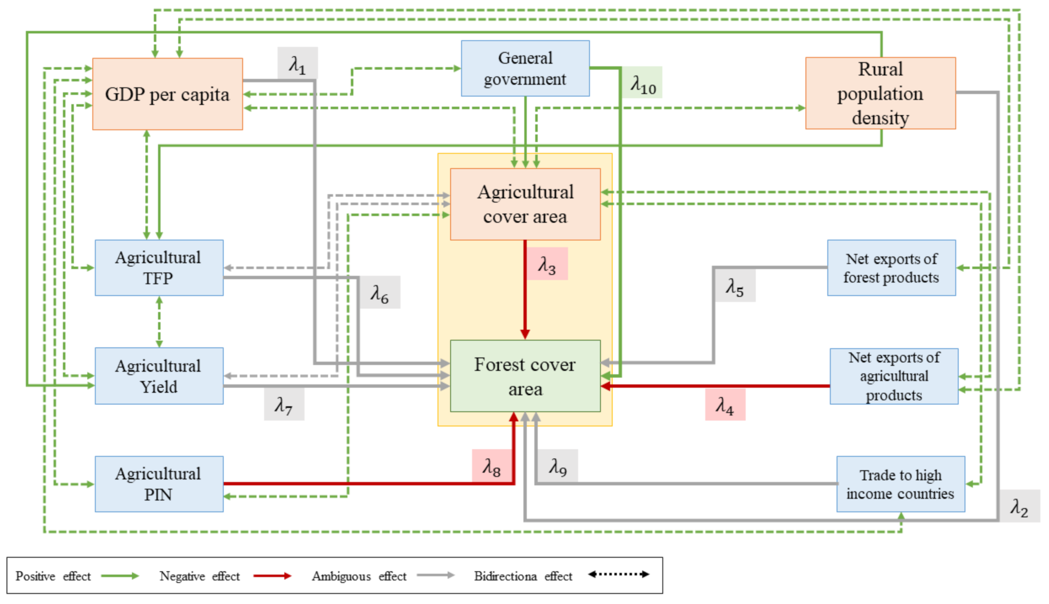
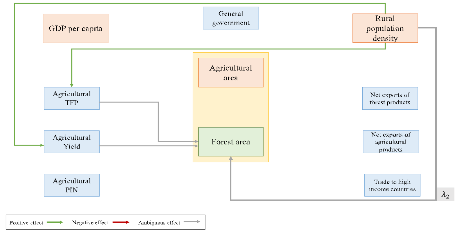
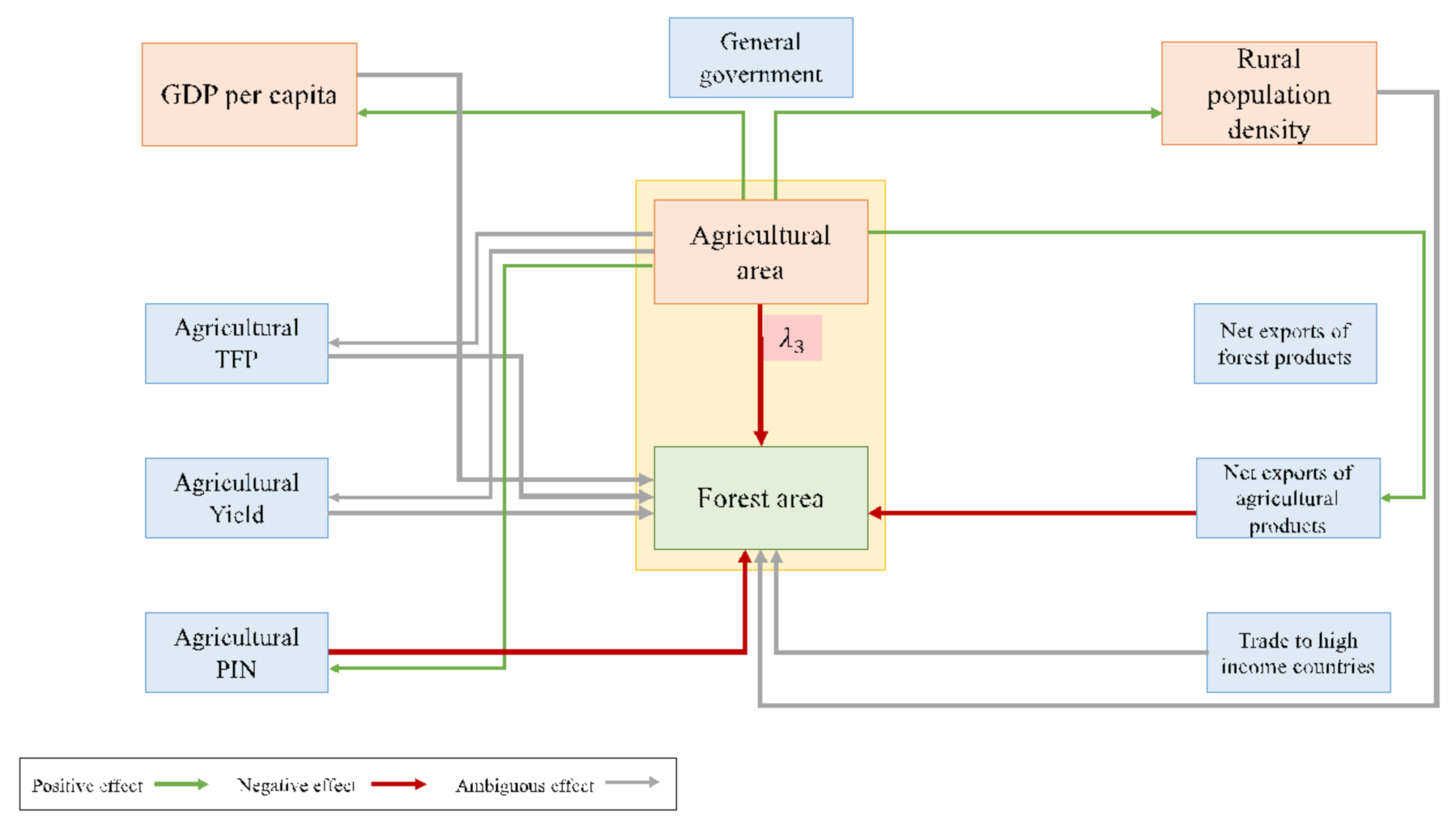
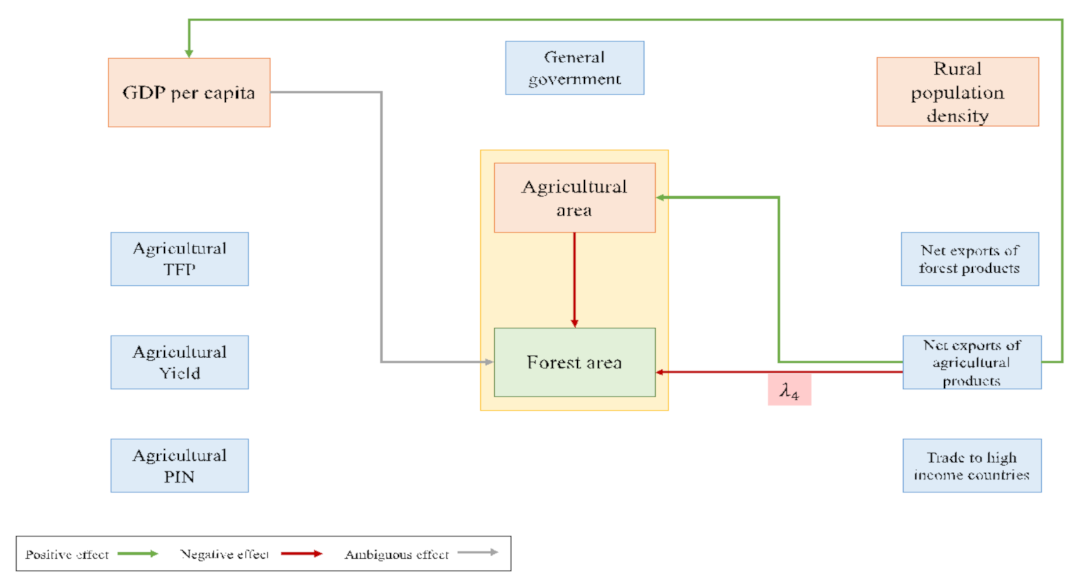
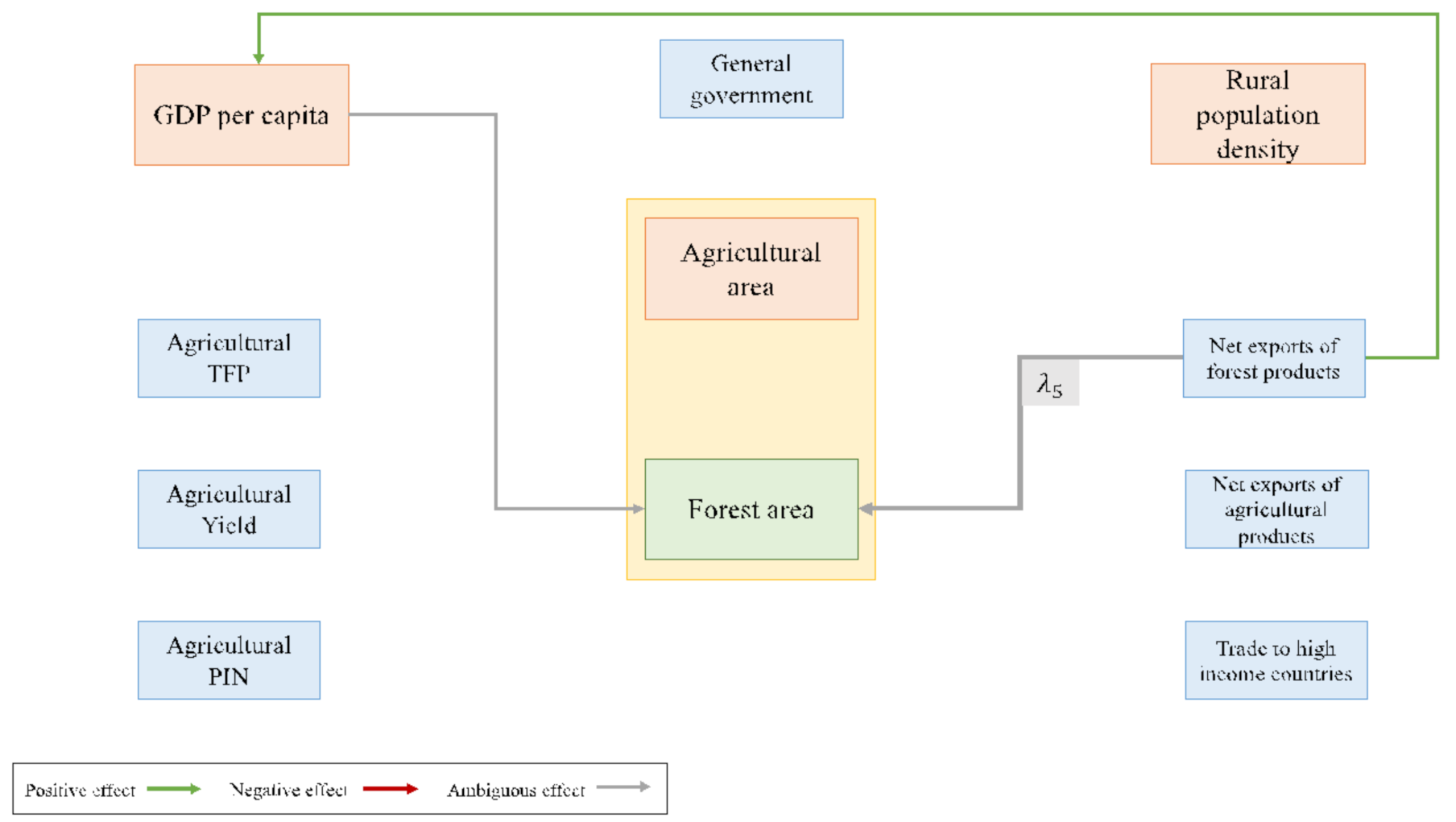
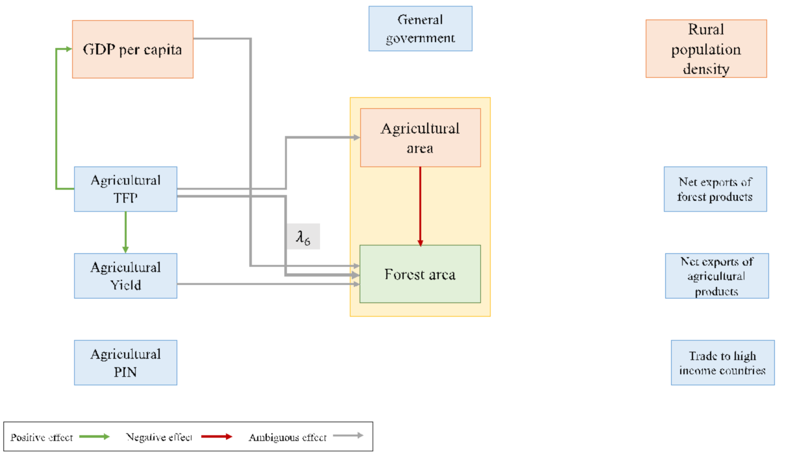
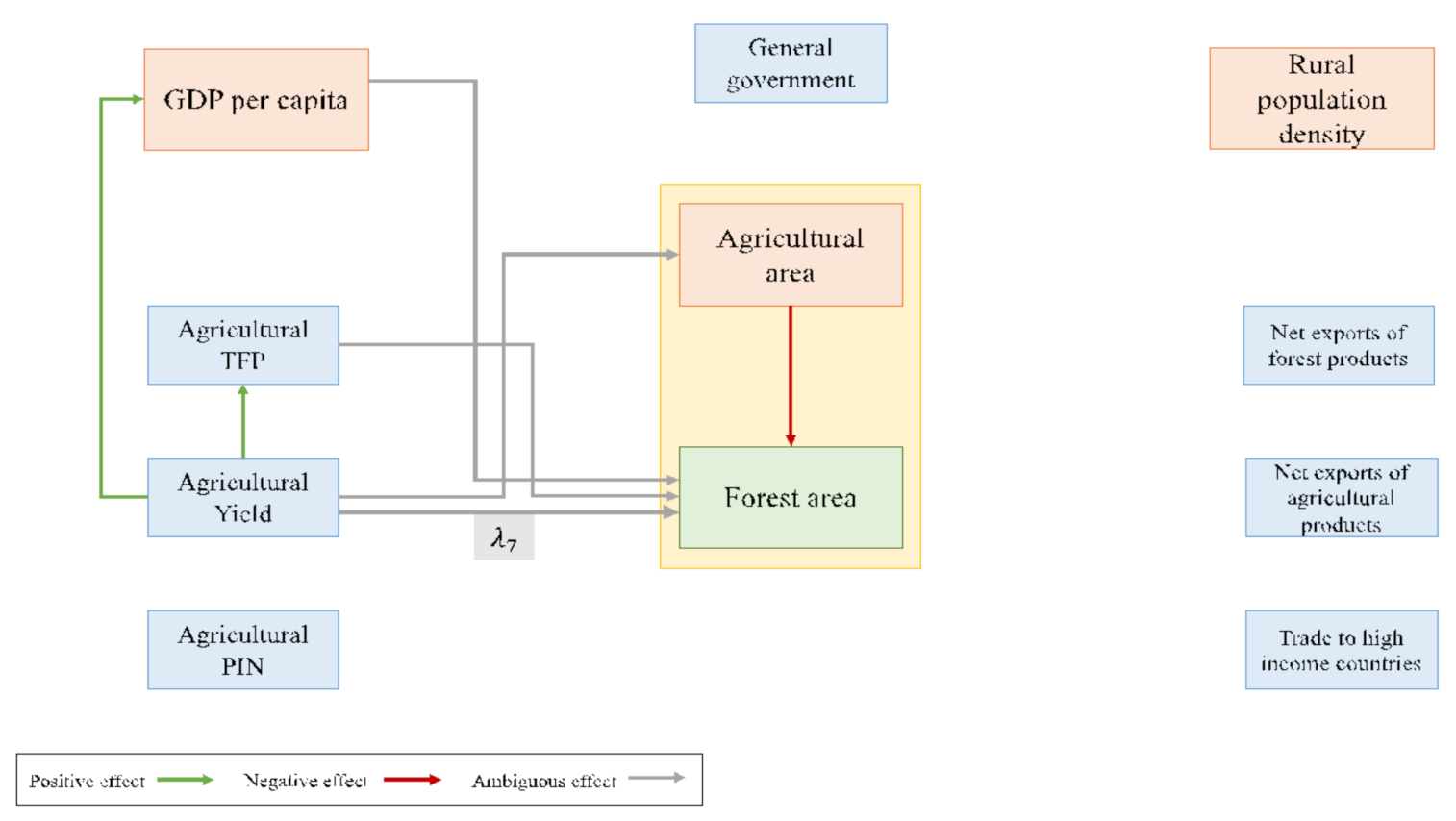
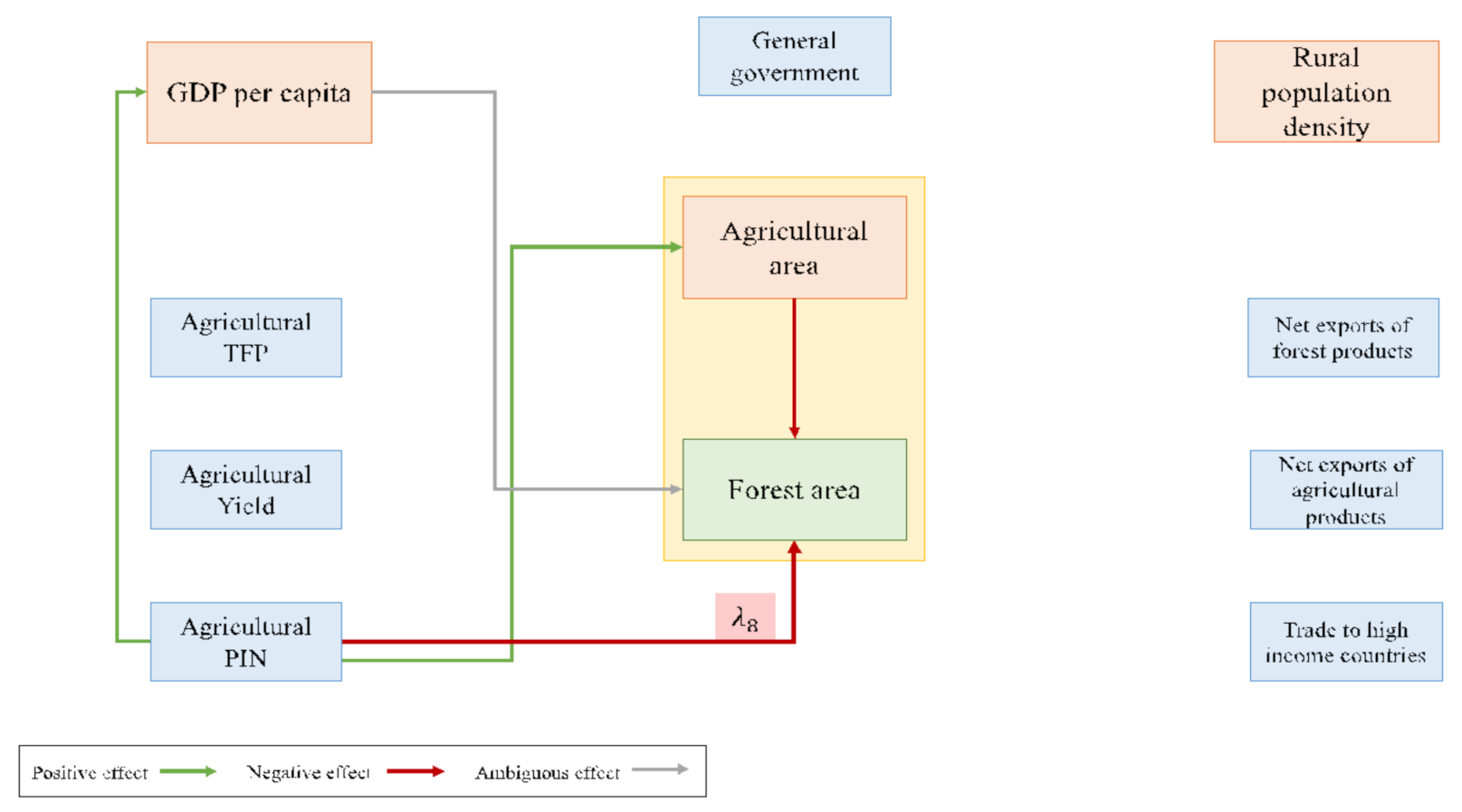
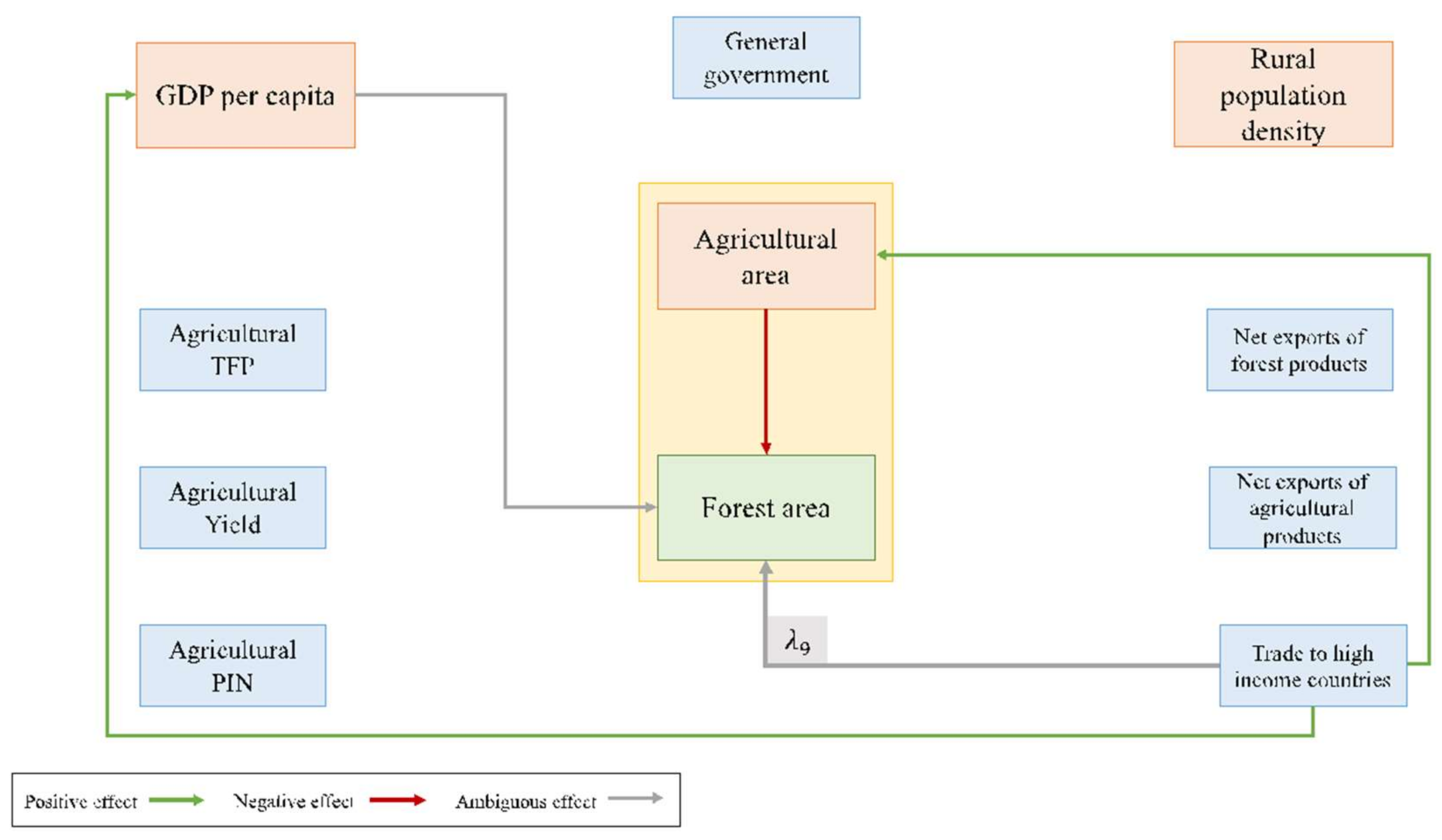
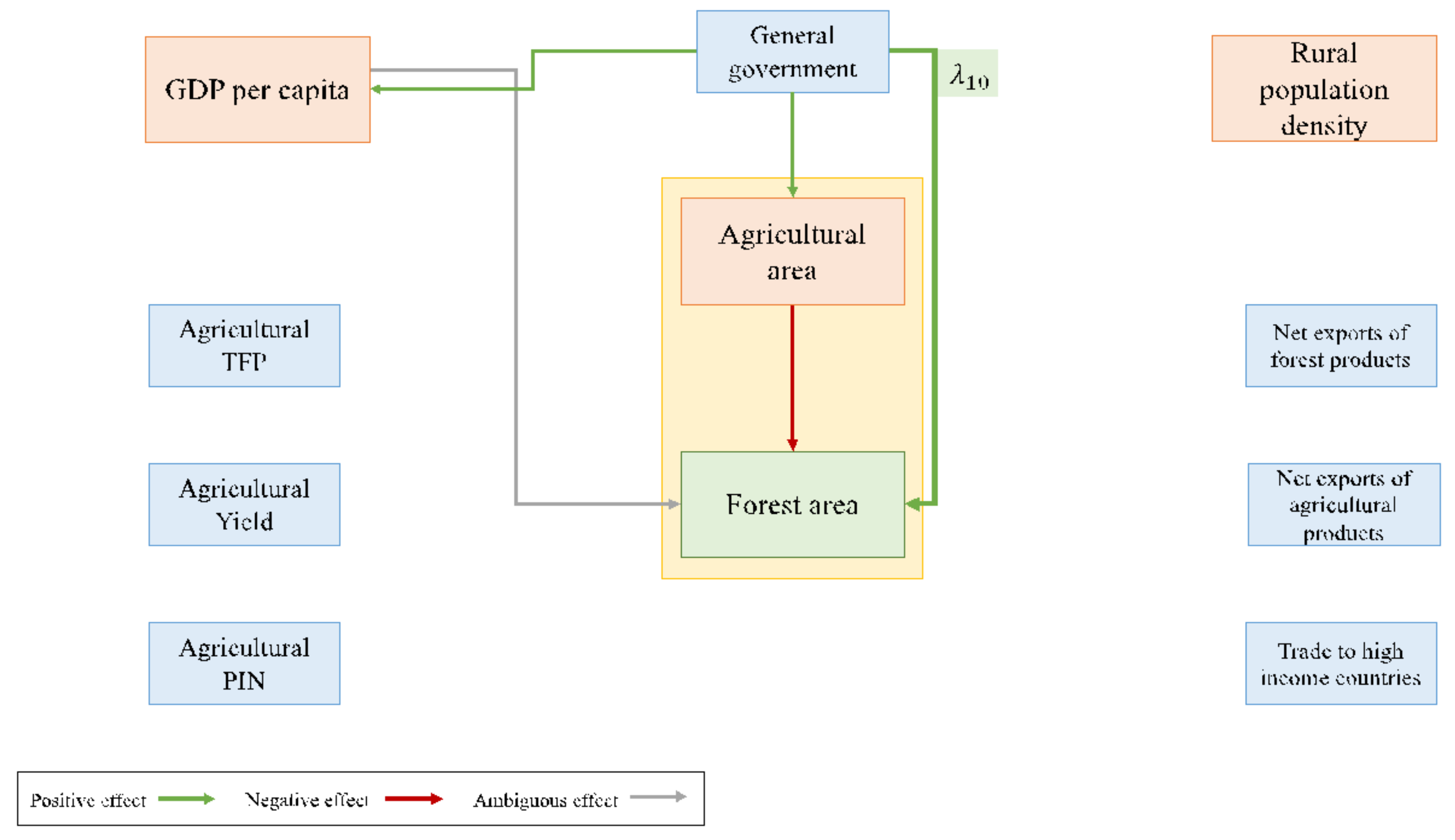
Taking into account these forest transition pathways and other environmental economics and environmental sociology theories, we have grouped our hypotheses in the following three groups: (1) the economic development path and the EKC; (2) the forest scarcity and forest policy pathways; (3) the globalization pathway together with the unequal ecological exchange theory. We formalized these hypotheses in a causal diagram (Figure 1), with their operationalization and expected signs explained in

Table 1. Hypotheses tested.

Hypothesis	Dependent Variable	Independent Variable (Level or First Differences)	Expected Signs
Hypothesis 1	Forest cover (% Land area)	GDP per capita	Negative
		GDP per capita2	Positive
	ΔForest cover (% Land area)	ΔGDP per capita	Negative
		ΔGDP per capita2	Positive
Hypothesis 2	ΔForest cover (% Land area)	Δagricultural employment	Negative
Hypothesis 3	ΔForest cover (% Land area)	ΔTFP	Positive
		Δagricultural yields	Positive
Hypothesis 4	ΔForest cover (% Land area)	Δ(Government quality/Forest t-1)	Positive
Hypothesis 5	ΔForest cover (% Land)	Error correction term	Negative
Hypothesis 6	ΔForest cover (% Land area)	ΔNet Exports of roundwoodΔNet Exports of agricultural products	Positive/Negative
Hypothesis 7	ΔForest cover (% Land area)	ΔTrade to high-income countries	Negative

.

This framework (Figure 1) is linked with the next section on the hypothesis tested and also with the methods section in the following way: The arrows containing a $\lambda$ coefficient represent the (direct) effects of those variables on forest, also captured by our econometric models (see coefficients in Equations (1) and (2)). The rest of the arrows represent the indirect effects of the variables on forest (captured by our procedure in Section 3.3). We attributed different expected signs to the $\lambda$ coefficients based on theoretical knowledge about each correspondent theory. We tested these hypotheses by comparing the sign of the coefficients in our model with the expected sign in Table 1.

2.1. Environmental Kuznets Curve and the “Economic Development” Pathway to Forest Transition

The EKC brought its name from Simon Kuznets who first explored the inverse U-shaped relationship between income per capita and income inequalities [20]. Later on, this was extended to the relationship between indicators of environmental degradation and economic growth [21,22]. Such EKC was applied to deforestation, by exploring a U-shaped relationship between rate of deforestation or forest cover and the income per capita [22,23]. The theory asserts that at low levels of development, the environmental degradation is limited to the subsistence economic activity on natural resources. During the course of economic growth, with increasing consumption, and thus agricultural expansion, income increases (in this paper, we use interchangeably the term income and gross domestic product (GDP)) are first positively related with deforestation (and thus a decrease in forest cover area). The shift to more industrialized economies spurred the impact of human activities on the environment with further exploitation of natural resources, such as primary forest products boosted by an increasing demand. However, after a certain level of economic development, further economic growth will be associated with a slowdown in deforestation till reaching a transition from forest losses to gains. Multiple mechanisms are hypothesized to allow this trajectory to happen—in particular, changes in economic and industrial structure with the advent of tertiary sectors, technological changes, and the creation of reforestation projects together with policy and societal changes and increased demand for environmental amenities [22,24]. The EKC literature for deforestation show conflictual results concerning the effective existence of a U-shaped relationship between deforestation and economic growth with a recent work which results seems to confirm a possible existence of it [10].

Similar to the EKC, the economic development path of forest transition theory links deforestation to the level of income. This path highlights the processes of urbanization and industrialization which drive labor force away from rural areas at the same time that agricultural intensification happens on the most suitable land. This switch from an agriculture-based economy to an industry or service-based one happens at a certain level of income per capital and capital stock which is different for each country. The sequence of events described by this path are the following: farm workers leave the land for better wages in non-farm sectors; the loss of laborers raises the salaries of the remaining workers and makes agriculture less profitable in areas that can hardly mechanize or with unfavorable agro-environmental conditions [18]. Thus, farmers in remote and less productive fields abandon their activity and these lands may potentially experience forest regrowth [1,4]. Improved markets and transport networks as well as infrastructures allow food’s redistribution from the most productive regions to the least productive ones, reinforcing the abandonment of agriculture in marginal regions and possibly their specialization in forestry. This leads to a U-shaped relationship between time and forest cover which is consistent with the EKC hypothesis applied to forest cover change assuming a continuous economic growth over time. Operationally, we thus used the quadratic form of GDP per capita as an aggregate measure of all structural changes coming from economic development and growth to test the general pattern posited in both theories. Yet, to move further, and because as identified above, multiple mechanisms are bundled in GDP measures, we included additional variables that allow us to test some of these main mechanisms. For this, we operationalized these narratives into the following testable hypotheses:

• Hypothesis 1: There is an inverted U-shaped relationship between deforestation and GDP per capita at an aggregate level. We test this hypothesis using the quadratic form of GDP per capita as an aggregate measure of economic growth.
• Hypothesis 2: A reduction in agricultural employment results in lower deforestation rates.
• Hypothesis 3: Increases in agricultural intensification, measured by either total factor productivity (TFP) and agricultural yields, lead to higher levels of forest area. In addition, we introduced an interaction term between agricultural intensification and GDP per capita on our model, hypothesizing that there may be a synergistic relation between the effects of these two dynamics on forest cover.

2.2. “Forest Scarcity” and “State Forest Policy” Forest Transition Pathways

Deforestation in a country, due to agricultural expansion, wood extraction or mining activities, may create a scarcity of forest products and a decrease in the ecosystem services that forest provides. In addition, this process could be reinforced by the increase in demand for wood products. Such perception of scarcity and degradation may, in turn, drive forest protection efforts, forestry intensification and tree-planting projects (“forest scarcity” pathway) including specific political responses (“state forest policy” pathway). Those feedback responses to low levels of forest cover could contribute to preserve the remaining forest and revert the decreasing trend of forest [1]. This has also been explored by others works such as [25]. Here we operationalized these feedback mechanisms through hypotheses 4 and 5:

• Hypothesis 4: Countries with higher government ability to draft and enforce stricter environmental and forest policies have a stronger effect of past decreasing forest area on present forest area. We operationalize this through an interaction between a proxy of environmental governance capacity and lagged forest cover. As a proxy for the government ability to draft and implement environmental legislation, we use an aggregate measure of the following indices: control of corruption, government effectiveness, regulatory quality, rule of law, voice and accountability (see variable “government quality” on

  Table A1. Definition and source of variables.

  Variable’s Name	Definition	Units	Source
  Forest (%)	Coefficient between: Forest cover (ha): the sum of tree-covered areas which includes any geographical area dominated by natural tree plants with a cover of 10 per cent or more. Areas planted with trees for afforestation purposes and forest plantations are included in this class and mangroves. And land area (ha): country area excluding area under inland waters and coastal waters.	%	Land Cover CCI Product User Guide Version 2.0 (2017). Reference: [14] (accessed on 15 January 2019)
  Agr land (%)	Coefficient between: (i) agricultural cover area defined as the sum of three CCI categories: herbaceous crops, wood crops, and grassland and (ii) land area.	%	Land Cover CCI Product User Guide Version 2.0 (2017). Reference: [14] (accessed on 15 January 2019)
  Rural pop density	Population living in rural areas over the land area of the country	Persons/ ha	The World Bank, Reference: [35] (accessed on 15 November 2018)
  GDP cap andGDP2 cap	Gross domestic product divided by midyear population.	Constant U.S. dollars (converted from domestic currencies using 2010 official exchange rates).	The World Bank, Reference: [35] (accessed on 15 November 2018)
  TFP	The ratio of an output index (total amount of crop and livestock output) to an index of land and non-land inputs (all land, labor, capital and material resources employed in farm production). To reduce potential index number bias in TFP growth estimates, cost shares are varied by decade whenever such information is available. For outputs, base year prices are fixed (the base period for output prices is 2004-06). Source: https://www.ers.usda.gov/data-products/international-agricultural-productivity/documentation-and-methods/	Unitless (ratio of outputs and inputs expressed in monetary terms). The change rate uses 1961 as the baseline year.	United States Department of Agriculture, Reference: [68] (accessed on 9 May 2019)
  Yield	Aggregate of all crops’ harvested production/harvested area for all crops.	Tonnes/ha.	FAOSTAT (FAO, 2018) Reference: [11] (accessed 15 June 2018)
  Agr (PIN)	Producer price index (2004–2016 = 100). It measures the average annual change over time in the selling prices received by farmers (prices at the farm gate or at the first point of sale).		FAOSTAT (FAO, 2018). Reference: [11] (accessed 15 June 2018)
  Agri empl (%)	Agricultural employment: Employment in agriculture (% of total employment) (modeled ILO estimate).	%	The World Bank, Reference: [35] (accessed on 15 November 2018)
  Agr prod net ex	Area of land embodied on exports of agricultural products (ha) minus imports agricultural products (ha).	ha	Own calculations using the data from [27].
  For prod net ex	Exports of roundwood (m3) minus imports of roundwood (m3)	m3	FAOSTAT (FAO, 2018) Reference: [11] (accessed 15 June 2018)
  Government quality	An average of the following four index: control of corruption, government effectiveness, regulatory quality, rule of law, voice and accountability.	Unitless	Worldwide Governance Indicators, www.govindicators.org, Reference: [69] (accessed on 15 June 2017)
  Trade high	Exports of agricultural products send to high-income countries divided by the total exports of agricultural products.	%	Own calculations using data from [27].
  Avg Temperature	Average temperature per year (computed from monthly data)	mm	The World Bank, Reference: [35] (accessed on 2 September 2019)
  Avg Rain	Average temperature per year (computed from monthly data)	Degrees Celsius	World Bank, Climate knowledge portal. Reference: [35] (accessed on 2 September 2019)

  on Appendix A).

Building on our statistical design using cointegration to investigate the long- and short-term dynamics, another way of testing this effect is through the error correction term (ECT) of the model. This term represents the forest’s speed of adjustment to the long-run forest equilibrium relationship with other variables (here GDP, agricultural area and rural population density). A larger, and more significant value of this parameter indicates that forest cover tends to adjust more rapidly to the long-term equilibrium relation between forest cover and these other variables. A larger value would thus suggest that changes in forest cover produce a relatively rapid feedback on land users’ decisions that then affects the forest cover itself. A smaller value would suggest that when GDP and other variables change, and with them the long-term equilibrium level of forest cover, the forest cover takes a longer time to adjust to this new equilibrium. However, it is not possible to specify how this response varies with either positive deviation of forest cover (abundance of forest) or negative deviation (forest scarcity).

• Hypothesis 5: There is a national feedback response from forest scarcity or forest abundance to the forest cover under the long equilibrium relationship. We test this hypothesis using the error correction term (ECT) variable: a significant ECT indicates that there is a feedback from forest abundance or scarcity on further forest cover levels, and thus the forest scarcity mechanism appears to hold, with larger values of ECT indicating stronger response.

2.3. “Globalization” Pathway of Forest Transition, and Ecologically Unequal Exchange Theory

These two theories point to trade with other countries as a mechanism that drives changes on national forest areas. With the increasing integration of the world via international trade, forest dynamics can no longer simply be explained by national dynamics such the ones explained on the previous forest transition paths [26]. Thus, the globalization pathway represents a modern version of the economic development pathway in which countries are integrate into global markets [19]. This integration influences the national-scale forest dynamics and also the national labor, capital, tourism and ideologies. For this work, we focus on the agricultural and roundwood international trade as a process that alters the national forest area. International trade could displace deforestation from countries that undergo a forest transition to regions with higher levels of forest area [19,26,27,28]. We tested the effect of net exports of agricultural products and roundwood on the exporter country through the following two hypotheses:

• Hypothesis 6a: National net exports of agricultural products have a negative effect on the national forest cover of the exporter country.
• Hypothesis 6b: National net exports of roundwood have an ambigous effect on national forest cover of the exporter country. On the one hand, roundwood exports may contribute to forest exploitation. On the other hand, these may incentivize tree plantation and improved management of forest resources [29].

The ecologically unequal exchange theory also identifies trade with other countries as a mechanism that drives changes on national forest areas. This theory points to trade between non-equivalent economically countries as a mechanism for cross-national disparities over access to environmental space [30]. As an effort to empirically test this theory, a recent work analized transfers of biophysical resources such as materials, energy, land and labor embodied on trade of comidities and services [31]. Other work from Jorgenson [32] applied this hypothesis to deforestation as follows: less-developed countries with higher levels of exports sent to more-developed countries experience greater rates of deforestation. We built our hypothesis on this work [32], and focused on agricultural products as the ones that are more likely to operate through this mechanism. Based on his work, we formulated the following hypothesis:

• Hypothesis 7: Exports of agricultural products to high-income countries have a negative effect on the national forest cover of the exporter country. We tested this hypothesis for low-, middle-, and high-income country groups, the latter being for consistency purposes as the theory is not supposed to apply to trade between high-income countries.

3. Materials and Methods

3.1. Data and Variables

We assembled an unbalanced panel dataset of country level variables covering the period 1992–2015. The dataset considered 111 countries, excluding those with less than 1 million hectares of forest cover in 2000. Those countries classified geographically are shown in

Table 2. Countries included in the analysis.

Africa	America	East and South Asia and Pacific	Europe and Central Asia
Angola	Argentina	Afghanistan	Austria
Benin	Belize	Australia	Azerbaijan
Burkina Faso	Bolivia	Bangladesh	Belarus
Cameroon	Brazil	Bhutan	Bosnia and Herzegovina
Central African Republic	Canada	Cambodia	Bulgaria
Congo, Dem. Rep.	Chile	China	Croatia
Congo, Rep.	Colombia	Fiji	Czech Republic
Cote d’Ivoire	Costa Rica	India	Estonia
Equatorial Guinea	Cuba	Indonesia	Finland
Ethiopia	Dominican Republic	Japan	France
Gabon	Ecuador	Korea, Rep.	Georgia
Ghana	El Salvador	Lao PDR	Germany
Guinea	Guatemala	Malaysia	Greece
Guinea-Bissau	Guyana	Myanmar	Hungary
Kenya	Honduras	Nepal	Iran, Islamic Rep.
Liberia	Mexico	New Zealand	Italy
Madagascar	Nicaragua	Pakistan	Kazakhstan
Malawi	Panama	Papua New Guinea	Kyrgyzstan
Morocco	Paraguay	Philippines	Latvia
Mozambique	Peru	Sri Lanka	Lithuania
Namibia	Suriname	Thailand	Norway
Niger	United States	Vietnam	Poland
Nigeria	Uruguay		Portugal
Senegal	Venezuela, RB		Romania
Sierra Leone			Russian Federation
South Africa			Slovak Republic
Sudan			Slovenia
Tanzania			Spain
Togo			Sweden
Uganda			Switzerland
Zambia			Turkey
Zimbabwe			Ukraine
			United Kingdom

but we used different classification for our analysis (Appendix B). Our data were retrieved from different sources. The dependent variable, forest cover, came from the CCI database [14]. The CCI database is a land cover dataset of the European Space Agency (ESA) derived from remote sensing. The category of forest tree coverage therein accounts for both natural forests as well as forest plantations. Many studies have used the Food and Agriculture Organization’s FRA data on forest area. Even though the CCI database cover shorter time span than the FRA’s data, we decided to use this dataset because of its focus on land cover (forested areas as measured by remote sensing with a spatial resolution of 300 m) instead of land use (land designated for forest use, as in the FAO data). We acknowledge that there are other relevant sources such as the widely used Global Forest Watch (GFW) dataset of Hansen et al. [33]. Nevertheless, we decided to rely on the CCI database for two main reasons: first, the time coverage, which is larger for CCI data, 1992–2015, compared to GFW, 2000–2019; second, GFW data consider only annual gross loss of forests, with less temporal details in measuring forest gains such as from natural regeneration or forest restoration. Because our analysis aims in assessing forest transition’s hypotheses, we needed a reliable source able to account for both forest losses and gains. Eventually, although some other land cover sources are characterized by a larger time span [8,34], several of our explanatory variables have shorter time span, which match with the CCI dataset. The list of all variables selected in our analysis are reported in Table A1 on Appendix A and, a reduced form of the table is presented below (

Table 3. Summary of variables.

Variable’s Name	Definition	Source
Forest (%)	Coefficient between: (i) forest cover (ha) (the sum of tree-covered areas and mangroves categories) and (ii) land area (ha) (country area excluding area under inland waters and coastal waters).	Land Cover CCI Product User Guide Version 2.0 (2017)
Agr land (%)	Coefficient between: (i) agricultural cover area (sum of herbaceous crops, wood crops, and grassland) and (ii) land area.	Land Cover CCI Product User Guide Version 2.0 (2017)
Rural pop density	Population living in rural areas over the land area of the country	World Bank
GDP cap; GDP2 cap	Gross domestic product divided by midyear population.	World Bank
TFP	The ratio of an output index (total amount of crop and livestock output) to an index of land and non-land inputs (all land, labor, capital and material resources employed in farm production). To reduce potential index number bias in TFP growth estimates, cost shares are varied by decade whenever such information is available. For outputs, base year prices are fixed (the base period for output prices is 2004-06). Source: https://www.ers.usda.gov/data-products/international-agricultural-productivity/documentation-and-methods/ (accessed on 9 May 2019)	United States Department of Agriculture
Yield	Aggregate of all crops’ harvested production/harvested area for all crops.	FAOSTAT (FAO, 2018)
Agr (PIN)	Producer price index (2004–2016=100). It measures the average annual change over time in the selling prices received by farmers (prices at the farm gate or at the first point of sale).	FAOSTAT (FAO, 2018)
Agri empl (%)	Agricultural employment: employment in agriculture (% of total employment) (modeled ILO estimate).	The World Bank
Agr prod net ex	Area of land embodied on exports of agricultural products (ha) minus imports agricultural products (ha).	Own calculations using the data from [27]
For prod net ex	Exports of roundwood (m3) minus imports of roundwood (m3)	FAOSTAT (FAO, 2018)
Government quality	An average of the following five indices: control of corruption, government effectiveness, regulatory quality, rule of law, voice and accountability.	Worldwide Governance Indicators
Trade high	Exports of agricultural products send to high-income countries divided by the total exports of agricultural products.	Own calculations using data from [27]
Avg temperature	Average temperature per year (computed from monthly data)	World Bank
Avg rain	Average temperature per year (computed from monthly data)	World Bank

).

We assumed cross-section independence in each group, and parameter homogeneity. We first performed the analyses separating the countries in three income groups following the World Bank’s clasification [35] (Appendix B). Thereafter, we classified countries according to their forest transition path following the classification suggested by Pendrill et al. [26] (Appendix B). These classifications were only made once for the whole analysis period (based on year 2018 for income groups, and on the classification directly retrieved from the work of Pendrill et al. [26], which is constructed over the period 2001–2015). Thus, when showing scatterplots for variables that change over time, the range of values of these different groups may partly overlap.

3.2. Time Series Properties of the Data

Many time series and panel techniques applied to test theories about forest cover and area assume that the series under investigation are stationary ( a stochastic time series whose probability distributions are stable over time; for a formal definition of stationary, see Wooldridge (p. 378) [36]) [7,37]. However, this assumption may lead to a misspecification as time series analyses are often affected by the problem of spurious regression [36,38]. This problem can appear when the dependent variable and at least one independent variable are non-stationary, i.e., their distribution (average and standard deviation) change over time. With non-stationary variables, the central limit theorem does not hold, and relations observed among these variables with ordinary least squares (OLS) regressions may be spurious, i.e., not reflecting a causal relationship among the two variables but being actually caused by a third variable, possibly time [36,39]. The notion of cointegration was developed by Granger [15] to address the spurious regression problem and make conclusions on the short- and long-run dynamics. If two time series are non-stationary individually but there exists a linear combination of them which is stationary, those variables are said to be cointegrated [40]. When such a cointegration relation can be identified, the regression is not spurious and describes the long-run equilibrium relationship between the variables, in which there must be causation in at least one direction [41]. The cointegration approach has been used in the energy domain [42,43] and by the land use and land cover change scientific community thanks to recent studies such the one from Rodríguez García et al. [13]. This study adopted the cointegration methodology to study dynamic interactions between cropland extent and intensity and it showed how this methodology can be successful on improving the understanding of land use dynamics.

We used Stata software for all analyses (version 15.1). We assessed the time series properties of our data by first testing the stationarity of our variables and assuming non-structural breaks. We used the Fisher unit root test to assess the stationary character of our variables, which allows for gaps in the panel series [44]. This test performs the Augmented Dickey–Fuller unit root tests on each panel to verify whether a variable has a unit root or, equivalently, that the variable follows a random walk, i.e., a process in which the dependent variable $y$ at time $t$ is obtained by starting at its previous value, $y_{t-1}$, and adding a zero mean random variable that is independent of $y_{t-1}$. This test performs a unit-root test on each panel (made of each variable) separately and combines the p-values to obtain an overall test [44]. We performed this test by income groups and clusters of forest transition phases by also including time trend and one lag for each test. The null hypothesis was that all panels contained a unit root, i.e., they were integrated of order 1, I(1) (the order of integration, denoted I(d), reports the minimum number of differences (d) required to obtain a stationary series, namely I(0)), or higher. The alternative was that at least one panel was stationary for each variable. We explored specifications with different lag structures up to four lags, but this introduced collinearity between the lag variables and the other variables of the model. Thus, we decided to use only one lag. When the variables were non-stationary, we continued by regressing them and testing for cointegration, i.e., for the stationarity of the error term of that regression. We tested for panel cointegration using the Pedroni’s test [45] and we choose to report the Modified Phillips–Perron t statistics for the sake of simplicity. Further results and other cointegration tests, namely [46,47], are available upon request. They show mixed results, but as a general pattern they suggest the possible presence of cointegration among the considered variables. The null hypothesis is ‘no cointegration’ against the alternative of ‘all panels are cointegrated.’ If the test rejected the null hypothesis of no cointegration, this indicated that the error term was stationary and that the variables were cointegrated.

3.3. Specification of the Dynamic Error Correction Model

Our time series were individually non-stationary and cointegrated, thus, they can be represented in the form of a dynamic error correction model [40]. We estimated this model by using the Engle and Granger two-step procedure [40]. First, we estimated the long-run cointegrating relationship (Equations (1) and (2). Second, we specified the short-run equations (Equations (3) and (4) by introducing in them the residuals of the long-run regressions (μ_i,), namely ECT. The ECT indicates the degree to which the equilibrium behavior drives short-run dynamics. The last period’s deviation from a long-run equilibrium influences its short-run dynamics. The ECT’s coefficient (${\lambda }_{15}$ in Equation (2)) should be statistically significant and comprised between -1 and 0 to adjust the variables towards the equilibrium keeping the long-run relationship intact, with a larger value indicating a more rapid adjustment [48]. This concept could be formalized through the idea that a proportion of the disequilibrium from one period is corrected in the next period [40]. The ECM also allows to obtain unbiased estimates of the short-run explanatory variables’ effects.

In these equations, i represents the cross-sectional component of the data and t the time series. We used a model with country fixed effects for both long- and short-run equations—controlling for the unobserved heterogeneity between countries such as climatic and other geographic conditions—and dummy variables for each year in the long-run equations to control for time fixed effects such as global inputs and outputs prices fluctuations or other uncontrolled weather conditions. Due to the lack of data at the national level we did not include timber prices in our analysis. Nonetheless, variations in timber prices on global markets are potentially captured by fixed effects. We also consider including the annual average temperature and rainfall as control variables on the long run to account for broader changes in environmental conditions, but they showed to be stationary in our time series, which is relatively short to capture remarkable changes in climate conditions, hence we decided not to include them in our long-run model. Further, we want to keep the long equation parsimonious and we assume that there is only one long term relationship for simplicity purposes. Thus, we only included gross domestic product per capita (hereafter as GDP), GDP², agricultural area, and rural population density on the long-run equation. We also estimated our long-run model with the inclusion of variables on: i) the net agricultural exports, and ii) the net forest product exports. However, these variables had a very small impact on forest dynamics (see Appendix C,

Table A2. Long run, income clusters, net agricultural exports as additional control variable.

Variables	(1)	(2)	(3)	(4)	(5)	(6)
	Low	Low	Middle	Middle	High	High
GDP cap (log)	0.199	−0.383	−0.061	−0.018	−0.56	0.023
GDP2 cap (log)	−0.014	0.03	0.004	0.001	0.033	−0.002
Rural pop (log)	0.009	−0.138	0.019	−0.035	−0.085	−0.066
Agr land (log)	−1.54		−0.243		−0.611
Agr prod net ex (ha)	0.000	0.000	0.000	0.000	0.000	0.000
Cons	−3.765	−0.282	−1.093	−0.985	0.484	−1.161
Observations	390	390	1216	1216	583	583
R-squared	0.562	0.053	0.18	0.028	0.411	0.107
Year dummies	Yes	Yes	Yes	Yes	Yes	Yes

Note: The long-run coefficient estimators are unbiased for the sample but not robust and thus cannot be directly used for statistical inference. For that reason, the significance is not indicated on the tables. Standard errors are in parentheses.

,

Table A3. Short run, income clusters, net agricultural exports as additional control variable.

Independent Variables	(1)	(2)	(3)	(4)	(5)	(6)
	Low	Low	Middle	Middle	High	High
LD.GDP cap (log)	0.127	0.222	−0.014	0.008	0.013	0.048
	(0.16)	(0.136)	(0.041)	(0.04)	(0.113)	(0.105)
LD.GDP2 cap (log)	−0.011	−0.018	0.001	0	0	−0.001
	(0.014)	(0.011)	(0.003)	(0.002)	(0.006)	(0.005)
LD.Rural pop (log)	0.081	0.124	−0.038	−0.044	0.018	0.005
	(0.199)	(0.167)	(0.031)	(0.03)	(0.03)	(0.027)
LD.Agr land (log)	−0.527 ***		−0.01		−0.113 **
	(0.113)		(0.013)		(0.049)
LD.Agr empl	0	−0.001	0	0	0	0
	(0.001)	(0.001)	(0)	(0)	(0)	(0)
D.Agr prod ex. (ln)	−0.006	−0.001	0	0	0.006	0.007
	(0.014)	(0.012)	(0.001)	(0.001)	(0.006)	(0.005)
LD.Agr prod net ex	0	0	0	0	0	0
	(0)	(0)	(0)	(0)	(0)	(0)
LD.For prod net ex	0	0	0	0	0	0
	(0)	(0)	(0)	(0)	(0)	(0)
LD.TFP	−0.719	3.189	−0.23	−0.603	0.488	0.31
	(2.975)	(2.52)	(0.505)	(0.498)	(0.741)	(0.694)
LD.Agr (PIN) (log)	−0.018	−0.004	0.007 **	0.007 **	0.002	0.001
	(0.018)	(0.015)	(0.003)	(0.003)	(0.006)	(0.006)
LD.Yield (log)	−0.006	−0.017	0	0	0.006	0.006 *
	(0.013)	(0.011)	(0.002)	(0.002)	(0.003)	(0.003)
LD.Trade high	0	−0.001	0 **	0 **	0	0 **
	(0.001)	(0.001)	(0)	(0)	(0)	(0)
LD.Government	−0.016	−0.01	−0.002	−0.005	−0.006	−0.007
	(0.021)	(0.017)	(0.003)	(0.003)	(0.008)	(0.008)
DL(Gov/L.For)	−0.006	−0.003	0.001 *	0	−0.002	−0.003
	(0.01)	(0.008)	(0)	(0)	(0.005)	(0.005)
LD.Temperature	−0.003	−0.003	−0.001 *	−0.001 *	0	0
	(0.003)	(0.002)	(0)	(0)	(0)	(0)
LD.Rainfall	0 **	0*	0	0	0	0
	(0)	(0)	(0)	(0)	(0)	(0)
L	−0.324 ***	−0.373 ***	−0.128 ***	−0.125 ***	−0.087 ***	−0.123 ***
	(0.04)	(0.025)	(0.011)	(0.01)	(0.018)	(0.015)
Cons	0.035 ***	0.018 ***	−0.003 ***	−0.003 ***	−0.007 ***	−0.007 ***
	(0.006)	(0.004)	(0)	(0)	(0.001)	(0.001)
Observations	226	226	771	771	364	364
R-squared	0.389	0.563	0.191	0.211	0.131	0.216

Standard errors are in parentheses, *** p < 0.01, ** p < 0.05, * p < 0.1.

,

Table A4. Long run, forest transition clusters, net agricultural exports as additional control variable.

Variables	(1)	(2)	(3)	(4)	(5)	(6)
	Early_&_Pre	Early_&_Pre	Late	Late	Post	Post
GDP cap (log)	−0.123	−0.102	0.069	0.082	0.048	0.000
GDP2 cap (log)	0.008	0.007	−0.003	−0.005	−0.004	−0.007
Rural pop (log)	−0.045	−0.04	0.123	0.052	0.017	−0.008
Agr land (log)	−0.243		−0.481		−0.502
Agr prod net ex (ha)	0	0	0	0	0	0
Cons	−0.592	−0.183	−2.14	−1.658	−1.769	−1.393
Observations	499	499	410	410	1280	1280
R-squared	0.277	0.177	0.424	0.096	0.178	0.027
Year dummies	Yes	Yes	Yes	Yes	Yes	Yes

Note: The long-run coefficient estimators are unbiased for the sample but not robust and thus cannot be directly used for statistical inference. For that reason, the significance is not indicated on the tables. Standard errors are in parentheses, *** p < 0.01, ** p < 0.05, * p < 0.1.

,

Table A5. Short run, forest transition clusters, net agricultural exports as additional control variable.

Independent Variables	(1)	(2)	(3)	(4)	(5)	(6)
	Early_&_Pre	Early_&_Pre	Late	Late	Post	Post
LD.GDP cap (log)	0.064	0.078	−0.084	−0.046	−0.132 ***	−0.144 ***
	(0.056)	(0.056)	(0.058)	(0.053)	(0.036)	(0.036)
LD.GDP2 cap (log)	−0.004	−0.004	0.005	0.002	0.008 ***	0.009 ***
	(0.004)	(0.004)	(0.004)	(0.003)	(0.002)	(0.002)
LD.Rural pop (log)	−0.158	−0.14	0.027	0.033	0.012	−0.007
	(0.166)	(0.165)	(0.047)	(0.042)	(0.026)	(0.026)
LD.Agr land (log)	−0.06 *		−0.04		−0.086 **
	(0.032)		(0.037)		(0.043)
LD.Agr empl	0	0	−0.001 **	−0.001	0	0
	(0.001)	(0.001)	(0)	(0)	(0)	(0)
D.Agr prod ex. (ln)	0.005	0.007	−0.001	0	0	0
	(0.009)	(0.009)	(0.006)	(0.005)	(0.001)	(0.001)
LD.Agr prod net ex	0	0	0	0	0	0
	(0)	(0)	(0)	(0)	(0)	(0)
LD.For prod net ex	0	0	0	0	0	0
	(0)	(0)	(0)	(0)	(0)	(0)
LD.TFP	1.667	0.068	−0.202	−0.059	0.034	−0.11
	(1.664)	(1.641)	(1.144)	(1.024)	(0.549)	(0.54)
LD.Agr (PIN) (log)	0.013	0.012	0.001	0.003	0.005	0.006
	(0.011)	(0.011)	(0.007)	(0.006)	(0.004)	(0.004)
LD.Yield (log)	−0.009	−0.011	−0.004	−0.004	0.001	0
	(0.01)	(0.01)	(0.005)	(0.004)	(0.002)	(0.002)
LD.Trade high	0	0	0	0	0 ***	0 ***
	(0)	(0)	(0)	(0)	(0)	(0)
LD.Government	−0.018	−0.026 **	0.004	0.003	−0.001	−0.003
	(0.011)	(0.011)	(0.009)	(0.008)	(0.004)	(0.004)
DL(Gov/L.For)	0.002 *	−0.001	0.001	0.001	0	−0.001
	(0.001)	(0.001)	(0.006)	(0.005)	(0.002)	(0.002)
LD.Temperature	−0.002	−0.001	−0.002 *	−0.002 *	0	0
	(0.002)	(0.002)	(0.001)	(0.001)	(0)	(0)
LD.Rainfall	0	0	0	0	0	0
	(0)	(0)	(0)	(0)	(0)	(0)
L	−0.314***	−0.302 ***	−0.201 ***	−0.206 ***	−0.171 ***	−0.165 ***
	(0.029)	(0.027)	(0.024)	(0.017)	(0.01)	(0.009)
Cons	−0.006**	−0.011 ***	0.021 ***	0.023 ***	−0.006 ***	−0.007 ***
	(0.003)	(0.003)	(0.003)	(0.002)	(0)	(0)
Observations	307	307	254	254	800	800
R-squared	0.336	0.338	0.304	0.433	0.3	0.32

*** p < 0.01, ** p < 0.05, * p < 0.1.

,

Table A6. Long run, income clusters, net agricultural exports and net exports of forests products as additional control variables.

Variables	(1)	(2)	(3)	(4)	(5)	(6)
	Low	Low	Middle	Middle	High	High
GDP cap (log)	0.171	−0.422	−0.063	−0.02	−0.495	0.061
GDP2 cap (log)	−0.012	0.034	0.005	0.001	0.028	−0.006
Rural pop (log)	−0.009	−0.136	0.019	−0.035	−0.068	−0.048
Agr land (log)	−1.51		−0.244		−0.579
Agr prod ex. (ln)	0.003	0.009	0	0	0.079	0.09
_cons	−3.698	−0.293	−1.084	−0.973	−0.813	−2.528
Observations	390	390	1216	1216	583	583
R-squared	0.562	0.06	0.179	0.026	0.524	0.253
Year dummies	Yes	Yes	Yes	Yes	Yes	Yes

*** p < 0.01, ** p < 0.05, * p < 0.1.

,

Table A7. Short run, income clusters, net agricultural exports and net exports of forests products as additional control variables.

Independent Variables	(1)	(2)	(3)	(4)	(5)	(6)
	Low	Low	Middle	Middle	High	High
LD.GDP cap (log)	0.122	0.237 *	−0.014	0.007	0.023	0.05
	(0.159)	(0.137)	(0.041)	(0.041)	(0.113)	(0.105)
LD.GDP2 cap (log)	−0.01	−0.02 *	0.001	0	−0.001	−0.002
	(0.013)	(0.011)	(0.003)	(0.002)	(0.006)	(0.005)
LD.Rural pop (log)	0.058	0.178	−0.04	−0.046	0.021	0.006
	(0.199)	(0.168)	(0.031)	(0.03)	(0.03)	(0.027)
LD.Agr land (log)	−0.523 ***		−0.01		−0.109 **
	(0.113)		(0.013)		(0.049)
LD.Agr empl	0	−0.001	0	0	0	0
	(0.001)	(0.001)	(0)	(0)	(0)	(0)
D.Agr prod ex. (ln)	−0.005	−0.004	0	0	0.008	0.01 *
	(0.014)	(0.012)	(0.001)	(0.001)	(0.006)	(0.005)
LD.Agr prod net ex	0	0	0	0	0	0
	(0)	(0)	(0)	(0)	(0)	(0)
LD.For prod net ex	0	0	0	0	0	0
	(0)	(0)	(0)	(0)	(0)	(0)
LD.TFP	−0.807	3.61	−0.233	−0.606	0.469	0.198
	(2.962)	(2.54)	(0.505)	(0.499)	(0.737)	(0.689)
LD.Agr (PIN) (log)	−0.018	−0.005	0.007 **	0.007 **	0	−0.002
	(0.018)	(0.015)	(0.003)	(0.003)	(0.006)	(0.006)
LD.Yield (log)	−0.006	−0.015	0	−0.001	0.006*	0.006 **
	(0.013)	(0.011)	(0.002)	(0.002)	(0.003)	(0.003)
LD.Trade high	0	−0.001	0 **	0 **	0	0 *
	(0.001)	(0.001)	(0)	(0)	(0)	(0)
LD.Government	−0.015	−0.012	−0.002	−0.005	−0.007	−0.01
	(0.021)	(0.018)	(0.003)	(0.003)	(0.008)	(0.008)
DL(Gov/L.For)	−0.005	−0.004	0.001 *	0	−0.003	−0.005
	(0.01)	(0.009)	(0)	(0)	(0.005)	(0.005)
LD.Temperature	−0.003	−0.003	−0.001 *	−0.001 *	0	0
	(0.003)	(0.002)	(0)	(0)	(0)	(0)
LD.Rainfall	0**	0*	0	0	0	0
	(0)	(0)	(0)	(0)	(0)	(0)
L	−0.326 ***	−0.372 ***	−0.127 ***	−0.125 ***	−0.104 ***	−0.142 ***
	(0.039)	(.025)	(0.011)	(0.01)	(0.021)	(0.016)
_cons	0.036 ***	0.015 ***	−0.003 ***	−0.003 ***	−0.009 ***	−0.009 ***
	(0.006)	(0.004)	(0)	(0)	(0.002)	(0.001)
Observations	226	226	771	771	364	364
R-squared	0.395	0.558	0.19	0.209	0.137	0.228

Standard errors are in parentheses, *** p < 0.01, ** p < 0.05, * p < 0.1.

,

Table A8. Long run, forest transition clusters, net agricultural exports and net exports of forests products as additional control variables.

Variables	(1)	(2)	(3)	(4)	(5)	(6)
	Early_&_Pre	Early_&_Pre	Late	Late	Post	Post
GDP cap (log)	0.005	0.004	0.066	0.079	0.049	0.084
GDP2 cap (log)	0	0	−0.003	−0.005	−0.004	−0.007
Rural pop (log)	−0.061	−0.061	0.126	0.059	0.017	−0.008
Agr land (log)	−0.279		−0.489		−0.502
Agr prod ex. (ln)	−0.078	−0.049	0.003	0.005	0.001	0.001
_cons	−0.066	0.069	−2.176	−1.693	−1.778	−1.401
Observations	499	499	410	410	1280	1280
R-squared	0.319	0.193	0.423	0.073	0.178	0.027
Year dummies	Yes	Yes	Yes	Yes	Yes	Yes

Standard errors are in parentheses, *** p < 0.01, ** p < 0.05, * p < 0.1.

,

Table A9. Short run, forest transition clusters, net agricultural exports and net exports of forests products as additional control variables.

Independent Variables	(1)	(2)	(3)	(4)	(5)	(6)
	Early_&_Pre	Early_&_Pre	Late	Late	Post	Post
LD.GDP cap (log)	0.026	0.056	−0.081	−0.044	−0.132 ***	−0.144 ***
	(0.056)	(0.056)	(0.058)	(0.053)	(0.036)	(0.036)
LD.GDP2 cap (log)	−0.001	−0.003	0.004	0.002	0.008 ***	0.009 ***
	(0.004)	(0.004)	(0.004)	(0.003)	(0.002)	(0.002)
LD.Rural pop (log)	−0.013	−0.044	0.016	0.013	0.012	−0.007
	(0.166)	(0.165)	(0.047)	(0.043)	(0.026)	(0.025)
LD.Agr land (log)	−0.061 *		−0.041		−0.086 **
	(0.032)		(0.037)		(0.043)
LD.Agr empl	0	0	−0.001 **	0	0	0
	(0.001)	(0.001)	(0)	(0)	(0)	(0)
D.Agr prod ex. (ln)	−0.005	0.001	0	0.002	0	0
	(0.009)	(0.009)	(0.006)	(0.005)	(0.001)	(0.001)
LD.Agr prod net ex	0	0	0	0	0	0
	(0)	(0)	(0)	(0)	(0)	(0)
LD.For prod net ex	0	0	0	0	0	0
	(0)	(0)	(0)	(0)	(0)	(0)
LD.TFP	2.084	0.232	−0.179	0.016	0.037	−0.106
	(1.68)	(1.646)	(1.143)	(1.033)	(0.549)	(0.539)
LD.Agr (PIN) (log)	0.019 *	0.015	0.001	0.004	0.005	0.006
	(0.012)	(0.011)	(0.007)	(0.006)	(0.004)	(0.004)
LD.Yield (log)	−0.014	−0.013	−0.004	−0.005	0.001	0
	(0.01)	(0.01)	(0.005)	(0.004)	(0.002)	(0.002)
LD.Trade high	0	0	0	0	0***	0 ***
	(0)	(0)	(0)	(0)	(0)	(0)
LD.Government	−0.012	−0.023 **	0.004	0.004	−0.001	−0.003
	(0.011)	(0.011)	(0.009)	(0.008)	(0.004)	(0.004)
DL(Gov/L.For)	0.002 *	−0.001	0.001	0.002	0	−0.001
	(0.001)	(0.001)	(0.006)	(0.005)	(0.002)	(0.002)
LD.Temperature	−0.002	−0.001	−0.002 **	−0.002 *	0	0
	(0.002)	(0.002)	(0.001)	(0.001)	(0)	(0)
LD.Rainfall	0	0	0	0	0	0
	(0)	(0)	(0)	(0)	(0)	(0)
L	−0.318 ***	−0.304 ***	−0.2 ***	−0.195 ***	−0.171 ***	−0.165 ***
	(0.03)	(0.027)	(0.023)	(0.017)	(.01)	(0.009)
_cons	−0.006 **	−0.011 ***	0.021 ***	0.022 ***	−0.006 ***	−0.007 ***
	(0.003)	(0.003)	(0.003)	(0.002)	(0)	(0)
Observations	307	307	254	254	800	800
R-squared	0.328	0.335	0.305	0.422	0.301	0.32

Standard errors are in parentheses, *** p < 0.01, ** p < 0.05, * p < 0.1.

). Therefore, we decided to keep the long-run model without these additional variables. In order to characterize indirect impacts, we specified two long-run equations, with and without the agricultural area (Equations (1) and (3). Changes in agricultural area are expected to be a key mediator through which other underlying causes such as GDP and rural population density affect forest cover (Figure 1). Thus, using models with and without agricultural area allowed us to identify the net effects of these underlying variables as well as to assess how much of this effect is mediated by agricultural area changes. The presence of cointegration is sufficient to prove the existence of at least one non-spurious long-run causal relationship between the variables. Yet, the estimated coefficients represent the net effect of a system of relationships and statistical infer-ence is not straightforward (see Appendix D for further explanation). Thus, we use the long run estimators only for our sample.

In the short-run models, we used first differences and we lag the variables by one period to avoid endogeneity between the variables (Equations (3) and (4). As explained above, we limited the number of variables that we included in the long-run regression for the error correction model. However, there is no corresponding limit for the short-run model; thus, we included additional variables to test our hypotheses as long as other control variables. We performed different robustness checks by excluding the variables agricultural production price index or, GDP² from our short-run model. For both variables, their absence did not influence much the results; however, we opted for maintaining them in the presented results as they constitute important control variables. We also tested the interaction terms of GDP with TFP and GDP with agricultural yield in the short run. However, we did not include those interaction terms in the final results as they were not significant, and their inclusion would have reduced the degree of freedom or our models.

3.3.1. Long-Run Model Specifications (with and without Agricultural Cover Area)

$$\begin{array}{ll}{\mathit{LogForest}}_{i,t}={\propto }_{1i}& +{\beta }_1{\mathit{LogGDPcap}}_{i,t}+{\beta }_2{\mathit{LogGDPcap}}_{i,t}^2+{\beta }_3{\mathit{logAgri}}_{i,t}+{\beta }_4{\mathit{LogRuralPopDensity}}_{i,t}\\ & +{\beta }_5{\mathit{timedummy}}_t+{\mu }_{i,t}\end{array}$$

(1)

$${\mathit{LogForest}}_{i,t}={\propto }_{1i}+{\beta }_1{\mathit{LogGDPcap}}_{i,t}+{\beta }_2{\mathit{LogGDPcap}}_{i,t}^2+{\beta }_3{\mathit{LogRuralPopDensity}}_{i,t}+{\beta }_4{\mathit{timedummy}}_t+{\mu }_{i,t}$$

(2)

For all equations:

$$iϵ\left\{1,2,\dots .,N\right\},tϵ\left\{1,2,\dots .,T_i\right\},{\mu }_{i,t}\left(0,{\sigma }_{\mu }^2\right)$$

It has to be noted that these long-run coefficients are superconsistent, i.e., the distribution of the estimated coefficients converges to the real value as the sample size tends to infinity [36]. However, their standard errors are large and unreliable, and thus not robust, so statistical inference is not straightforward [3,49]. Thus, we have only used those estimates for our sample without performing statistical inference (see Appendix C for futher explanation).

3.3.2. Short-Run Model Specifications (with and without Agricultural Cover Area)

$$\begin{array}{ll}\Delta {\mathit{LogForest}}_{i,t}=& {\lambda }_1\Delta {\mathit{LogGDPcap}}_{i,t-1}+{\lambda }_2\Delta {\mathit{LogGDPcap}}_{i,t-1}^2+{\lambda }_3\Delta {\mathit{LogRuralPopDensity}}_{i,t-1}+{\lambda }_4\Delta {\mathit{LogAgri}}_{i,t-1}\\ & +{\lambda }_5\Delta {\mathit{NetExportsAgri}}_{i,t-1}+{\lambda }_6\Delta {\mathit{NetExportForest}}_{i,t-1}+{\lambda }_7\Delta {\mathit{TFP}}_{i,t-1}\\ & +{\lambda }_8\Delta {\mathit{LogYield}}_{i,t-1}+{\lambda }_9\Delta \mathit{LogAgri}{\left(\mathit{PIN}\right)}_{i,t-1}+{\lambda }_{10}\Delta {\mathit{TradeHigh}}_{i,t-1}+{\lambda }_{11}\Delta {\mathit{Goverment}}_{i,t-1}\\ & +{\lambda }_{12}\Delta \mathit{AgriEmployment}+{\lambda }_{13}\Delta \mathit{Temperature}\left(\mathit{avg}\right)+{\lambda }_{14}\Delta \mathit{Rainfall}\left(\mathit{avg}\right)+{\lambda }_{15}{\mu }_{i,t-1}+{\epsilon }_{i,t}\end{array}$$

(3)

$$\begin{array}{ll}\Delta {\mathit{LogForest}}_{i,t}=& {\lambda }_1\Delta {\mathit{LogGDPcap}}_{i,t-1}+{\lambda }_2\Delta {\mathit{LogGDPcap}}_{i,t-1}^2+{\lambda }_3\Delta {\mathit{LogRuralPopDensity}}_{i,t-1}\\ & +{\lambda }_4\Delta {\mathit{NetExportsAgri}}_{i,t-1}+{\lambda }_5\Delta {\mathit{NetExportForest}}_{i,t-1}+{\lambda }_6\Delta {\mathit{TFP}}_{i,t-1}\\ & +{\lambda }_7\Delta {\mathit{LogYield}}_{i,t-1}+{\lambda }_8\Delta \mathit{LogAgri}{\left(\mathit{PIN}\right)}_{i,t-1}+{\lambda }_9\Delta {\mathit{TradeHigh}}_{i,t-1}+{\lambda }_{10}\Delta {\mathit{Goverment}}_{i,t-1}\\ & +{\lambda }_{11}\Delta \mathit{AgriEmployment}+{\lambda }_{12}\Delta \mathit{Temperature}\left(\mathit{avg}\right)+{\lambda }_{13}\Delta \mathit{Rainfall}\left(\mathit{avg}\right)+{\lambda }_{14}{\mu }_{i,t-1}+{\epsilon }_{i,t}\end{array}$$

(4)

3.4. Assessment of Indirect Effects in the Short Run

Based on our theoretical causal framework (Figure 1), we further explored the direct and indirect short-run relations between the variables. The short-run coefficients in Equation (2) capture the direct effect of each independent variable on the dependent variable, as well as the indirect effects through variables that are not included in the model. However, the effect of a given variable $X_1$ that is mediated by other variables present in the model is not captured in the coefficient of this variable $X_1$. Those effects refer to the correlation between independent variables, also known as multicollinearity. Our goal is not to correct for multicollinearity, as it does not bring any bias to our estimators unless it is perfect collinearity [36], but to assess the indirect effects between independent variables. If we take into account these indirect effects, the matrix information of the regression would not change but the significance and the absolute size of the regression may change [50]. To assess the influence of these indirect effects of our independent variables on the outcome variable for the short-run analysis, we carried out two approaches. In the first one, we performed our model without the agricultural area variable, as this variable is a key mediator for many other drivers of forest cover change. In the second approach, instead, we used simple algebra on the coefficients obtained by the least squared method. In this procedure, we decided to exclude the variables of average temperature and average rainfall; we assumed that those variables impact all other independent variables and we used them essentially as control variables, not as variables that are part of our focus on the causal framework (Figure 1). This simple way of assessing indirect effects does not bring any bias.

The second approach to assess the influence of indirect effect is characterized by the following four steps (see Appendix E for further exploration of this method, Figure A2, Figure A3, Figure A4, Figure A5, Figure A6, Figure A7, Figure A8, Figure A9, Figure A10, Figure A11):

• Step 1. Short-run regression: direct effects.

This step corresponds to Equation (3) in the previous section but excluding the variables annual average rain and temperature as well as the interaction term between government quality and forest, due to simplicity purposes. From this equation, we obtained the direct effects (${\lambda }_1$ to ${\lambda }_{15}$) of each independent variable on the dependent variable.

$$\begin{array}{ll}\Delta {\mathit{LogForest}}_{i,t}=& {\lambda }_1\Delta {\mathit{LogGDPcap}}_{i,t-1}+{\lambda }_2\Delta {\mathit{LogGDPcap}}_{i,t-1}^2+{\lambda }_3\Delta {\mathit{LogRuralPopDensity}}_{i,t-1}+{\lambda }_4\Delta {\mathit{LogAgri}}_{i,t-1}\\ & +{\lambda }_5\Delta {\mathit{NetExportsAgri}}_{i,t-1}+{\lambda }_6\Delta {\mathit{NetExportForest}}_{i,t-1}+{\lambda }_7\Delta {\mathit{TFP}}_{i,t-1}\\ & +{\lambda }_8\Delta {\mathit{LogYield}}_{i,t-1}+{\lambda }_9\Delta \mathit{LogAgri}{\left(\mathit{PIN}\right)}_{i,t-1}+{\lambda }_{10}\Delta {\mathit{TradeHigh}}_{i,t-1}+{\lambda }_{11}\Delta {\mathit{Goverment}}_{i,t-1}\\ & +{\lambda }_{12}\Delta \mathit{AgriEmployment}+{\lambda }_{13}\Delta \mathit{Temperature}\left(\mathit{avg}\right)+{\lambda }_{14}\Delta \mathit{Rainfall}\left(\mathit{avg}\right)+{\lambda }_{15}{\mu }_{i,t-1}+{\epsilon }_{i,t}\end{array}$$

(5)

• Step 2. Orthogonalization of independent variables: indirect effects.

The orthogonalization of variables is a transformation by which variables that were correlated become perfectly uncorrelated, i.e., orthogonal (here we use orthogonal and non-correlated as synonyms; see [51] for a formal definition of orthogonality). This transformation can be achieved without altering the disturbance term of the regression model in which the variables are embedded. The transformation we made consisted on breaking our multivariate short-run model (Equation (3)) into simpler bivariate models. We estimated a set of auxiliary regressions for each targeted independent variable (henceforth named as “$x_1$”). We built one auxiliary regression for each variable to which $x_1$ has an indirect impact to, and this $x_1$ was introduced as a regressor in each of these auxiliary regressions. Afterwards, we estimated the residuals of these auxiliary regressions. They capture the part of the dependent variable’s auxiliary regression that is orthogonal to, or thus not explained, by the variable $x_1$. If those residuals are equal to zero, there is perfect multicollinearity between the variable $x_1$ and the auxiliary variable—in that case, we would originally not have included both variables in our model. In the example below, we apply those steps for $x_1$ being equal to the variable ${\mathit{NetExportsAgri}}_{i,t}$.

Auxiliary Equation:

$$\Delta {\mathrm{LogGDP}}_{i,t-1}={\gamma }_1\Delta {\mathit{NetExportsAgri}}_{i,t-1}+{\mathit{residual}}_{\mathit{gdp}}$$

(6)

Auxiliary Equation:

$$\Delta {\mathit{LogGDPcap}}_{i,t-1}^2={\gamma }_2\Delta {\mathit{NetExportsAgri}}_{i,t-1}+{\mathit{residual}}_{\mathit{gdp}2}$$

(7)

Auxiliary Equation:

$$\Delta {\mathit{LogAgri}}_{i,t-1}={\gamma }_3\Delta {\mathit{NetExportsAgri}}_{i,t-1}+{\mathit{residual}}_{\mathrm{Agri}}$$

(8)

• Step 3. Netting out indirect and direct effects: total effect.

Thirdly, we netted out the direct and indirect effects in order to estimate the total or net effect of each targeted variable ($x_1$). For that, we ran a modified version of Step 1′s regression which consists in replacing the corresponding original variables on Equation (3) ($\Delta LogAgr{i}_i$ and $\Delta LogGDP,\Delta LogGD{P}^2{}_i$ in our example) with the corresponding residuals obtained from Step 2′s auxiliary regressions ($residua{l}_{Agri}$, $residua{l}_{gdp},residua{l}_{gdp2}$). The total effect of variable $x_1$ on forest cover area is the sum of two different effects: the direct effect (${\lambda }_5$ on Step 1) and the indirect effects of this variable through the auxiliary variables (${{\lambda }^{\prime }}_1{\gamma }_1+{{\lambda }^{\prime }}_2{\gamma }_2+{{\lambda }^{\prime }}_4{\gamma }_3$). We obtained one modified regression for each variable of focus. Those modified regressions are linear combinations of Equation (3).

$$\begin{array}{ll}\Delta {\mathit{LogForest}}_{i,t}=& {{\lambda }^{\prime }}_1\Delta {\mathit{residual}}_{\mathit{gdp}}{}_{i,t-1}+{{\lambda }^{\prime }}_2\Delta {\mathit{residual}}_{\mathit{gdp}2}{}_{i,t-1}+{{\lambda }^{\prime }}_3\Delta {\mathit{LogRuralPopDensity}}_{i,t-1}\\ & +{{\lambda }^{\prime }}_4\Delta {\mathit{residual}}_{{\mathit{agri}}_{i,t-1}}+({{\lambda }^{\prime }}_5+{{\lambda }^{\prime }}_1{\gamma }_1+{{\lambda }^{\prime }}_2{\gamma }_2+{{\lambda }^{\prime }}_4{\gamma }_3)\Delta {\mathit{NetExportsAgri}}_{i,t-1}\\ & +{{\lambda }^{\prime }}_6\Delta {\mathit{NetExportForest}}_{i,t-1}+{{\lambda }^{\prime }}_7\Delta {\mathit{TFP}}_{i,t-1}+{{\lambda }^{\prime }}_8\Delta {\mathit{LogYield}}_{i,t-1}+{{\lambda }^{\prime }}_9\Delta \mathit{LogAgri}{\left(\mathit{PIN}\right)}_{i,t-1}\\ & +{{\lambda }^{\prime }}_{10}\Delta {\mathit{TradeHigh}}_{i,t-1}+{{\lambda }^{\prime }}_{11}\Delta {\mathit{Goverment}}_{i,t-1}+{\lambda }_{12}\Delta \mathit{AgriEmployment}\\ & +{{\lambda }^{\prime }}_{13}\mathit{Temperature}\left(\mathit{avg}\right)+{{\lambda }^{\prime }}_{14}\mathit{Rainfall}\left(\mathit{avg}\right)+{{\lambda }^{\prime }}_{15}{\mu }_{i,t-1}^{}+u_{i,t}\end{array}$$

(9)

• Step 4. Total vs. direct effect.

Eventually, we compared the direct effect (${\lambda }_5$) and total effect $\left({{\lambda }^{\prime }}_5+{{\lambda }^{\prime }}_1{\gamma }_1+{{\lambda }^{\prime }}_2{\gamma }_2+{{\lambda }^{\prime }}_4{\gamma }_3\right)$ of the independent variable of interest—net exports of agricultural products in this example—and discussed the relative differences.

4. Results

4.1. Panel Unit Root Test and Cointegration Test Results

The stationarity tests of the variables forest cover, GDP, GDP², agricultural area, and rural population density for income and forest transition clusters, respectively (Table 2 and Table 3), showed that the variables are non-stationary of order 1, I(1), for GDP, GDP², and agricultural area. Concerning rural population density, the results suggest an I(0) variable but the visual inspection of the data suggests that it can be considered as a non-stationary variable (Appendix F, Figure A12, Figure A13, Figure A14). Furthermore, other panel data studies which used population as control variable in their analysis conclude I(1) as a result [52,53]. For the sake of simplicity, only one test (inverse Chi-squared) was reported (additional results are available upon request). Assuming that all our variables are I(1), we tested the presence for panel cointegration through the Pedroni test [45]. The results indicated the presence of cointegration among the considered variables for income and for forest transition clusters, respectively (Appendix G).

4.2. Results by Income Groups

In line with the results from the cointegration test, we found a long-run equilibrium relationship between the variables forest cover, GDP, GDP², agricultural area, and rural population density (

Table 4. Long-run equations, income clusters.

Variables	(1)	(2)	(3)	(4)	(5)	(6)
	Low	Low	Middle	Middle	High	High
GDP cap (log)	0.168	−0.357	−0.071	−0.030	−0.406	0.072
GDP2 cap (log)	−0.013	0.029	0.005	0.002	0.024	−0.004
Rural pop (log)	−0.025	−0.108	0.020	−0.031	−0.073	−0.072
Agr land (log)	−1.357		−0.258		−0.515
Const.	−3.461	−0.352	−1.081	−0.937	−0.014	−1.474
Obs.	470	470	1455	1455	703	703
R-squared	0.489	0.042	0.187	0.027	0.360	0.126
Year dummies	Yes	Yes	Yes	Yes	Yes	Yes

Note: The estimators are unbiased for the sample but not robust and thus cannot be directly used for statistical inference. Therefore, we interpreted those results only for our sample, which it is the reason why standard errors are not reported.

and

Table 5. Short-run equations, income clusters.

Independent Variables	(1)	(2)	(3)	(4)	(5)	(6)
	Low	Low	Middle	Middle	High	High
LD.GDP cap (log)	0.097	0.244 *	−0.009	0.013	0.004	0.043
	(0.145)	(0.126)	(0.039)	(0.039)	(0.106)	(0.101)
LD.GDP2 cap (log)	−0.008	−0.020 *	0.001	−0.001	0.000	−0.001
	(0.012)	(0.011)	(0.002)	(0.002)	(0.005)	(0.005)
LD.Rural pop (log)	0.043	0.181	−0.040	−0.048 *	0.007	0.001
	(0.174)	(0.149)	(0.030)	(0.029)	(0.027)	(0.025)
LD.Agr land (log)	−0.453 ***		−0.013		−0.111 **
	(0.104)		(0.013)		(0.046)
LD.Agr empl	0.000	−0.001	−0.000	−0.000	−0.000	−0.000
	(0.001)	(0.001)	(0.000)	(0.000)	(0.000)	(0.000)
LD.Agr prod netex	0.000	0.000	−0.000	−0.000	0.000	0.000
	(0.000)	(0.000)	(0.000)	(0.000)	(0.000)	(0.000)
LD.For prod netex	0.000	0.000	0.000	0.000	−0.000	−0.000
	(0.000)	(0.000)	(0.000)	(0.000)	(0.000)	(0.000)
LD.TFP	−0.170	3.296	−0.103	−0.494	0.143	0.032
	(2.713)	(2.350)	(0.481)	(0.474)	(0.692)	(0.661)
LD.Agr (PIN) (log)	−0.014	−0.004	0.006 *	0.006 *	0.002	0.001
	(0.016)	(0.014)	(0.003)	(0.003)	(0.006)	(0.006)
LD.Yield (log)	−0.006	−0.015	−0.001	−0.001	0.005	0.005
	(0.012)	(0.011)	(0.002)	(0.002)	(0.003)	(0.003)
LD.Trade high	−0.000	−0.001	0.000 *	0.000 **	−0.000	−0.000
	(0.001)	(0.000)	(0.000)	(0.000)	(0.000)	(0.000)
LD.Government	−0.018	−0.013	−0.002	−0.005	−0.005	−0.008
	(0.019)	(0.016)	(0.003)	(0.003)	(0.008)	(0.008)
LD.Temperature	−0.003	−0.002	−0.001 *	−0.001 *	−0.000	−0.000
	(0.002)	(0.002)	(0.000)	(0.000)	(0.000)	(0.000)
LD.Rainfall	0.000	0.000 **	0.000	0.000	−0.000	−0.000
	(0.000)	(0.000)	(0.000)	(0.000)	(0.000)	(0.000)
ECT	−0.326 ***	−0.369 ***	−0.122 ***	−0.120 ***	−0.083 ***	−0.109 ***
	(0.036)	(0.024)	(0.010)	(0.009)	(0.016)	(0.013)
DL(Gov/L.For)	−0.006	−0.004	0.001 *	−0.000	−0.002	−0.003
	(0.009)	(0.008)	(0.000)	(0.000)	(0.005)	(0.005)
Const.	0.034 ***	0.013 ***	−0.003 ***	−0.003 ***	−0.006 ***	−0.007 ***
	(0.006)	(0.003)	(0.000)	(0.000)	(0.001)	(0.001)
Obs.	244	244	828	828	390	390
R-squared	0.406	0.558	0.186	0.209	0.141	0.203

Note: Standard errors are in parentheses. *** p < 0.01, ** p < 0.05, * p < 0.1.

). This is corroborated by the results on the variable ‘residual’, which corresponds to the ECT, and which is always significant and between 0 and −1. This result indicates that the variables from the long-run equations evolve together along a dynamic path that has a long-run equilibrium. We observed differences between income groups on the speed of adjustment towards the level of forest at the long-run equilibrium relationship. The ECTs are −0.326 and −0.369 for low-income countries; −0.119 and −0.120 for middle-income countries; −0.084 and −0.109 for high-income countries with and without agricultural area for each income group, respectively (Table 5). This indicates that for low-income countries, the speed of adjustment towards the level of forest that is in a long-run equilibrium with any level of GDP per capita, agricultural area, and rural population density is much faster than for middle- and high-income countries.

Over the long run and only for our sample (we do not perform statistical inference over the long run), the results including agricultural area (columns (1), (3), (5) of Table 4) showed a negative effect of GDP and a positive effect of GDP² on forest for high-income countries. Additionally, a negative effect of agricultural area on forest cover for all income groups, with important differences on the coefficients’ size: −1.357 for low-income countries, −0.258 for middle-income countries and −0.515 for high-income countries. The graphical display of these results for the variables forest and GDP (Figure 2a) shows a somewhat flat parabola between forest cover and GDP per capita for high-income countries, and almost a flat line for low- and middle-income countries. When not including the agricultural cover area in the long-run model (columns (2), (4), (6) of Table 4, and Figure 2b), results changed slightly. Over the long run, for low-income countries, the GDP had a negative effect on forest, while GDP² a positive effect. Instead, for high-income countries, GDP showed a positive effect on forest and GDP² had a negative one. For middle-income countries, rural population density became positive. In addition, in the absence of agricultural area, the coefficients’ sizes of the other variables are affected, with larger coefficients of all variables for low-income countries and slightly smaller coefficients of GDP and GDP² variables for middle- and high-income countries.

Over the short run, when agricultural area is included (columns (1), (3), (5) of Table 5), this variable showed a negative effect for low- and high-income groups while the agricultural producer price index had a positive and small impact for middle-income countries. Government quality on its own had no impact on forest for any of the three income groups. However, the interaction term of government quality and forest in previous period was significant and positive for middle-income countries. Thus, when forest in previous period becomes lower, improved government quality has a positive effect on forest. Finally, average temperature had a negative and small impact for middle-income countries. When removing agricultural area (columns (2), (4), (6) of Table 5), GDP and GDP² became significant for low-income countries, and rural population density became significant and negative for middle-income countries.

4.3. Results by Forest Transition Groups

As previously, the variable “residual”, corresponding to the ECT, is significant and between 0 and −1 for all the three groups, confirming the presence of a long-run relationship between the variables included in the long-run model (

Table 6. Long-run equations, forest transition clusters.

Variables	(1)	(2)	(3)	(4)	(5)	(6)
	Pre	Pre	Late	Late	Post	Post
GDP cap (log)	−0.136	−0.087	0.073	0.095	0.047	0.089
GDP2 cap (log)	0.009	0.006	−0.003	−0.006	−0.003	−0.006
Rural pop (log)	−0.019	−0.024	0.108	0.051	0.014	−0.015
Agr land (log)	−0.244		−0.475		−0.472
Const.	−0.492	−0.207	−2.182	−1.728	−1.760	−1.459
Obs.	599	599	493	493	1536	1536
R-squared	0.283	0.181	0.382	0.062	0.168	0.019
Year dummies	Yes	Yes	Yes	Yes	Yes	Yes

Note: The estimators are unbiased for the sample but not robust and thus cannot be directly used for statistical inference. Therefore, we interpreted those results only for our sample, which it is the reason why standard errors are not reported.

and

Table 7. Short-run equations, forest transition clusters.

Independent Variables	(1)	(2)	(3)	(4)	(5)	(6)
	Pre	Pre	Late	Late	Post	Post
LD.GDP cap (log)	0.061	0.074	−0.070	−0.039	−0.120 ***	−0.13 1***
	(0.054)	(0.054)	(0.053)	(0.049)	(0.034)	(0.034)
LD.GDP2 cap (log)	−0.003	−0.004	0.004	0.002	0.007 ***	0.008 ***
	(0.004)	(0.004)	(0.003)	(0.003)	(0.002)	(0.002)
LD.Rural pop (log)	−0.125	−0.102	0.018	0.016	0.009	−0.004
	(0.154)	(0.154)	(0.045)	(0.041)	(0.024)	(0.024)
LD.Agr land (log)	−0.066 **		−0.050		−0.083 **
	(0.030)		(0.035)		(0.041)
LD.Agr empl	0.000	−0.000	−0.001 *	−0.000	−0.000	−0.000
	(0.001)	(0.001)	(0.000)	(0.000)	(0.000)	(0.000)
LD.Agr prod net ex	−0.000	−0.000	−0.000	−0.000	−0.000	−0.000
	(0.000)	(0.000)	(0.000)	(0.000)	(0.000)	(0.000)
LD.For prod net ex	0.000	0.000	0.000	0.000	−0.000	−0.000
	(0.000)	(0.000)	(0.000)	(0.000)	(0.000)	(0.000)
LD.TFP	1.686	0.304	−0.225	−0.101	−0.055	−0.165
	(1.564)	(1.550)	(1.075)	(0.970)	(0.518)	(0.509)
D.Agr (PIN) (log)	0.008	0.007	0.002	0.004	0.004	0.005
	(0.011)	(0.011)	(0.006)	(0.006)	(0.004)	(0.004)
LD.Yield (log)	−0.009	−0.010	−0.004	−0.004	0.001	0.000
	(0.009)	(0.009)	(0.004)	(0.004)	(0.002)	(0.002)
LD.Trade high	0.000	0.000	0.000	0.000	−0.000 **	−0.000 **
	(0.000)	(0.000)	(0.000)	(0.000)	(0.000)	(0.000)
LD.Government	−0.018 *	−0.025 **	0.003	0.003	−0.002	−0.004
	(0.010)	(0.011)	(0.009)	(0.008)	(0.004)	(0.004)
LD.Temperature	−0.003	−0.002	−0.002 *	−0.002*	−0.000	−0.000
	(0.002)	(0.002)	(0.001)	(0.001)	(0.000)	(0.000)
LD.Rainfall	0.000	0.000	0.000	0.000	0.000	0.000
	(0.000)	(0.000)	(0.000)	(0.000)	(0.000)	(0.000)
ECT	−0.290 ***	−0.278 ***	−0.196 ***	−0.195 ***	−0.165 ***	−0.161 ***
	(0.027)	(0.025)	(0.021)	(0.015)	(0.009)	(0.009)
DL(Gov/L.For)	0.002 *	−0.001	0.001	0.001	0.000	−0.001
	(0.001)	(0.001)	(0.006)	(0.005)	(0.001)	(0.001)
Const.	−0.007 ***	−0.010 ***	0.020 ***	0.022 ***	−0.006 ***	−0.007 ***
	(0.002)	(0.002)	(0.002)	(0.002)	(0.000)	(0.000)
Obs.	330	330	274	274	858	858
R-squared	0.321	0.318	0.310	0.429	0.302	0.323

Note: Standard errors are in parentheses, *** p < 0.01, ** p < 0.05, * p < 0.1.

). The differences in ECT between the different clusters are smaller than for income clusters, with the pre-transition countries having the largest ECT (−0253).

Over the long run, and only for our sample (we do not perform statistical inference over the long run), results when agricultural area is included (Table 6 and Figure 2c) showed that GDP had a negative effect and GDP² a positive one for the pre-transition countries of our sample. For the cases of late- and post-transition countries, GDP showed a positive effect and GDP² a negative one. Rural population density showed a positive effect on forest cover for late- and post-forest transition countries, and a negative effect for pre-transition countries. Agricultural area showed a negative effect on forest cover for all forest transition clusters.

In the short run, when agricultural area is included in the model (columns (1), (3), (5) of Table 7), agricultural area had negative and significant effect on forest cover for pre- and post-forest transition countries. Average temperature had a small and negative effect on late forest transition countries. Government quality has a negative effect for pre-transition countries. However, the interaction term between forest and government quality had a positive effect on those countries. Agricultural employment had negative effect on late-transition countries.

When the agricultural area is not present (columns (2), (4), (6) of Table 7, and Figure 2d), results were substantially the same. However, the variable of agricultural employment in the short run became not significant for the group of late forest transition.

4.4. Results for All Countries Together

When we considered the whole sample of countries without subclusters, the ECT was still negative and significant, showing the presence of a long-run relationship among variables (

Table 8. Long-run equations, all countries.

Variables	(1)	(2)
	All Countries	All Countries
GDP cap (log)	−0.007	0.02
GDP2 cap (log)	0.001	−0.001
Rural pop (log)	0.011	−0.029
Agr land (log)	−0.35
Const.	−1.475	−1.164
Observations	2628	2628
R-squared	0.189	0.017
Year dummies	Yes	Yes

Note: The estimators are unbiased for the sample but not robust and thus cannot be directly used for statistical inference. Therefore, we interpreted those results only for our sample, which it is the reason why standard errors are not reported.

and

Table 9. Short-run equations, all countries.

Independent Variables	(1) With Agr Land	(2) Without Agri Land
LD.GDP cap (log)	−0.006	0.004
	(0.021)	(0.02)
LD.GDP2 cap (log)	0.001	0
	(0.001)	(0.001)
LD.Rural pop (log)	0.007	0.006
	(0.027)	(0.027)
LD.Agr land (log)	−0.064 ***
	(0.016)
LD.Agr empl	0	0
	(0)	(0)
LD.Agr prod net ex	0	0
	(0)	(0)
LD.For prod net ex	0	0
	(0)	(0)
LD.TFP	0.309	−0.333
	(0.523)	(0.512)
LD.Agr (PIN) (log)	0.004	0.004
	(0.003)	(0.003)
LD.Yield (log)	−0.001	−0.002
	(0.002)	(0.002)
LD.Trade high	0	0
	(0)	(0)
LD.Government	−0.002	−0.008 **
	(.003)	(0.003)
LD.Temperature	−0.001	−0.001 *
	(0)	(0)
LD.Rainfall	0*	0
	(0)	(0)
ECT	−0.205 ***	−0.202 ***
	(0.009)	(0.008)
DL(Gov/L.For)	0.002 ***	0
	(0.001)	(0.001)
Const.	−0.002 ***	−0.003 ***
	(0)	(0)
Observations	1462	1462
R-squared	0.285	0.31

Standard errors are in parentheses, *** p < 0.01, ** p < 0.05, * p < 0.1.

). Moreover, on the short run, agricultural area had a negative impact on forest, and the interaction term of governance and forest had a positive impact on forest. In the absence of agricultural area, governance on its own had a negative impact on forest as well as the variable average annual temperature.

4.5. Assessment of Indirect Effects on the Short Run

The results from disentangling direct and indirect effects are shown in

Table 10. Assessment of indirect effects, income clusters.

Effects Variables	Low		Middle		High
	Direct	Total	Direct	Total	Direct	Total
GDP cap (log)	Not sig	Not sig	Not sig	Not sig	Not sig	0.000886 **
GDP2 cap (log)	Not sig	Not sig	Not sig	Not sig	(+)0.00747 ***	(+)0.00747 ***
Government	Not sig	Not sig	Not sig	Not sig	Not sig	Not sig
Rural pop (log)	Not sig	Not sig	Not sig	Not sig	Not sig	Not sig
Government	Not sig	Not sig	Not sig	Not sig	Not sig	Not sig
Government/L.Forest	Not sig	Not sig	0.000856 *	0.000973 **	Not sig	Not sig
Agr land (log)	−0.453 ***	−0.453 ***	Not sig	Not sig	−0.111 **	−0.0971 **
Agr prod net ex	Not sig	Not sig	Not sig	Not sig	Not sig	Not sig
For prod net ex	Not sig	Not sig	Not sig	Not sig	Not sig	Not sig
TFP	Not sig	Not sig	Not sig	Not sig	Not sig	Not sig
Yield (log)	Not sig	Not sig	Not sig	Not sig	Not sig	0.00551 *
Agr (PIN) (log)	Not sig	Not sig	0.00593 *	0.00603 *	Not sig	Not sig
Trade high	Not sig	Not sig	0.0000829 *	0.0000827 *	Not sig	Not sig

Note: “Not sig” is the abreviation for: not significant variable. For the cases where the variables were significat, we reported the results.

and

Table 11. Assessment of indirect effects, forest transition clusters.

Effects Variables	Pre		Late		Post
	Direct	Total	Direct	Total	Direct	Total
GDP cap (log)	Not sig	Not sig	Not sig	Not sig	−0.120 ***	−0.117 ***
GDP2 cap (log)	Not sig	Not sig	Not sig	Not sig	0.00725 ***	Not sig
Rural pop (log)	Not sig	Not sig	Not sig	Not sig	Not sig	Not sig
Government	−0.0178 *	−0.0241 **	Not sig	Not sig	Not sig	Not sig
Government/L.Forest	0.00185 *	0.00256 ***	Not sig	Not sig	Not sig	Not sig
Agr land (log)	−0.0657 **	−0.0634 **	Not sig	Not sig	−0.0834 **	−0.0858 **
Agr prod net ex	Not sig	Not sig	Not sig	Not sig	Not sig	Not sig
For prod net ex	Not sig	Not sig	Not sig	Not sig	Not sig	Not sig
TFP	Not sig	Not sig	Not sig	Not sig	Not sig	Not sig
Yield (log)	Not sig	Not sig	Not sig	Not sig	Not sig	Not sig
Agr (PIN) (log)	Not sig	Not sig	Not sig	Not sig	Not sig	Not sig
Trade high	Not sig	Not sig	Not sig	Not sig	−0.0000686 **	−0.0000686 **

Note: “Not sig” is the abreviation for: not significant variable. For the cases where the variables were significat, we reported the results.

for income and forest transition countries, respectively, with the inclusion of agricultural area. Concerning income clusters, we found very small changes between the direct and total effects of each short-run independent variables. The most significant change was observed for the variable GDP per capita, which was non-significant for high-income countries but became significant and positive after accounting for the indirect effects. In addition, the direct effect of the variable “yield” for high-income countries was not significant, but the total effect was positive and significant. For the forest transition clusters, there was one change on the post-transition countries: GDP² became non-significant when indirect effects were included. For the rest of the results, there were only small changes in the coefficient’s size between the direct and total effects, with slightly larger significant coefficients for the total effects than for the direct ones (such in the case of the governance quality and its interaction term).

5. Discussion

The results reveal the existence of a long-run equilibrium relationship between the variables forest cover area, GDP, GDP², agricultural area, and rural population density, for all the different country groups. Thus, they move together in a dynamic equilibrium relationship in the long run (Table 4, Table 6 and Table 8). This is an important result since the long-run processes of forest are a key element for a good understanding of forest dynamics [54]. Short-run shocks propagate to these variables, but they tend to converge to these long-term equilibrium dynamic relations, as reflected by the error correction terms that correct a proportion of the deviation from the equilibrium each year. Low-income countries and those at pre-forest transition stages have faster adjustments of their forest cover area to the long-term dynamics. This suggests than land dynamics in these two groups may be quicker and would thus require a more adaptive design of policies and a more cautious monitoring of them.

Furthermore, our results confirm an inverse relationship between agricultural and forest cover area, which appears in all the country groups of our sample (including all of them together) over the long run. This inverse relationship is larger than a unit for our low-income country group and lower in magnitude for middle- and high-income countries. For low-income countries, every hectare of new additional agricultural land induces more than one hectare of deforestation. In contrast, agricultural area expansion in middle- and high-income countries may to some extent occur on already cleared but not previously used land or on other types of land. Low-income countries may lack such land resources or be unable to access them because of technical or biophysical constraints. According to the forest transition classification, we also found an inverse relationship between agriculture and forest cover. For late- and post-transition countries, the negative coefficient is larger than for pre-transition countries. This could be due to the fact that pre-transition countries have higher forest area where the agricultural expansion could happen, while the late- and post-transition countries expand not only in forest area but also in other types of land. As for short-run dynamics, we show that for low- and high-income countries, and pre-transition countries, the main direct factor influencing forest cover was changes in agricultural area. In contrast, short-run forest dynamics in middle-income countries seem more complex, with a wider range of variables (agricultural producer price, government quality and annual average temperature) having small effects on forest cover area. The middle-income countries’ group gather a heterogeneous sample of countries; some studies with a smaller sample of middle-income countries have also identified a diversity of social and political variables that are important factors for land dynamics in those countries [55,56].

Our results also brought important conclusions about our hypotheses described in Table 1:

• Hypothesis 1, the EKC, was validated when agricultural cover land is present for high-income countries and for pre-transition countries in the long run (Table 4 and Table 6), and for the post-transition countries in the short run (Table 7). This suggests that current low- and middle-income countries are experiencing different trajectories of relationships between economic development and forest cover compared to high-income countries.
• Hypothesis 2, on the negative effect of agricultural employment on forest, was only validated for late forest transition countries in the short run (Table 7).
• Hypothesis 3, on the positive effect of agricultural intensification on forest, was only validated when we take into account the indirect effects in our analysis, and only for high-income countries (see “yield” variable on Table 11). Thus, for high-income countries, agricultural yield had a positive impact on forest when we take into account the indirect effects of other variables on forest through agricultural yields. We also tested for the joint effect of economic growth and agricultural intensification on forest through an interaction term of the two, but we did not find any evidence of those synergies.

We explored the total (direct plus indirect) effects of other variables that are indirectly affecting forest through agricultural area. The results were particularly relevant for low-income countries on the short run, where economic development affects forest indirectly through the agricultural area (as shown when comparing columns (1) and (2) of Table 5). Henceforth, development policies should take this into account: any intervention on those countries’ development will also cause indirect impacts on forest through the agricultural area, and both impacts could have opposite or similar effects on forest. Instead, the long run EKC in high-income countries disappeared when we included the indirect effects of development on forest through agricultural area (Table 10). This suggests that the direct and indirect effects of economic development on forest have opposite directions for high-income countries and this results in an insignificant net effect on forest cover for those countries. Lastly, the removal of agricultural area from our model revealed the negative effect of rural population density on forest for middle-income countries in the short run (as shown when comparing columns (3) and (4) of Table 5). Thus, rural population density affects forest area through agriculture in middle-income countries. We found similar effect in late forest transition countries for which agricultural employment affects forest indirectly through agriculture (as shown when comparing columns (3) and (4) of Table 7). Both results reveal two important mechanisms by which agriculture affects forest in those countries: rural population pressure and agricultural employment.

•

Hypothesis 4, on the positive effect of government quality of forest when forest cover in previous period is low, was validated for middle-income, pre-transition countries and also for all countries together (as shown by the negative effect of the interaction term on Table 5, Table 7, and Table 9). In those countries the feedback mechanism of governance compensates for previous periods of deforestation. This suggests that the quality of governance plays a crucial role when countries face scarcity of forest. This goes along with other works that have also highlighted the role of governance on deforestation [17,56,57]. On the same line, Hypothesis 5, about the existence of a feedback response from forest scarcity or forest abundance that adjusts forest over the long run to the dynamic equilibrium relationship with the other variables, was validated for all country’s groups (see “ECT” on Table 5, Table 7, and Table 9). Several main mechanisms have been suggested to operate this feedback, including perception of scarcity of forest services and prices of forest products [25,58].

Lastly, our results did not support Hypothesis 6a and 6b, on the negative effect of national net exports of agricultural products and on the ambiguous effect of net exports of roundwood on forest; neither Hypothesis 7, on the negative impact on forest from the export of agricultural products to high-income countries (Table 5 and Table 7). Although, we acknowledge the role that trade of agricultural and forest products has on forest dynamics at the national level as well as its effects on differences in forest quality across countries [7,12,27,28]. Furthermore, recent studies have shown the indirect effects of trade coming from countries experiencing a forest transition [26], the reduction in trade’s potential to decrease humans’ impact on land ecosystems [59] and the deforestation-related emissions driven by international trade [60]. However, the aggregate nature of our data and the methods we used did not allow us to test for indirect land use effects from one country to another such the deforestation displacement.

We consider the crucial role of forest in mitigating climate change and the contribution of international mechanism such as REDD+ policies (reducing emissions from deforestation and forest degradation) to it. Our results show a negative impact of agricultural expansion on forest cover dynamics. Thus, REDD+ policies could be tailored in decreasing the opportunity cost of alternative agricultural activities such as agroforestry projects which would indirectly reduce the expansion of agricultural areas [61]. This goes in line with the smallholder, tree-based land use intensification pathway suggested by Meyfroidt and Lambin [1]. Moreover, the coefficients of the ECTs showed how land dynamics are faster in low-income economies. The amount of REDD+ policies should be enlarged on such countries and specifically tailored for their local features. Pro-active governance in these countries could prevent rapid forest losses. Our results support the conclusion that governance institutions can play a strong role for controlling forest cover changes.

Through this work, we have also contributed to overcome some of the current literature’s limitations such the lack of a more systematic focus on causal analysis, a disentangling of long- and short-run dynamics, and a closer examination across different geographical and temporal scales [3]. Our contribution resides on the investigation of the long- and short-run cause relationships of forest dynamics through the use of an ECM and a cross-country panel dataset. However, further analyses could extend our work by (i) an improvement of the dataset used, not only through the increase in the time frame but also improvements on each variable’s measurement, especially the ones related to governance quality and trade; (ii) the use of alternative methods to explore indirect effects in a cointegration structural model. For assessing mediation and indirect effects, we could have used more sophisticated approaches building on recent advances in structural equation models for panel datasets; however, structural equation models that account for cointegration relations are less well developed [62,63]. In addition, we acknowledge the existence of other theories and forest transition paths that we could not test with our data. An example is the “smallholder, tree-based land use intensification” forest transition path which requires more refined measures of tree cover including outside forests such as agroforestry and sylvopastures, small woodlots and orchards. Some studies have made an attempt to measure what they consider “agroforestry” as a proxy for this path, but these measures remain imperfect [64]. Another example is the citizen and consumers’ attitudes towards environmental resources that could underlie the EKC and economic development path. We also recognize the relevance of issues such the effects of urban populations on forest dynamics [65], the ecological impacts of a forest transition [66] or the deforestation’s displacement [26]. These issues were out of the scope of this work, but they represent important issues which require further investigation.

6. Conclusions

Forest land dynamics are changing at a local and global level and the implication of those changes on societies make those dynamics an important issue. Here, we assessed some of the most prominent theories about large-scale, structural forest cover dynamics—the environmental Kuznets curve (EKC), the forest transition and the ecologically unequal exchange theories—using a methodological design that addresses key statistical and conceptual issues from previous approaches. By focusing on causal analysis and different country groups, the empirical findings provided evidence of a long-run relationship between forest cover, agricultural area, economic development and rural population for all our country groups, clustered according to both income levels and forest transition phases. Thus, short-run shocks are only one aspect explaining forest cover change dynamics, the other aspect, long-run dynamic equilibrium relations, has often been ignored but it represents an essential part of the forest dynamics’ understanding. Furthermore, our results confirm an inverse relationship between agricultural and forest cover area, which is larger than a unit for our low-income country group but lower in magnitude for middle- and high-income countries. This indicates that agricultural area expansion in middle- and high-income countries may to some extent occur on already cleared but not previously used land or on other, non-forested types of land, while low-income countries may lack such land resources or be unable to access them because of technical or biophysical constraints. Yet, agricultural expansion on non-forested lands, such as savannas or wetlands, also induces strong environmental impacts.

A global forest transition has been hypothesized to be more challenging than achieving a local or regional forest transitions [26,67]. In this work, we provided empirical evidence of two forest transition mechanisms, the one pointed by the forest scarcity and by the state of forest policy transition pathways. These pathways represent a feedback response from civil society and/or policy makers to a perceived scarcity of forest and they contribute to preserve the remaining forest and revert the decreasing trend. Thus, our results suggested that there is an important role for governance to play, especially when remaining forest areas are relatively low. In line with Liu et al. [8], our results showed that the economic development pathway was also a relevant one, but with very heterogenous results across contexts. We also found an EKC for high-income countries and post-forest transition countries. This suggests that current low- and middle-income economies are experiencing different trajectories of relationships between economic development and forest cover than the high-income countries did. These heterogenous results show the complexity and context dependency of the causal relationship between GDP and deforestation. Further studies could build on our approach to go beyond aggregate measures of economic output like GDP, to explore the relations between inequality and poverty, and long and short term forest cover dynamics.

Lastly, we tested the role of trade through the assessment of the globalization pathway and the ecologically unequal exchange theory. Despite the importance of trade in other studies explaining forest dynamics, our results did not find evidence of those theories. In addition, we decided to include the variables’ indirect effects and to analyze the changes respect to the previous results. We showed that economic development affects forest area indirectly through agricultural area in low-income countries. In those countries, we observe an EKC on the long run due to those indirect effects. On the contrary, the EKC in high-income countries disappears when we included the indirect effects of agricultural area. Therefore, it is crucial to disentangle both direct and indirect effects on studies focused on land use dynamics, especially those intended to test theories related to forest transition and EKCs.

These insights contributed to improve the current literature on forest dynamics, but they can also be a useful tool to enhance land use policies. Our work explored the complexity of forest dynamics at an aggregate level; further studies could build on this framework together with more specific national or micro-level studies that could capture more nuanced socio-economic conditions to inform policy makers.

References

1. Meyfroidt, P.; Lambin, E.F. Global Forest Transition: Prospects for an End to Deforestation. Annu. Rev. Environ. Resour. 2011, 36, 343–371. [Google Scholar] [CrossRef]
2. Duan, Q.; Tan, M. Spatial and Temporal Variations of Forest Cover in Developing Countries. Sustainability 2019, 11, 1517. [Google Scholar] [CrossRef] [Green Version]
3. Oldekop, J.A.; Rasmussen, L.V.; Agrawal, A.; Bebbington, A.J.; Meyfroidt, P.; Bengston, D.N.; Blackman, A.; Brooks, S.; Davidson-Hunt, I.; Davies, P.; et al. Forest-linked livelihoods in a globalized world. Nat. Plants 2020, 6, 1400–1407. [Google Scholar] [CrossRef] [PubMed]
4. Meyfroidt, P.; Roy Chowdhury, R.; de Bremond, A.; Ellis, E.C.; Erb, K.-H.; Filatova, T.; Garrett, R.D.; Grove, J.M.; Heinimann, A.; Kuemmerle, T.; et al. Middle-range theories of land system change. Glob. Environ. Change 2018, 53, 52–67. [Google Scholar] [CrossRef]
5. Culas, R.J. REDD and forest transition: Tunneling through the environmental Kuznets curve. Ecol. Econ. 2012, 79, 44–51. [Google Scholar] [CrossRef]
6. Joshi, P.; Beck, K. Environmental Kuznets curve for deforestation: Evidence using GMM estimation for OECD and non-OECD regions. IForest-Biogeosci. For. 2017, 10, 196–203. [Google Scholar] [CrossRef]
7. Leblois, A.; Damette, O.; Wolfersberger, J. What has Driven Deforestation in Developing Countries Since the 2000s? Evidence from New Remote-Sensing Data. World Dev. 2017, 92, 82–102. [Google Scholar] [CrossRef]
8. Liu, J.; Liang, M.; Li, L.; Long, H.; De Jong, W. Comparative study of the forest transition pathways of nine Asia-Pacific countries. For. Policy Econ. 2017, 76, 25–34. [Google Scholar] [CrossRef]
9. Ogundari, K.; Ademuwagun, A.A.; Ajao, O.A. Revisiting Environmental Kuznets Curve in Sub-Sahara Africa: Evidence from deforestation and all GHG emissions from agriculture. Int. J. Soc. Econ. 2017, 44, 222–231. [Google Scholar] [CrossRef]
10. Caravaggio, N. A global empirical re-assessment of the Environmental Kuznets curve for deforestation. For. Policy Econ. 2020, 119, 102282. [Google Scholar] [CrossRef]
11. FAO. FAOSTAT; Food and Agriculture Organization of the United Nations: Rome, Italy, 2019; Available online: http://www.fao.org/faostat/en/#data (accessed on 15 May 2018).
12. Crespo Cuaresma, J.; Danylo, O.; Fritz, S.; McCallum, I.; Obersteiner, M.; See, L.; Walsh, B. Economic Development and Forest Cover: Evidence from Satellite Data. Sci. Rep. 2017, 7, 40678. [Google Scholar] [CrossRef] [Green Version]
13. Rodríguez García, V.; Gaspart, F.; Kastner, T.; Meyfroidt, P. Agricultural intensification and land use change: Assessing country-level induced intensification, land sparing and rebound effect. Environ. Res Lett 2020, 15, 085007. [Google Scholar] [CrossRef]
14. ESA. Land Cover CCI: Product user guide, version 2.0. UCL Geomatic (Université Catholique de Louvain), Friederich-Schille-Universität Jena, Wageningen University, Max-Planck-Institut für Meteorologie, JRC European Commission, Met Office. 2017. Available online: Http://Maps.Elie.Ucl.Ac.Be/CCI/Viewer/Download/ESACCI-LC-Ph2-PUGv2_2.0.Pdf (accessed on 15 January 2019).
15. Granger, C.W.J. Some properties of time series data and their use in econometric model specification. J. Econom. 1981, 16, 121–130. [Google Scholar] [CrossRef]
16. Mather, A.S. The forest transition. Area 1992, 24, 367–379. [Google Scholar]
17. Barbier, E.B.; Tesfaw, A. Explaining forest transitions: The role of governance. Ecol. Econ. 2015, 119, 252–261. [Google Scholar] [CrossRef]
18. Rudel, T.K.; Coomes, O.T.; Moran, E.; Achard, F.; Angelsen, A.; Xu, J.; Lambin, E. Forest transitions: Towards a global understanding of land use change. Glob. Environ. Chang. 2005, 15, 23–31. [Google Scholar] [CrossRef]
19. Lambin, E.F.; Meyfroidt, P. Land use transitions: Socio-ecological feedback versus socio-economic change. Land Use Policy 2010, 27, 108–118. [Google Scholar] [CrossRef]
20. Kuznets, S. Economic Growth and Income Inequality. Am. Econ. Rev. 1955, 45, 1–28. [Google Scholar]
21. Shafik, N.; Bandyopadhyay, S. Economic Growth and Environmental Quality: Time-Series and Cross-Country Evidence; World Bank Publications: Washington, DC, USA, 1992; Volume 904. [Google Scholar]
22. Panayotou, T. Empirical Tests and Policy Analysis of Environmental Degradation at Different Stages of Economic Development; International Labour Organization: Geneva, Switzerland, 1993. [Google Scholar]
23. Cropper, M.; Griffiths, C. The Interaction of Population Growth and Environmental Quality. Am. Econ. Rev. 1994, 84, 250–254. [Google Scholar]
24. Hyde, W.F. The Global Economics of Forestry; Routledge: New York, NY, USA, 2012. [Google Scholar]
25. Ewers, R.M. Interaction effects between economic development and forest cover determine deforestation rates. Glob. Environ. Chang. 2006, 9, 161–169. [Google Scholar] [CrossRef]
26. Pendrill, F.; Persson, U.M.; Godar, J.; Kastner, T. Deforestation displaced: Trade in forest-risk commodities and the prospects for a global forest transition. Environ. Res. Lett. 2019, 14, 055003. [Google Scholar] [CrossRef]
27. Kastner, T.; Erb, K.-H.; Nonhebel, S. International wood trade and forest change: A global analysis. Glob. Environ. Change 2011, 21, 947–956. [Google Scholar] [CrossRef]
28. Meyfroidt, P.; Rudel, T.K.; Lambin, E.F. Forest transitions, trade, and the global displacement of land use. Proc. Natl. Acad. Sci. USA 2010, 107, 20917–20922. [Google Scholar] [CrossRef] [PubMed] [Green Version]
29. Barbier, E.B.; Burgess, J.C.; Grainger, A. The forest transition: Towards a more comprehensive theoretical framework. Land Use Policy 2010, 27, 98–107. [Google Scholar] [CrossRef]
30. Rice, J. Ecological Unequal Exchange: International Trade and Uneven Utilization of Environmental Space in the World System. Soc. Forces 2007, 85, 1369–1392. [Google Scholar] [CrossRef] [Green Version]
31. Dorninger, C.; Hornborg, A.; Abson, D.J.; von Wehrden, H.; Schaffartzik, A.; Giljum, S.; Engler, J.-O.; Feller, R.L.; Hubacek, K.; Wieland, H. Global patterns of ecologically unequal exchange: Implications for sustainability in the 21st century. Ecol. Econ. 2021, 179, 106824. [Google Scholar] [CrossRef]
32. Jorgenson, A.K. Unequal Ecological Exchange and Environmental Degradation: A Theoretical Proposition and Cross-National Study of Deforestation, 1990-2000*. Rural Sociol. 2006, 71, 685–712. [Google Scholar] [CrossRef]
33. Hansen, M.C.; Potapov, P.V.; Moore, R.; Hancher, M.; Turubanova, S.A.; Tyukavina, A.; Thau, D.; Stehman, S.V.; Goetz, S.J.; Loveland, T.R.; et al. High-Resolution Global Maps of 21st-Century Forest Cover Change. Science 2013, 342, 850–853. [Google Scholar] [CrossRef] [PubMed] [Green Version]
34. Song, X.-P.; Hansen, M.C.; Stehman, S.V.; Potapov, P.V.; Tyukavina, A.; Vermote, E.F.; Townshend, J.R. Global land change from 1982 to 2016. Nature 2018, 560, 639–643. [Google Scholar] [CrossRef]
35. WB. World Development Indicators; World Bank: Washington, DC, USA, 2018; Available online: https://databank.worldbank.org/source/world-development-indicators (accessed on 15 November 2018).
36. Wooldridge, J.M. Introductory Econometrics: A Modern Approach, 4th ed.; South Western, Cengage Learning: Mason, OH, USA, 2009; ISBN 978-0-324-58162-1. [Google Scholar]
37. Perman, R.; Stern, D.I. Evidence from panel unit root and cointegration tests that the Environmental Kuznets Curve does not exist: Existence of Environmental Kuznets Curve. Aust. J. Agric. Resour. Econ. 2003, 47, 325–347. [Google Scholar] [CrossRef] [Green Version]
38. Granger, C.W.J.; Newbold, P. Spurious regression in econometrics. In A Companion of Theoretical Econometrics; Wiley: Hoboken, NJ, USA, 2001; Volume 33, pp. 109–118. [Google Scholar]
39. Baltagi, B.H. Econometric Analysis of Panel Data, 3rd ed.; John Wiley & Sons Ltd.: Chichester, UK, 2005. [Google Scholar]
40. Engle, R.F.; Granger, C.W.J. Co-Integration and Error Correction: Representation, Estimation, and Testing. Econometrica 1987, 55, 251. [Google Scholar] [CrossRef]
41. Granger, C.W.J. Some recent development in a concept of causality. J. Econom. 1988, 39, 199–211. [Google Scholar] [CrossRef]
42. Narayan, P.K.; Smyth, R. Electricity consumption, employment and real income in Australia evidence from multivariate Granger causality tests. Energy Policy 2005, 33, 1109–1116. [Google Scholar] [CrossRef]
43. Zoundi, Z. CO2 emissions, renewable energy and the Environmental Kuznets Curve, a panel cointegration approach. Renew. Sustain. Energy Rev. 2017, 72, 1067–1075. [Google Scholar] [CrossRef]
44. StataCorp. Stata 15 Base Reference Manual; Stata Press: College Station, TX, USA, 2017. [Google Scholar]
45. Pedroni, P. Critical Values for Cointegration Tests in Heterogeneous Panels with Multiple Regressors. Oxford Bull. Econ. Stat. 1999, 61, 653–670. [Google Scholar] [CrossRef]
46. Kao, C. Spurious regression and residual-based tests for cointegration in panel data. J. Econom. 1999, 90, 1–44. [Google Scholar] [CrossRef]
47. Westerlund, J. New Simple Tests for Panel Cointegration. Econom. Rev. 2005, 24, 297–316. [Google Scholar] [CrossRef]
48. Canning, D.; Pedroni, P. INFRASTRUCTURE, LONG-RUN ECONOMIC GROWTH AND CAUSALITY TESTS FOR COINTEGRATED PANELS. Manch. Sch. 2008, 76, 504–527. [Google Scholar] [CrossRef]
49. Stock, J.H. Asymptotic Properties of Least Squares Estimators of Cointegrating Vectors. Econometrica 1987, 55, 1035. [Google Scholar] [CrossRef]
50. Baron, R.M.; Kenny, D.A. The Moderator-Mediator Variable Distinction in Social Psychological Research: Conceptual, Strategic, and Statistical Considerations. J. Personal. Soc. Psychol. 1986, 51, 1173. [Google Scholar] [CrossRef]
51. Papoulis, A.; Pillai, S.U. Probability, Random Variables, and Stochastic Processes, 4th ed.; McGraw-Hill: Boston, MA, USA, 2002; ISBN 978-0-07-366011-0. [Google Scholar]
52. Atasoy, B.S. Testing the environmental Kuznets curve hypothesis across the U.S.: Evidence from panel mean group estimators. Renew. Sustain. Energy Rev. 2017, 77, 731–747. [Google Scholar] [CrossRef]
53. Al Mamun, M.; Sohag, K.; Mia, M.A.H.; Uddin, G.S.; Ozturk, I. Regional differences in the dynamic linkage between CO2 emissions, sectoral output and economic growth. Renew. Sustain. Energy Rev. 2014, 38, 1–11. [Google Scholar] [CrossRef]
54. Barbier, E.B.; Delacote, P.; Wolfersberger, J. The economic analysis of the forest transition: A review. J. For. Econ. 2017, 27, 10–17. [Google Scholar] [CrossRef]
55. Ceddia, M.G.; Bardsley, N.O.; Gomez-y-Paloma, S.; Sedlacek, S. Governance, agricultural intensification, and land sparing in tropical South America. Proc. Natl. Acad. Sci. USA 2014, 111, 7242–7247. [Google Scholar] [CrossRef] [PubMed] [Green Version]
56. Imai, N.; Furukawa, T.; Tsujino, R.; Kitamura, S.; Yumoto, T. Factors affecting forest area change in Southeast Asia during 1980-2010. PLoS ONE 2018, 13, e0197391. [Google Scholar] [CrossRef] [Green Version]
57. Wolfersberger, J.; Delacote, P.; Garcia, S. An empirical analysis of forest transition and land-use change in developing countries. Ecol. Econ. 2015, 119, 241–251. [Google Scholar] [CrossRef] [Green Version]
58. Satake, A.; Rudel, T.K. Modeling the Forest Transition: Forest Scarcity and Ecosystem Service Hypotheses. Ecol. Appl. 2007, 17, 2024–2036. [Google Scholar] [CrossRef] [PubMed] [Green Version]
59. Roux, N.; Kastner, T.; Erb, K.-H.; Haberl, H. Does agricultural trade reduce pressure on land ecosystems? Decomposing drivers of the embodied human appropriation of net primary production. Ecol. Econ. 2021, 181, 106915. [Google Scholar] [CrossRef]
60. Pendrill, F.; Persson, U.M.; Godar, J.; Kastner, T.; Moran, D.; Schmidt, S.; Wood, R. Agricultural and forestry trade drives large share of tropical deforestation emissions. Glob. Environ. Chang. 2019, 56, 1–10. [Google Scholar] [CrossRef]
61. Angelsen, A. Policies for reduced deforestation and their impact on agricultural production. Proc. Natl. Acad. Sci. USA 2010, 107, 19639–19644. [Google Scholar] [CrossRef] [Green Version]
62. Hsiao, C. Cointegration and Dynamic Simultaneous Equations Model. Econometrica 1997, 65, 647. [Google Scholar] [CrossRef]
63. Davidson, J. Structural relations, cointegration and identification: Some simple results and their application. J. Econom. 1998, 87, 87–113. [Google Scholar] [CrossRef]
64. Zomer, R.J.; Neufeldt, H.; Xu, J.; Ahrends, A.; Bossio, D.; Trabucco, A.; van Noordwijk, M.; Wang, M. Global Tree Cover and Biomass Carbon on Agricultural Land: The contribution of agroforestry to global and national carbon budgets. Sci. Rep. 2016, 6, 29987. [Google Scholar] [CrossRef] [PubMed]
65. DeFries, R.S.; Rudel, T.; Uriarte, M.; Hansen, M. Deforestation driven by urban population growth and agricultural trade in the twenty-first century. Nat. Geosci. 2010, 3, 178–181. [Google Scholar] [CrossRef]
66. Gingrich, S.; Lauk, C.; Niedertscheider, M.; Pichler, M.; Schaffartzik, A.; Schmid, M.; Magerl, A.; Le Noë, J.; Bhan, M.; Erb, K. Hidden emissions of forest transitions: A socio-ecological reading of forest change. Curr. Opin. Environ. Sustain. 2019, 38, 14–21. [Google Scholar] [CrossRef]
67. Pfaff, A.; Walker, R. Regional interdependence and forest “transitions”: Substitute deforestation limits the relevance of local reversals. Land Use Policy 2010, 27, 119–129. [Google Scholar] [CrossRef]
68. USDA. International Agricultural Productivity. Economic Research Service: United States Department of Agriculture. 2018. Available online: Https://Www.Ers.Usda.Gov/Data-Products/International-Agricultural-Productivity/ (accessed on 9 May 2019).
69. Worldwide Governance Indicators. Available online: www.govindicators.org (accessed on 15 June 2017).
70. Hosonuma, N.; Herold, M.; De Sy, V.; De Fries, R.S.; Brockhaus, M.; Verchot, L.; Angelsen, A.; Romijn, E. An assessment of deforestation and forest degradation drivers in developing countries. Environ. Res. Lett. 2012, 7, 044009. [Google Scholar] [CrossRef]
71. Choi, I. Unit root tests for panel data. J. Int. Money Financ. 2001, 20, 249–272. [Google Scholar] [CrossRef]
Figure 1. Theoretical causal framework. Note: Green, red, and grey arrows identify a positive, negative, or ambiguous effect from one variable to another, respectively. Dotted arrows are double headed, meaning a bidirectional effect between variables. Forest cover area represents the dependent variable of the model. Variables with an orange shape are those implemented in our long-run model while both orange and blue shape variables have been implemented in the short-run model. The λ 1 10 represent variables’ coefficients of our models.
Forests 12 00431 g001
Figure 2. Graphical representation of the long-run results (four our sample). Note: Figure (a) shows the result for the long-run equation for income groups in Table 4 columns 1, 3, and 5. The turning points are the following: US$639.1 for low income, US$1211.9 for middle income, and US$4675.1 for high income. Figure (b) shows the result for the long-run equation in Table 4 columns 2, 4, and 6 (model without agricultural area). The turning points are the following: US$432.7 for low income, US$1808 for middle income, and US$8103.1 for high income. Figure (c) shows the results for the long-run equation for the forest transition phases classification, in Table 6, columns 1, 3, and 5. The turning points are the following: US$1900.7 for early and pre-transition, US$190,994.5 for late-transition, and US$2514.9 for post-transition. Figure (d) shows the result for the long-run equation in Table 6, columns 2, 4, and 6 (model without agricultural area). The turning points are the following: US$1408.1 for early and pre-transition, US$2724.4 for late-transition, and US$1669 for post-transition.
Forests 12 00431 g002