Article

Assessment of Ponderosa Pine Vigor Using Four-Band Aerial Imagery in South Central Oregon: Crown Objects to Landscapes

1
RedCastle Resources, Inc./USDA Forest Service, Western Wildlands Environmental Threat Assessment Center, 63095 Deschutes Market Rd, Bend, OR 97701, USA
2
USDA Forest Service, Pacific Northwest Research Station, 63095 Deschutes Market Rd, Bend, OR 97701, USA
3
The Nature Conservancy, 226 Pine Street, Klamath Falls, OR 97601, USA
*
Author to whom correspondence should be addressed.
Forests 2021, 12(5), 612; https://doi.org/10.3390/f12050612
Submission received: 15 March 2021 / Revised: 20 April 2021 / Accepted: 8 May 2021 / Published: 13 May 2021
(This article belongs to the Section Forest Inventory, Modeling and Remote Sensing)

Abstract

:
Ponderosa pine is an integral part of the forested landscape in the western US; it is the dominant tree species on landscapes that provide critical ecosystem services. Moderate drought tolerance allows it to occupy the transition zone between forests, open woodlands, and grasslands. Increases in stand density resulting from wildfire suppression, combined with lengthening, intensifying, and more frequent droughts have resulted in reduced tree vigor and stand health in dry ponderosa pine throughout its range. To address a management need for efficient landscape-level surveys of forest health, we used Random Forests to develop an object-oriented classification of individual tree crowns (ITCs) into vigor classes using existing, agency-acquired four-band aerial imagery. Classes of tree vigor were based on quantitative physiological and morphological attributes established in a previous study. We applied our model across a landscape dominated by ponderosa pine with a variety of forest treatments to assess their impacts on tree vigor and stand health. We found that stands that were both thinned and burned had the lowest proportion of low-vigor ITCs, and that stands treated before the 2014–2016 drought had lower proportions of low-vigor ITCs than stands treated more recently (2016). Upland stands had significantly higher proportions of low-vigor trees than lowland stands. Maps identifying the low-vigor ITCs would assist managers in identifying priority stands for treatment and marking trees for harvest or retention. These maps can be created using already available imagery and GIS software.

1. Introduction

Ponderosa pine (Pinus ponderosa Douglas ex P. Lawson et C. Lawson; PP) grows in both moist and dry forest types; dry forest types are those plant associations where annual precipitation is approximately 50 cm or less [1,2]. Dry ponderosa pine forests occur on nearly 10 million hectares across the western United States [3] and are an important component in maintaining ecosystem services such as ground and surface water provisioning, air quality, carbon sequestration, wildlife habitat, and recreational opportunities (USDA Forest Service, 2014). Moderate drought tolerance enables PP to occupy the transition between forests, open woodlands, and grasslands. Chronic drought stress coupled with an increase in susceptibility to insects and disease may accelerate a functional type shift from closed forests to woodlands and woodlands to grasslands; stand-replacing wildfire and subsequent regeneration failure can also trigger this type shift [4]. At the individual tree level, access to water resources and resiliency to drought conditions vary within a stand and across the landscape. Some trees can access deep, underground water sources or have genetic adaptations to withstand periods of water stress [5]. While differences in tree vigor can readily be seen during a field inspection of a stand, scaling to the landscape level is not practical due to the high cost of extensive field campaigns. Knowledge of the location of stressed trees could help foresters mark trees for retention, prioritize stands for treatment, develop silvicultural prescriptions within the landscape context, and efficiently and quantitatively monitor stand health through time. PP is sufficiently sensitive to droughts and hot droughts that it can be used as an indicator species for monitoring short- to long-term changes in environmental conditions.

1.1. Disturbance History and Management Response

Dry PP forests have historically had low or mixed intensity fires every 2–47 years [6,7]. Effective wildfire suppression since the mid-20th century has resulted in a buildup of fuels composed of forest floor litter, shrubs, and regenerating trees that greatly increases the chance of stand-replacing wildfire. High tree-to-tree competition increases susceptibility to physiological drought stress, especially during severe or extended droughts. To alleviate this risk, the approach has been to reduce stand density via thinning followed by fuels treatments (mastication and or prescribed fire), with the goals of reducing tree drought stress, insect and pathogen susceptibility, tree mortality, and stand-replacing wildfire [8]. Selection of the residual or “leave” trees when marking forest treatments influences the resulting stand and forest health. Except for wildlife trees, leave trees should be of high vigor. High-vigor trees are well adapted to the site, which will reduce future tree loss due to further environmental stresses [9,10,11].
The predominant method of field assessment of tree vigor employs qualitative estimates of tree age, live crown ratio, and tree structural class attributes [12]. This method was developed for quick field assessment of susceptibility to bark beetle attack [13] and emphasizes crown shape, density, and position relative to the canopy (dominant, co-dominant, suppressed). Although it was developed over 50 years ago, Keen’s classification system is still widely used today in western US dry pine ecosystems.

1.2. Remote Sensing Methods

Remote sensing offers the potential for consistent and efficient mapping of forest health at several scales. Satellite-based imagery has been frequently employed to assess stand health but is not suitable for tree-level management, nor is it likely to continue to be applicable if closed stands become more open as a result of treatment, leading to an increase of mixed pixels with the reflectance of both ground cover and tree crowns. However, imagery that can evaluate individual tree crowns (ITCs) could be scalable to stands and landscapes. Managers could benefit from maps of low-vigor trees, which could aid in prioritizing areas for treatment (landscape scale), identifying trees for removal or retention (stand scale) as wildlife trees, and monitoring stand health through time.
Remote-sensing scientists have a long history of using spectral band combinations, or indices, to interpret imagery [14]. Indices distill the information from two or more spectral bands into a single value and can reduce the spurious effects of topography and atmospheric interference in characterizing a target. The normalized differential vegetation index (NDVI) has a storied history in vegetation remote sensing, such that any spectral assessment of vegetation condition should include it, if only for comparison purposes. The strength of NDVI lies in leveraging the inverse relationship between the chlorophyll-absorbing red band (R), and the water-content-detecting capabilities of the near-infrared band (NIR) [15,16]. Longer wavelength bands (NIR) are less prone to the atmospheric scattering inherent in airborne and spaceborne data. This basic formula has been adjusted to create several specialized vegetation indices (VIs), including the enhanced vegetation index (EVI) ([17], the soil-adjusted vegetation index (SAVI) [18], and the atmospherically resistant vegetation index (ARVI) [19], to name just a few. Many VIs were developed in parallel with the new data coming from Landsat (1972–present) and AVHRR (the Advanced Very High-Resolution Radiometer (1978–present). Landsat and AVHRR data are coarse by today’s standards, where sub-meter spaceborne data (i.e., WorldView) are common. Airborne platforms provide even higher spatial resolution, as true multispectral digital sensor arrays replace film photography.
Near-surface remote sensing using fixed-view digital cameras has been successful in tracking vegetation phenology by using simple chromatic coordinate indices across several vegetation types [20]. Chromatic coordinates may complement VIs when used with high-resolution images and have been used to assess lodgepole pine (Pinus contorta Douglas ex Loud) vigor from large-scale aerial images [21]. For example, Filippa et al. (2018) found that the green chromatic coordinate (GCC) more accurately tracked seasonal foliage color changes, while NDVI was superior at detecting new needle formation in eastern white pine (Pinus strobus L. Small).

1.3. Individual Tree Crowns (ITCs) as Objects

As spatial resolution increases, there is a commensurate increase in spectral variability of a target object [22]. Pixel-based classifiers are not suited to classifying high-resolution imagery because they are prone to errors resulting from shadows, bark and branch reflectance, and variations in leaf angle and illumination [19,23].
Object-based image analysis (OBIA) groups pixels as collections that represent objects—usually things that are interpretable, such as houses, fields, lakes, and tree crowns [24]. Image segmentation techniques, which are used to define objects, initially group pixels by spectra and other attributes (for example slope, aspect), then iteratively pass through the defined image segments and refine them based on characteristics such as shape, size, and texture. Most image processing software packages have a suite of image segmentation tools.
Mapping ITCs is a relatively new field and one that is dependent on high-resolution imagery. This approach has been used for species delineation in the tropics [25,26], temperate deciduous forests [27], and temperate evergreen and mixed (deciduous and evergreen) forests [28]. However, isolating ITCs in a dense forest landscape is problematic as segmentation routines have difficulty in distinguishing tightly spaced ITCs. Techniques for ITC delineation have included region-growing, valley-following, and watershed segmentation [29]. Light detection and ranging (Lidar) can be used as a segmentation input to help in ITC isolation [30]. However, this approach can be foiled by rounded, spherical, and irregular-shaped tree canopies [31] and dense patches of trees or stands.

1.4. Study Goals

Our goals in this study were to (1) determine whether trees morphologically identified as low, average, and above-average vigor [32] could be spectrally identified; (2) develop an operational workflow for classifying ITCs across a dry pine forest landscape using high-resolution four-band imagery; and (3) apply the classification to remotely assess the proportions of low vs. ‘not low’ vigor-classified ITCs in several silvicultural and fuel treatments, in two topographic positions. This approach is intended to be a proof-of-concept model for linking ground-level observed tree vigor with remotely detected tree vigor and applying this model at the landscape scale to assess relative effectiveness of various treatments in improving stand health.

2. Materials and Methods

2.1. Study Area

The 8824-ha study area is in south-central Oregon on lands under Nature Conservancy, USDA Forest Service, DOI Bureau of Land Management, and private ownership (Figure 1). It is within the East Cascades ecoregion and receives an average of 48 cm of precipitation per year, most of that occurring between October and May. Soils are primarily deep deposits of pumice and volcanic ash, which are highly permeable and drought-prone. The western part of the study area is comprised of east- and-south facing slopes dominated by PP, with a minor component of western juniper (Juniperus occidentalis Hook.). The western slopes transition abruptly into the Sycan Marsh wetland/meadow complex to the east. Lodgepole pine is co-dominant in the stand in the northern part of the study area. Historic fire return interval is 3–47 years, with a median of 11 years based on analysis of tree fire scars (Bienz, unpublished data). All vegetation is naturally occurring, and no planting or cultivation has been done on either the managed or unmanaged (no silvicultural treatment history) sites.
Annual precipitation totals averaged 15% below the 1998–2018 mean for 5 years (2001, 2002, 2014, 2015, 2018), and 15% above average for 3 years (2006, 2011, 2016) [33]. Although precipitation was greater in 2016, most of that precipitation fell in May so that by August severe physiological tree drought stress had also developed [32]. Overall, the PP in the study area showed visible signs of severe drought stress—lower needle elongation, low leaf cell turgor at noon, low retention of older needles, and chlorosis by August [32]. US-Drought-Monitor-archived data classified the study area into the moderate or greater drought-intensity class for most of the years 2001–2016, with the exceptions of 2006, 2008, 2009, and 2011 [34]. Overall, PP at this site showed visible signs of severe drought stress—low leaf-cell turgor at noon, lower needle elongation, low retention of older needles, and chlorosis suggesting drought-induced oxidative stress [32].
The historic pre-European settlement (ca. 1900) stand structure was more open (68 trees per ha; TPH) and contained fewer, larger trees (average diameter at breast height [1.37 m]; DBH) than current unmanaged stand conditions. Stands were spatially heterogeneous with tight groupings of trees (clumps) interspersed with open areas (Bienz, unpublished data). Unmanaged stands in the study area are higher in density (600 TPH) and smaller overall (average DBH approximately 37 cm), which is likely to be due to fire suppression over the past 100 years, resulting in dense stands of mature sized PP and lodgepole pine.

2.2. Stand Treatments

Typical of most low-elevation PP-dominated stands in the western US, the Sycan study area is composed of a mosaic of uneven-aged managed and unmanaged stands. Prior to the 2005 and 2006 treatments, 5–6% of the intensively measured trees each decade from 1950–1990 were affected by neighboring tree removal or loss as evident in the basal area increment (Grulke, unpublished data).
Within the study area, six different forest treatments were conducted between 2004 and 2016 (Table 1). Treatments were conducted in both upland (U; >1500 m) or lowland (L; <1500 m) topographic positions and were primarily within the Pinus ponderosa/Purshia tridentata Pursh/Festuca idahoensis Elmer and Pinus ponderosa/Purshia tridentata plant associations ([35]; also see [2] for species composition of associations).
Lowland stands are acclimated to a high, dependable water table and are adjacent to the Sycan Marsh wetland/meadow complex. Trees in upland stands rely on underground springs or water trapped in interstices of weathered bedrock in late summer when most soil moisture has been depleted. The field distinction between upland and lowland is a combination of geomorphology, elevation, soils, and water availability (amount, timing). Treatments were focused on reducing stand density by thinning and reducing stand-replacing wildfire risk by prescribed burning. Thinnings were either uniform removal of co-dominant PP to reduce stand density, resulting an evenly spaced residual stand of approximately 130 to 140 trees per ha (HE), or in groups that created openings and clumps of remnant trees of various ages that mimicked the historically patchy within-stand spatial aggregation (HP) [36,37]. PP stands were also thinned from below (removal of sapling and pole sized trees in the understory) in areas outside of the retained clumps. In both HP and HE treatments residual post-harvest slash was either masticated or piled and burned. Prescribed fire treatments (Rx) were autumn understory broadcast burns that targeted reduction of fine fuels (grass and brush) but also consumed some saplings and pole-sized trees. Rx treatments were applied as a stand-alone treatment or in conjunction with a thinning treatment. Stands are identified by a combination of site (U or L), harvest (HP, HE), or prescribed fire (Rx) treatment with the number of burns indicated numerically, or both. NM designates that a stand has had no active management. Stand metrics post-treatment are presented in Table 1.

2.3. Field Data Collection

2.3.1. Stand Characterization

All foliage collection and qualitative assessments occurred in late July–August 2018. We determined stand density (basal area [BA], TPH), composition, and tree–tree competition (competitive zone density—CZD) [38] by establishing 3 to 5 30-m-radius plots. The centers of the circular plots were determined by using Google Earth software and imagery to identify points that best represented the vegetation conditions in the stand. In the 30-m-radius circular plots the DBH and species of all trees >10 cm DBH were recorded.

2.3.2. Tree-Vigor Characterization

Tree-vigor attributes (described below) were collected from intensively measured PP within a belt transect in each stand. Representative areas to be sampled in each treatment or unmanaged stand was identified in aerial imagery in Google Earth software. The starting point of each belt transect was randomly determined, and the transect ran along a north–south axis, where mature PP within 10 m on each side of the transect line were selected until a sample size of 30 trees was attained, thus the length of the transect was variable. For HP treatment stands we increased the number of accumulated trees to 60, as these stands were scheduled for a 2016 harvest and we wanted to maintain enough trees for future monitoring. This sampling protocol was established by Grulke [32]. Tree-vigor attributes were measured on the selected trees (30 or 60) in treated and unmanaged stands.
The selection of tree-vigor attributes is based on previous work that established the relevance of the attributes in describing tree vigor [39,40,41]. The vigor attribute measurements are summarized in the Appendix A [32,42]. Tree foliage was sampled by clipping 3–5 secondary branchlets proximal to the terminus in mid-crown with a 13 m pole pruner. Nine foliage-vigor attributes were selected from a field of around 40 attributes, based on correlation coefficients and principal components analysis (PCA), which reduced the number of variables by identifying those that explain most of the variance in the data and rejecting those that were collinear [32].

2.4. Vigor Classification

A qualitative field assessment of tree vigor (low (LOW), average (AVE), and above average (AA)) was assigned to each tree during measurement of the tree-vigor attributes. Since different combinations of the attributes could be used to categorize a tree as LOW, AVE, or AA, the qualitative assessments were based on the following priority: (1) chlorosis in four-year needles, (2) overall crown fading, or early needle senescence, (3) needle retention (thinness of crown) and (4) needle elongation. Examples of these characteristics are presented in Figure 2 and described in Table 2.
We tested for differences among the means of the vigor attributes between the three qualitative-vigor classes using the Wilcoxon rank sum test. Qualitative-vigor classes (LOW, AVE, AA) were assigned to a total of 406 trees in all 8 stands; 108 of which were in the belt transects and additionally had their vigor attributes (Section 2.3.2 above) measured. All tree locations and associated vigor classes were then transferred to a geographic information system (GIS) point file for use in modeling and analysis.

2.5. Remote Sensing Data and Methods of Crown Delineation

Aerial imagery was acquired on 9 October 2017 from the USDA Forest Service Region 6 Data Resources Management (DRM) office, who contracted the acquisition. The contactor used a Vexcel Imaging UltraCamX digital sensor and the target ground spatial resolution in the request was 30 cm. Three north-to-south flightlines of 40 individual images were collected; the contractors created an 8-bit mosaic from these original 16-bit images using ERDAS Imagine software. All of the stands were captured on the middle flight line, so artifacts resulting from the mosaicking process and vertical displacement were minimal.
All imagery and data processing was conducted with the Environmental Systems Research Institute’s (ESRI’s) ArcGIS Pro version 2.1, Microsoft Excel for Office 365 and R [43] software.
The wavelengths of the four bands in the imagery were blue (B) 400–540 nm, green (G) 480–640 um, red (R) 580–720 nm, and near-infrared (NIR) 680–960 nm [44]. Each band was delivered as a separate raster GIS layer. We calculated six spectral indices from the four bands (Table 3).
Indices were calculated using Python and the ArcGIS Geoprocessing API software and the results were saved to individual raster files—one for each index. Indices were selected based on their history of use in the remote sensing of vegetation health (DVI, NDVI, EVI) [19]. Chromatic indices [45] were also calculated for the visible bands (RCC, GCC, BCC) because they reduce the effects of inconsistent illumination and variations in soil background characteristics that are common in near-surface high-resolution imagery [46]. The four bands and the six spectral indices constituted our suite of image attributes extracted and analyzed for evaluating tree vigor.
A GIS layer of only ITCs was developed to extract spectral data. First, pixels of well-illuminated PP ITCs were identified and the DVI and brightness spectral values extracted. Applying the threshold values to the entire DVI and brightness image bands effectively created a segmented image with two classes—ITC and not ITC (non-PP vegetation, ground cover, roads, landings, shadows). We reviewed this draft ITC mask and iteratively adjusted the threshold values to accurately isolate the PP tree crowns.
We experimented with several image segmentation tools, including eCognition (Trimble) 1 and the ArcGIS Pro Segmentation tool (ESRI). These tools have multiple parameters that interact on the input raster layers to produce the segmented polygon output. After multiple iterations with both tools, we found that the outputs would still need extensive editing to sufficiently segment out the ITCs on our study landscape. Our simple threshold approach produced a satisfactory PP ITC mask without the need for specialized software.
Once finalized, the ITC mask was further refined by eliminating groups of pixels of five or fewer, the assumption being that small areas do not represent full (mature) ITCs. Polygons were created from the ITC pixels using the ArcGIS Pro Raster to Vector tool; this process produced a database table with each row representing an ITC polygon.

2.6. Random Forest Modeling of Individual Tree Crown (ITC) Vigor

Statistics for the spectral bands and indices were calculated for the ITC polygons using the ESRI ArcGIS Zonal Statistics Table Tool [47]. This tool produces a table with a record for each of the ITCs containing the mean and standard deviation for each of the spectral bands and indices. We added the qualitative tree vigor class (LOW, AVE, AA) to this table for each ITC polygon (tree crown).
We ran the Shapiro–Wilk test of normality on the spectral data and found that we could not assume a normal distribution, so we used the Mann–Whitney–Wilcoxon test for differences in spectral means between the vigor groups. Unless otherwise noted, statistical significance is reported at the p < 0.05 level.
Outliers were removed if they were lower than Q1–1.5 (Q3–Q1) and if they were higher than Q3–1.5 (Q3–Q1) where Q1 = the first quartile of the data distribution and Q3 = the third quartile of the data distribution (1.5*IQR rule, [48]. The 1.5* IQR rule was applied to the mean value of the spectral bands and indices, and if 4 or more bands/indices were flagged as outliers, then the ITC was designated an outlier. From the original dataset of 406 trees, we removed 35 ITCs as outliers.
We used random forests (R statistical software, version 4.6-14 of the Random Forests package) to build a model to predict tree-vigor class from the ITC spectral attributes. Random forests (RF) is an ensemble machine-learning algorithm that constructs multiple classification and regression trees using recursive partitioning, i.e., binary splits at each branch of a tree based on the reduction in uncertainty of the response variable. Each tree is built with a randomly selected sub-set of the predictor variables and a randomly selected (with replacement) subset of 2/3 of the training data points (bootstrap sample). This is called bagging, short for bootstrap aggregating. Error is estimated by running each of the withheld data points (1/3 of all the training points) through the tree and if the point is classified correctly, that tree gets a vote as a correct classification. The prediction error of the RF model is estimated as the number of times withheld points are run through the tree and classified incorrectly; this is the out-of-bag (OOB) error estimate. A confusion or error matrix is produced by comparing the predictions with the actual classes for the input data points. It is unnecessary to withhold validation data and run a separate cross-validation because error is estimated internally at each iteration using the 1/3 withheld sample.
The importance of a predictor (spectral attribute) in classifying the ITC vigor can be estimated by randomly shuffling the value of the predictor while keeping all other predictor values the same. The correctly classified OOB points are then run through this tree and the mean decrease in accuracy that results from shuffling the predictor is calculated. This is ‘variable importance,’ and is commonly expressed as the decrease in accuracy of the model if the predictor is removed. Variable importance is also defined as the normalized difference of the classification accuracy for the OOB data when the OOB data have been randomly permuted (shuffled) [49]. User-specified parameters for RF include the number of randomly selected predictors for each tree (mtry, which is typically the square root of the number of predictors) and the total number of trees (nTrees) in the ensemble. Creating an RF model is an iterative process with many combinations of the parameters (mTry, nTrees), predictors, and training data.
We applied our finalized RF model to all ITCs in the study area and assessed the proportion of LOW ITCs in each vigor class by stand. Significant differences between the proportion of LOW ITCs in each stand were tested with the Z-score test. Finally, we summarized the proportion of LOW ITCs determined by the three methods—the RF spectral model, qualitative field assessment using only the transect trees, and qualitative field assessment using all trees. Our goal here was to examine the differences between these methods of assessing stand health.

3. Results

3.1. Treatment Areas

The unmanaged control areas (U-NM and L-NM) had the highest TPH for all species (559 and 722, respectively) and the high standard deviation (SD) values reflect the patchy nature of the stands prior to management (Table 1). L-HE, L-2Rx, L-HE-2Rx had a lower basal area and TPH (PP and all species) compared with the unmanaged area (L-NM). Where trees were harvested (L-HE, L-HE-2Rx), mean DBH for all trees was greater than that of the unmanaged stand (L-NM) (Table 1).

3.2. Spectral Separation of Vigor Classes

The spectral signatures for the AVE and AA tree-vigor classes were not significantly different and so were collapsed into a single vigor class—NOT LOW. The two classes LOW and NOT LOW had significantly different means for 15 of the 20 spectral values and indices (Table 4). Two of the vigor attributes were significantly different between the two vigor classes (LOW and NOT LOW) (Table 5). Both attributes had a strong visual component—needle discoloration and needle loss (and an associated increase in branch visibility)—that contributed to the spectral differences in the two vigor classes. 4CZDPP (competitive zone density) was significantly (Kruskal–Wallis rank sum test) higher for LOW trees, indicating that trees in tight groups express reduced vigor traits.

3.3. Segmentation

Our simple thresholding method of isolating ITCs in ArcGIS Pro produced satisfactory results, particularly in stands with open canopies (20–60% tree cover) (Figure 3). The threshold values used in the ITC mask were DVI >55 and Brightness >380. These settings effectively isolated PP tree ITCs from ground cover and shadows. After removal of crown polygons of less than 5 pixels, there were a total of 1,542,001 ITCs in the study area.

3.4. Random Forest (RF) Classification

The RF classification model using the predictor variables (Table 4) and with the parameters mTry = 5 and nTrees = 500 produced an OOB error of 23.4% (76.6% accuracy) (Table 6). The KAPPA statistic of 0.30 indicated that the predicted vigor was in fair agreement with our field assessments. Our RF model tended to over-predict LOW trees (high Type II error (0.68), and low user accuracy (0.32)); the proportion of LOW to NOT LOW trees predicted by the model was 0.27 in contrast to a field proportion of 0.13. The RF model performed well in classifying NOT LOW ITCs (93%) but mis-classified nearly 2/3 of the LOW ITCs as NOT LOW.
The variable importance in the RF model indicated that six of the highest-ranking variables were derivatives of the NIR band and seven contained the R band, indicating the importance of NIR and R in detecting tree vigor (Figure 4). Also ranking high in importance were standard deviations of the ITCs, which highlighted the importance of within-crown variability of crown color (structural patchiness) and transparency (thinness; proportion of visibility of branches).

3.5. Predicted Tree Vigor in the Forest Treatments

When we applied the RF model to the ITCs across the study area, several patterns emerged. Four of the five stands with the lowest proportions of LOW-vigor trees were harvested and two of the four were also burned. Stands with the highest proportion of LOW-vigor trees were U-NM and L-Rx, while the lowest proportion of LOW-vigor trees were in L-HE-2Rx (Figure 5). Overall, there was a significantly higher proportion of LOW-vigor trees in upland vs. lowland stands (Table 7). However, this was not the case with the HP treated stands. The L-HP stands had a higher proportion of LOW-vigor trees than its upland counterparts (U-HP). L-HE-2Rx was harvested (2005) and burned (2006, 2013), and had a lower proportion of low-vigor trees than adjacent stands. Half of the stands had no LOW trees in their belt transects (U-HP, L-HE-2Rx, L-Rx, L-2Rx), increasing the difficulty in comparing the ‘RF model’ and ‘All trees’ assessments of the proportion of LOW ITCs (Table 8). L-HE-2Rx had the lowest proportion of LOW trees, and L-Rx was the second highest in both the ‘RF model’ and ‘All trees’ assessments. The ‘All trees’ assessment ranked L-HP as the highest in proportion of LOW trees, while the RF model ranked U-NM as the highest. Otherwise, there was no consistency between the two methods.

4. Discussion

4.1. Classification of Low-Vigor Trees

Our classification approach and the resulting model were successfully applied to a dry pine landscape. The classification was in large part dependent on within-crown (ITC) variability (standard deviation), using 30 cm resolution imagery. There was good correlation between the qualitative classification of tree vigor from the ground, and the spectral composition and its degree of variability of both bands and indices of the ITC. We were able to classify NOT LOW ITCs with 93% user’s accuracy (Table 6), indicating that a mapped NOT LOW ITC would likely be identified as NOT LOW by field qualitative methods. Logically applying this classification, a forester could select the remaining LOW trees for removal to improve stand health, or in calculating the proportion of LOW to NOT LOW trees in an area to help prioritize treatments in the landscape. A remote-sensing-based approach as described here is complementary to establishing and periodically evaluating plots in that it provides an individual tree-level vigor assessment of the whole stand or treatment, as well as across the landscape.
Ponderosa pine is responsive to near-term heat and water stress and so the gap between the imagery (October 2017) and field data collection (mid-July to mid-August 2018) is concerning. 2018 was a drought year (82.3% of average (1998–2018) precipitation) so we would expect that the trees would decline in vigor between 2017 and 2018. Our model used 2017 spectral data to predict 2018 field vigor classes, so potentially this would mean that some ITCs would be assessed in the field (2018) as LOW but presented spectrally (2017) as NOT LOW. However, most trees (90%) assessed as NOT LOW in 2017 were also NOT LOW in 2018 and only 10% degraded to LOW. Of the LOW-vigor trees assessed in 2017, 50% remained LOW, and 50% improved in vigor to NOT LOW. This explains some of the error in our RF model—68% error in predicting LOW-vigor ITCs due to many NOT LOW ITCs being classified by the model as LOW. Up to 50% of this error may be due to the 10-month gap between the imagery collect and field assessments. LOW-vigor trees as observed in the 2017 imagery may have ‘improved’ in vigor due to greater loss of (chlorotic) needles, and retained needles had a lower proportion of insect defoliators. To avoid these complications, imagery should be acquired as close as possible to the desired date of the stand health assessment because a flush water year could mask differences in tree vigor that would help guide tree selection. However, classifying imagery collected during drought years highlights the trees that are susceptible to drought stress and thus are candidates for removal: identifying trees ‘at risk’ should be conducted in a period of the environmental stress of interest, in this case, physiological drought stress [32].
Using an object-oriented approach allowed us to examine the degree of within-ITC variability and use those as predictors in the RF model. Undoubtedly our predictor variables, which are all derivatives of the four bands in the imagery, are collinear—which can be an issue in multiple regression and other parametric methods. However, RF minimizes the effect of collinearity on prediction accuracy with recursive partitioning and bagging [50].

4.2. Within Indiviual Tree Crown (ITC) Spectral Variance

The variable importance graph (Figure 4) produced by the RF model shows that within-ITC spectral variance is as critical as the mean spectral values when classifying PP vigor. This was expected. An unhealthy, low-vigor ITC will be patchy with some branches retaining healthy needle clusters and others with chlorotic or no needles. In the field, low-vigor trees visually present in multiple ways. Needle senescence, chlorosis and fading, and low needle retention have distinct characteristics (Figure 2); any one characteristic at a severe level or a combination of them at moderate levels can result in an assessment of low vigor. From a remote-sensing standpoint this means that the low-vigor spectral signature will be diverse. Our results support this: within-ITC spectral variance is significantly different for 9 of the 10 spectra/indices analyzed (Table 4). The strong link between the field tree-vigor attributes and the LOW vs. NOT LOW qualitative classes is that both of the significantly different field attributes (WHL and CHL4) have a visual component—something that you can see in the field and is detectable in the ITCs in the imagery (Table 5). Conversely, high-vigor ITCs tend to be uniformly composed of healthy needle foliage with lower spectral variance.

4.3. Stand Treatments

The treatments in our study area were designed to reduce susceptibility to stand-replacing fire and to improve overall stand health, which we interpret as a decrease in the proportion of LOW-vigor trees. This was accomplished with overstory thinning (removal of select co-dominants) and thinning from below (removal of pole and sapling sized trees). Although we do not have pre-treatment stand data, there is an increase in mean DBH, reductions in TPH, BA (PP and all species), and in the proportion of LOW trees between the control (L-NM) and the harvest treatments (L-HE, L-HE-2Rx). The fire-only treatments resulted in reduced BA and TPH for PP, but not for BA-all species, suggesting that prescribed burning removed a substantial number of sapling and pole-sized PP.
Despite the tendency of our model to overestimate the proportion of low-vigor trees, it does provide insight into the effects of the treatments on tree vigor. The proportion of LOW trees varies among the stands and it is a consistent, repeatable measure that can be used across the landscape and through time. Our landscape assessment of the proportion of LOW-vigor trees is in step with the idea that reductions in stand density lead to improvements in stand health in dry PP forests [51,52,53] as the stands with the lowest TPH and BA also had the lowest proportion of LOW-vigor trees. Thinning and burning prior to drought has been shown to reduce mortality [54]. Our results confirm this finding: Stands that were harvested or burned prior to the 2014–2015 drought (L-HE, L-HE-2Rx, L-2Rx) had lower proportions of LOW tree vigor than proximal stands that were harvested in 2016 (L-HP) or unmanaged (L-NM). The harvest and burning treatments that occurred pre-drought (L-HE-2Rx, 2005 and 2006, 2013) had among the lowest proportions of LOW-vigor trees, and four of the five lowest stands were harvest and prescribed fire treatments, suggesting that both are components in improving overall stand vigor.
The U-NM stand contained a high proportion of old-growth trees which had highly variable spectral signatures due to dead branches, exposed sloughing bark, and other aberrations (high DMR) that may cause them to be classified as LOW, using a classification system that was trained with mature tree crowns. In fact, many of the old-growth trees in this stand are in decline. Similarly, L-Rx had a significant lodgepole pine component which experienced severe beetle attack and standing (leaning) mortality, which also may be classed as LOW. Our methods here were developed for PP and we made no effort to filter out the ITCs of other species, which would contribute to error in the proportion of LOW-vigor trees in mixed stands such as L-Rx.
Thinning and prescribed burning are the common tools used to reduce density and competition in overstocked PP stands and there is ample evidence that these treatments decrease mortality [51,54,55], reduce the risk of catastrophic fire (see [7]), and maintain or increase stand productivity [51,56,57]. Thinning in 80-year-old second-growth PP stands increased radial growth, increased vigor, and decreased mortality in central Oregon [51]. However, in none of the above studies was the level of physiological drought stress quantified. Here, in conjunction with [32] we establish a link between physiological measures of tree drought stress and remotely sensed tree vigor. Like the above studies, we also found increased overall stand vigor in stands that were thinned and burned, particularly those that were thinned and burned pre-drought. Most importantly, we were able to detect this pattern using remote sensing.
The proportion of LOW trees is a metric for stand health. Segmentation and spectral modeling predict the vigor of all trees in the stand, while plots and transects are a sample of trees in the stand, which may not fully represent the stand. A sample of 30 randomly selected trees in a stand is considered appropriate and is commonly used in forestry. However, LOW-vigor trees might not be evenly dispersed within a stand: this is the norm rather than the exception. Individual trees vary in their access to deep underground water sources and in their susceptibility to insects and pathogens. These trees may not be dispersed evenly in the stand and thus might not be sampled in a plot or transect, whereas they are likely to be detected in an image of the entire stand. Our results indicate that a sample of this size collected in a belt transect substantially underestimates the proportion of low-vigor trees when compared to expanded field assessments and RF model estimates (Table 8). The multispectral image modeling approach is probably a more accurate measure of stand health than belt transects, and this remote-sensing tool permits assessment of the whole stand or treatment.

4.4. Site Type—Upland and Lowland

Analysis of upland and lowland topographic positions permitted exploration of assumed differences in water availability. Across all treatments, upland stands had significantly greater proportions of LOW trees (p = 0.023) than in lowland stands. PP in uplands expressed reduced vigor due to increased physiological drought stress with hydrological drought, as was found for a related species, Jeffrey pine (Pinus jeffreyi Balf.) in the Sierra Nevada [42]. However, trees in ‘marginal’ microsites may be pre-adapted to environmental stress including drought and may not decline as much with stress as trees unacclimated to drought [58].

4.5. Image Resolution

Most vegetation mapping projects at medium-to-small map scales (large landscapes) use imagery that is coarser in resolution than we used in this study. With coarser resolution, spectral variation decreases and correspondingly the land-cover classes mapped become coarser. For example, classifications that use moderate resolution imaging spectroradiometer (MODIS) data (250 m pixels) tend to use broad classes such as cool temperate forest and woodland, whereas Landsat (30 m pixels) classifications can describe species mixes, for example Cascadian Oregon white oak and Douglas fir woodland. Large pixels consolidate the spectral signal from many different individual plants and or vegetation types. Mixed pixel composition makes subtle spectral signals for detecting tree-crown vigor difficult to impossible to map with moderate resolution (10–20 m) image data, particularly in dry forest types where the canopies are open and ground cover can confound the spectral signal. Focusing on ITCs is an emerging solution to this issue, especially with the increased availability of high-resolution multispectral imagery [59]. Object-oriented methods require multiple pixels per target object, so the object size and its characteristics drive the spatial resolution of the imagery. In this study we estimated the average ITC diameter to be 7.5 m and an ITC of this size would contain nearly five hundred 30-cm pixels.

4.6. Segmentation Challenges

ITC delineation and classification from imagery is challenging—trees are complex, three-dimensional objects where canopies are frequently in proximity and usually inconsistently illuminated. High spectral variance at the edges of ITCs is typically caused by contamination of edge pixels with ground cover or neighboring trees [60]. To address these issues, researchers have used a variety of data including hyperspectral [25,61,62,63], lidar [27,63], and temporal image stacks [64] to segment tree ITCs (also see [29]). Where there are no gaps between ITCs, most segmentation routines cannot separate them using spectral data alone. Region-growing is a relatively simple segmentation technique where segments are created around seed points that are within a user-defined spectral threshold. If a neighboring pixel meets the threshold criteria, then it is added to the region. They function well with objects that are distinct from neighboring objects, but do not perform well in separating clustered tree crowns. Lidar can be used to generate a contour surface of the forest canopy; techniques such as valley following are then used to approximately delineate ITCs [65]. Applying the classification model to the stand at large, our simple thresholding approach may have lumped together multiple ITCs, especially in the NM, HP, and Rx treatments where patches of trees were prevalent (Figure 3). Large polygons representing multiple trees would dilute the spectral signal from any one tree that might have low vigor. Patches containing multiple tree ITCs are prevalent in the unmanaged stands but are also present in the clump retention (HP) treatments. Within 0.1 to 0.2 ha patches, LOW-vigor trees are more likely to have small ITCs and their spectral ‘signal’ masked by other trees in the clump that are dominant, resulting in an underestimation of LOW-vigor trees.
Many of the stands in our study area were relatively open and the understory contrasted with the ITCs, thus the ITCs could be segmented with simple thresholding. Also, our stands were dominated by ponderosa pine and so we did not have to segment overstory ITCs by species prior to assessing vigor. More complex and dense forest landscapes will require a more sophisticated approach to segmentation employing lidar [27] and hyperspectral imagery [25,61]. These approaches would likely improve our model, but we chose methods that utilized readily available imagery within the USFS and western states, and techniques that are available to most forest managers. Lidar can be used to identify the tops of trees, enhancing the ability to identify ITCs in tight clumps. However, data at the appropriate density is not always available and lidar acquisition is expensive. Using more sophisticated, data-heavy approaches may have allowed us to map more classes than just LOW and NOT LOW, but we have shown that this simpler approach does yield valuable information on the vigor of individual trees across the landscape: identifying NOT LOW crowns with 90% accuracy is useful to managers for planning, prioritizing, in differentiating ‘harvest’ and ‘leave’ trees, and monitoring stand health and treatment effects through time.
Remote-sensing data options continue to advance at a rapid rate and more bands will be available as a standard product from airborne data collection vendors. The red-edge band which straddles the spectrum between the R and IR bands may be particularly useful in classifying ITC vigor as this portion of the spectrum is very sensitive to foliage health [66]. Thermal bands also can play an important role as vegetation under drought stress has higher temperature. On the platform side, unmanned aerial systems (UAS, ‘drones’) are being used to collect data at the plot or small stand level. The capabilities of UAS will continue to expand and this in concert with changes in the regulatory environment will bring an expanded role for them in collection missions across larger extents.

5. Conclusions

In this study we established a relationship between an on-the-ground assessment of tree vigor and one developed with remote sensing imagery. We designed our approach and workflow to delineate and classify the vigor of individual ponderosa pine tree crowns from readily available four-band airborne imagery, using standard software and analysis techniques commonly available to land management agency staff. Spectral data metrics were significantly different between two vigor classes, LOW and ‘NOT LOW’. Spectral signatures of ITCs of the two vigor classes were used to train a random forests model, which was then applied to the ITCs across a landscape which contained common dry pine forest treatments. Despite the modest overall accuracy of our model (78%) we were able to able to map high-vigor (NOT LOW) trees with 93% accuracy. With regard to stand treatments, we generally confirmed the results of others: that thinned, dry PP stands have fewer low-vigor trees than unmanaged stands; treatments conducted pre-drought have fewer low-vigor trees than those treated during or post-drought; and prescribed fire alone does not necessarily restore or maintain tree vigor in overstocked PP stands. In this south–central OR study area, trees in upland sites had significantly lower vigor than in the lowland sites. When used to evaluate stand health, our remote sensing approach differed from methods using a field sample of trees as the health of the whole stand or entire treatment area could be evaluated vs. stand health assessed from a subset of trees. Although these methods will be challenged in more diverse and closed-canopy forest landscapes, we have shown that monitoring vigor in dry ponderosa pine forests– an extensive community type providing critical ecosystem services in the northern hemisphere—can be accomplished with readily available four-band aerial imagery and standard GIS and image processing software.

Author Contributions

Conceptualization, C.S.-P., N.G. and C.B.; methodology, C.S.-P. and N.G.; validation, C.S.-P., N.G. and C.B.; formal analysis, C.S.-P. and N.G.; investigation, N.G. and C.S.-P.; resources, N.G.; writing—original draft preparation, C.S.-P.; writing—review and editing, C.S.-P. and N.G.; funding acquisition, N.G. and C.B. All authors have read and agreed to the published version of the manuscript.

Funding

This research was funded by the USDA Forest Service Western Wildlands Environmental Threat Assessment Center.

Data Availability Statement

Data available upon request, contact the corresponding author.

Acknowledgments

Thanks to The Nature Conservancy staff at the Jim Castles Applied Research Station for lodging and logistical support during field work.

Conflicts of Interest

The authors declare no conflict of interest.

Appendix A

Needle whorls (WHL)—The number of needle ages retained on the branchlet.
Branchlet diameter (BRDIA2)—Diameter measured in mm (±0.01 mm) at the base of the previous year branchlet.
Branchlet elongation (BRLN1)—Measured length of the current year branchlet (±2.0 mm)
Relative needle length (%MxNL1)—Current-year needle length expressed as a percent of the average needle length of the whorl with the longest needles (±5.0 mm).
Chlorosis in 4-year needles (CHL4)—Chlorosis level of 4-year-old needles expressed as a percent of healthy, green needles in the same age class by ocular estimation.
Insect defoliators (LF BI DF)—The summed frequency of foliar (biotic) insect defoliators (weevils, phloem feeders, and scale).
Abiotic defoliators (LF A DF)—The summed frequency of needle tip dieback, dead needles, and early senescence (related to drought stress).
Tree–tree competition (4CZDPP)—average diameter/distance to the nearest four conspecific neighboring trees.
Dwarf mistletoe rank (DMR)—dwarf mistletoe infection ranking (Hawksworth, 1977).
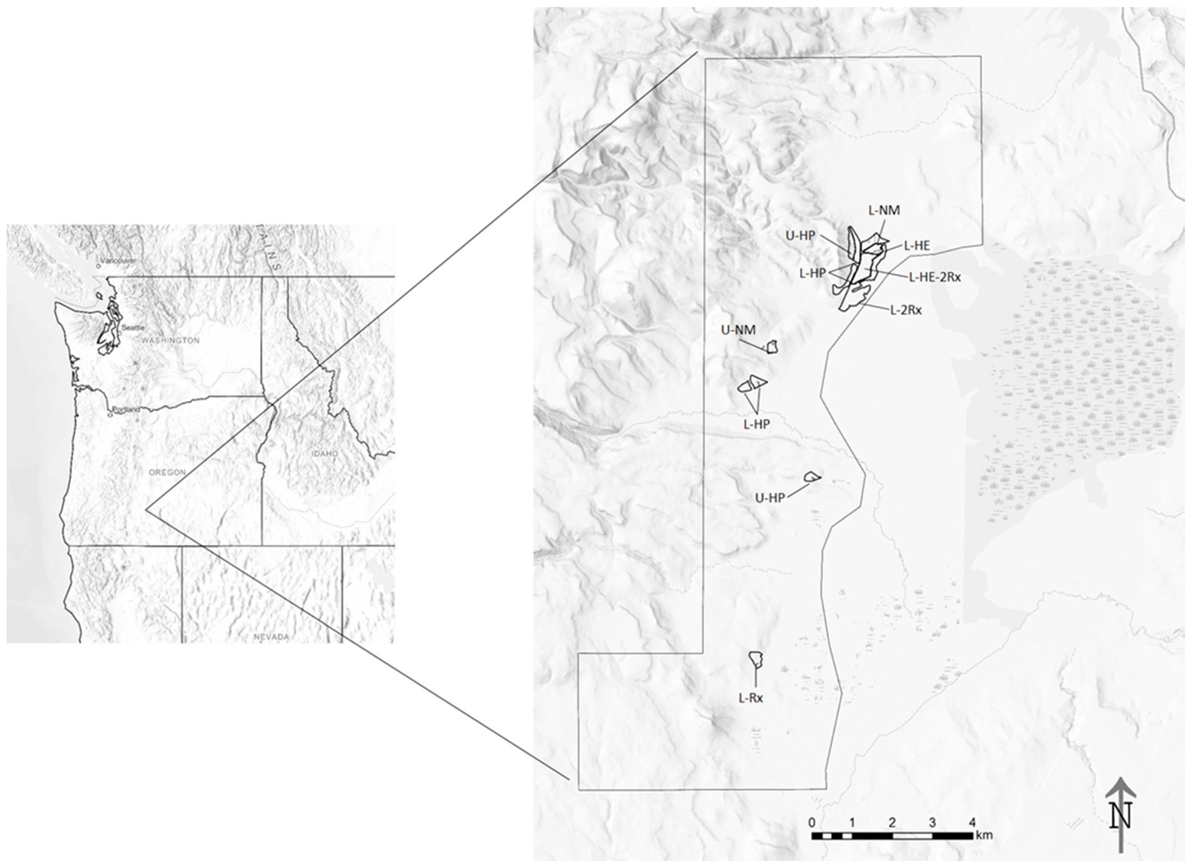
References

  1. Hann, W.; Jones, J.; Karl, M.; Hessburg, P.; Keane, R.; Long, D.; Menakis, J.; McNicoll, C.; Leonard, S.; Gravenmier, R.; et al. Landscape dynamics of the Basin. In An Assessment of Ecosystem Components in the Interior Columbia Basin and Portions of the Klamath and Great Basins: Volume II; Pacific Northwest Research Station, Forest Service, U.S. Department of Agriculture: Portland, OR, USA, 1997; pp. 338–1055. [Google Scholar]
  2. Simpson, M. Forested Plant Associations of the Oregon East Cascades; U.S. Department of Agriculture, Forest Service, Pacific Northwest Region: Portland, OR, USA, 2007. [Google Scholar]
  3. Oswalt, S.; Smith, B.U.S. Forest Resource Facts and Historical Trends. FS-1035 2014; U.S. Department of Agriculture, Forest Service: Portland, OR, USA, 2014; Volume 64. [Google Scholar]
  4. Hankin, L.E.; Higuera, P.E.; Davis, K.T.; Dobrowski, S.Z. Impacts of growing-season climate on tree growth and post-fire regeneration in ponderosa pine and Douglas-fir forests. Ecosphere 2019, 10, e02679. [Google Scholar] [CrossRef] [Green Version]
  5. Grulke, N.E. Plasticity in physiological traits in conifers: Implications for response to climate change in the western U.S. Environ. Pollut. 2010, 158, 2032–2042. [Google Scholar] [CrossRef]
  6. Agee, J.K. Fire Ecology of Pacific Northwest Forests; Island Press: Washington, DC, USA, 1993; ISBN 1-55963-230-5. [Google Scholar]
  7. Fitzgerald, S. Fire Ecology of Ponderosa Pine and the Rebuilding of Fire-Resilient Ponderosa Pine Ecoystems. In Proceedings of the PSW-GTR-198; USDA Forest Service: Klamath Falls, OR, USA, 2005; pp. 197–225. [Google Scholar]
  8. Zhang, J.; Finley, K.A.; Johnson, N.G.; Ritchie, M.W. Lowering Stand Density Enhances Resiliency of Ponderosa Pine Forests to Disturbances and Climate Change. For. Sci. 2019, 65, 496–507. [Google Scholar] [CrossRef]
  9. DeSoto, L.; Cailleret, M.; Sterck, F.; Jansen, S.; Kramer, K.; Robert, E.M.R.; Aakala, T.; Amoroso, M.M.; Bigler, C.; Camarero, J.J.; et al. Low growth resilience to drought is related to future mortality risk in trees. Nat. Commun. 2020, 11, 545. [Google Scholar] [CrossRef]
  10. Littell, J.S.; Peterson, D.L.; Riley, K.L.; Liu, Y.; Luce, C.H. A review of the relationships between drought and forest fire in the United States. Glob. Chang. Biol. 2016, 22, 2353–2369. [Google Scholar] [CrossRef] [PubMed]
  11. Sohn, J.A.; Saha, S.; Bauhus, J. Potential of forest thinning to mitigate drought stress: A meta-analysis. For. Ecol. Manag. 2016, 380, 261–273. [Google Scholar] [CrossRef]
  12. Keen, F.P. Keen’s Tree Classification and Marking Rules for Ponderosa Pine in B.C.; Technical Publication; Management Division, British Columbia Forest Service: Vancouver, BC, USA, 1951. [Google Scholar]
  13. Keen, F.P.; Salman, K.A. Progress in Pine Beetle Control through Tree Selection. J. For. 1942, 40, 854–858. [Google Scholar] [CrossRef]
  14. Bannari, A.; Morin, D.; Bonn, F.; Huete, A.R. A review of vegetation indices. Remote Sens. Rev. 1995, 13, 95–120. [Google Scholar] [CrossRef]
  15. Huete, A.; Liu, H.; Batchily, K.; van Leeuwen, W. A comparison of vegetation indices over a global set of TM images for EOS-MODIS. Remote Sens. Environ. 1997, 59, 440–451. [Google Scholar] [CrossRef]
  16. Tucker, C.J. Red and photographic infrared linear combinations for monitoring vegetation. Remote Sens. Environ. 1979, 8, 127–150. [Google Scholar] [CrossRef] [Green Version]
  17. Jiang, Z.; Huete, A.; Didan, K.; Miura, T. Development of a two-band enhanced vegetation index without a blue band. Remote Sens. Environ. 2008, 112, 3833–3845. [Google Scholar] [CrossRef]
  18. Huete, A.R. A soil-adjusted vegetation index (SAVI). Remote Sens. Environ. 1988, 25, 295–309. [Google Scholar] [CrossRef]
  19. Xue, J.; Su, B. Significant Remote Sensing Vegetation Indices: A Review of Developments and Applications. J. Sens. 2017, 2017, 1–17. [Google Scholar] [CrossRef] [Green Version]
  20. Filippa, G.; Cremonese, E.; Migliavacca, M.; Galvagno, M.; Sonnentag, O.; Humphreys, E.; Hufkens, K.; Ryu, Y.; Verfaillie, J.; di Cella, U.M.; et al. NDVI derived from near-infrared-enabled digital cameras: Applicability across different plant functional types. Agric. For. Meteorol. 2018, 249, 275–285. [Google Scholar] [CrossRef]
  21. Reid, A.M.; Chapman, W.K.; Prescott, C.E.; Nijland, W. Using excess greenness and green chromatic coordinate colour indices from aerial images to assess lodgepole pine vigour, mortality and disease occurrence. For. Ecol. Manag. 2016, 374, 146–153. [Google Scholar] [CrossRef]
  22. Martin, L.; Howarth, P. Change-detection accuracy assessment using SPOT multispectral imagery of the rural-urban fringe. Remote Sens. Environ. 1989, 30, 55–66. [Google Scholar] [CrossRef]
  23. Zhang, L.; Sun, X.; Wu, T.; Zhang, H. An Analysis of Shadow Effects on Spectral Vegetation Indexes Using a Ground-Based Imaging Spectrometer. IEEE Geosci. Remote Sens. Lett. 2015, 12, 2188–2192. [Google Scholar] [CrossRef]
  24. Navulur, K. Multispectral Image Analysis Using the Object-Oriented Paradigm; CRC Press: Boca Raton, FL, USA, 2006; ISBN 978-0-429-14630-5. [Google Scholar]
  25. Feret, J.-B.; Asner, G.P. Tree Species Discrimination in Tropical Forests Using Airborne Imaging Spectroscopy. IEEE Trans. Geosci. Remote Sens. 2013, 51, 73–84. [Google Scholar] [CrossRef]
  26. Wagner, F.H.; Ferreira, M.P.; Sanchez, A.; Hirye, M.C.M.; Zortea, M.; Gloor, E.; Phillips, O.L.; de Souza Filho, C.R.; Shimabukuro, Y.E.; Aragão, L.E.O.C. Individual tree crown delineation in a highly diverse tropical forest using very high resolution satellite images. ISPRS J. Photogramm. Remote Sens. 2018, 145, 362–377. [Google Scholar] [CrossRef]
  27. Lee, J.; Cai, X.; Lellmann, J.; Dalponte, M.; Malhi, Y.; Butt, N.; Morecroft, M.; Schonlieb, C.-B.; Coomes, D.A. Individual Tree Species Classification From Airborne Multisensor Imagery Using Robust PCA. IEEE J. Sel. Top. Appl. Earth Obs. Remote Sens. 2016, 9, 2554–2567. [Google Scholar] [CrossRef] [Green Version]
  28. Maschler, J.; Atzberger, C.; Immitzer, M. Individual Tree Crown Segmentation and Classification of 13 Tree Species Using Airborne Hyperspectral Data. Remote Sens. 2018, 10, 1218. [Google Scholar] [CrossRef] [Green Version]
  29. Ke, Y.; Quackenbush, L.J. A review of methods for automatic individual tree-crown detection and delineation from passive remote sensing. Int. J. Remote Sens. 2011, 32, 4725–4747. [Google Scholar] [CrossRef]
  30. Silván-Cárdenas, J.L. A Segmentation Method for Tree Crown Detection and Modelling from LiDAR Measurements. In Pat-tern Recognition; Carrasco-Ochoa, J.A., Martínez-Trinidad, J.F., Olvera López, J.A., Boyer, K.L., Eds.; Springer: Berlin/Heidelberg, Germany, 2012; Volume 7329, pp. 65–74. ISBN 978-3-642-31148-2. [Google Scholar]
  31. Vega, C.; Hamrouni, A.; Mokhtari, S.; Morel, J.; Bock, J.; Renaud, J.-P.; Bouvier, M.; Durrieu, S. PTrees: A point-based approach to forest tree extraction from lidar data. Int. J. Appl. Earth Obs. Geoinf. 2014, 33, 98–108. [Google Scholar] [CrossRef]
  32. Grulke, N.; Bienz, C.; Hrinkevich, K.; Maxfield, J.; Uyeda, K. Quantitative and qualitative approaches to assess tree vigor and stand health in dry pine forests. For. Ecol. Manag. 2020, 465, 118085. [Google Scholar] [CrossRef]
  33. Bienz, C.; Parsons, R.; Grulke, N.; Sauerbrey, K.; Rosendaul, K. Sharing the Road: Managers and Scientists Transforming Fire Management; Hood, S.M., Drury, S., Steelman, T., Steffens, R., Eds.; U.S. Department of Agriculture, Forest Service, Rocky Mountain Research Station: Fort Collins, CO, USA; Missoula, MT, USA, 2019; Volume RMRS-P-78, pp. 9–21. [Google Scholar]
  34. U.S. Drought Monitor Map Archive. Available online: https://droughtmonitor.unl.edu/Maps/MapArchive.aspx (accessed on 26 October 2020).
  35. USDA Forest Service Fremont-Winema National Forest Plant Association—ScienceBase-Catalog. Available online: https://www.sciencebase.gov/catalog/item/51d44f79e4b09630fbdc5301 (accessed on 5 October 2020).
  36. Churchill, D.J.; Larson, A.J.; Dahlgreen, M.C.; Franklin, J.F.; Hessburg, P.F.; Lutz, J.A. Restoring forest resilience: From reference spatial patterns to silvicultural prescriptions and monitoring. For. Ecol. Manag. 2013, 291, 442–457. [Google Scholar] [CrossRef]
  37. North, M.; Stine, P.; O’Hara, K.; Zielinski, W.; Stephens, S. An Ecosystem Management Strategy for Sierran Mixed-Conifer Forests; U.S. Department of Agriculture, Forest Service, Pacific Southwest Research Station: Albany, CA, USA, 2009; p. PSW-GTR-220. [Google Scholar]
  38. Shaw, R.C. Tree Vigor Response and Competitive Zone Density in Mature Ponderosa Pine; Oregon State University: Corvallis, OR, USA, 2017. [Google Scholar]
  39. Grulke, N.E. The physiological basis of ozone injury assessment attributes in Sierran conifers. In Developments in Environmental Science; Ozone Air Pollution in the Siera Nevada: Distribution and Effects on Forests; Elsevier: Amsterdam, The Netherlands, 2003; Volume 2, pp. 55–81. [Google Scholar]
  40. Grulke, N.E.; Lee, E.H. Assessing Visible Ozone-Induced Foliar Injury in Ponderosa Pine. Can. J. For. Res. 1997, 27, 1658–1668. [Google Scholar] [CrossRef]
  41. Staszak, J.; Grulke, N.E.; Marrett, M.J.; Prus-Glowacki, W. Isozyme markers associated with O3 tolerance indicate shift in genetic structure of ponderosa and Jeffrey pine in Sequoia National Park, California. Environ. Pollut. 2007, 149, 366–375. [Google Scholar] [CrossRef]
  42. Grulke, N.; Maxfield, J.; Riggan, P.; Schrader-Patton, C. Pre-Emptive Detection of Mature Pine Drought Stress Using Multispectral Aerial Imagery. Remote Sens. 2020, 12, 2338. [Google Scholar] [CrossRef]
  43. R Core Team. R: A Language and Environment for Statistical Computing; R Core Team: Vienna, Austria, 2017. [Google Scholar]
  44. Sandau, R. Examples of Large-Scale Digital Airborne Cameras. In Digital Airborne Camera; Springer: Dutch, The Netherlands, 2010; pp. 279–331. ISBN 978-1-4020-8877-3. [Google Scholar]
  45. Gillespie, A.R.; Kahle, A.B.; Walker, R.E. Color enhancement of highly correlated images. II. Channel ratio and “chromaticity” transformation techniques. Remote Sens. Environ. 1987, 22, 343–365. [Google Scholar] [CrossRef]
  46. Sonnentag, O.; Hufkens, K.; Teshera-Sterne, C.; Young, A.M.; Friedl, M.; Braswell, B.H.; Milliman, T.; O’Keefe, J.; Richardson, A.D. Digital repeat photography for phenological research in forest ecosystems. Agric. For. Meteorol. 2012, 152, 159–177. [Google Scholar] [CrossRef]
  47. Esri Inc. ArcGIS Pro (Version 2.5); Environmental Systems Research Institute (ESRI): Redlands, CA, USA, 2018. [Google Scholar]
  48. Hoaglin, D.C.; John, W. Tukey and Data Analysis. Stat. Sci. 2003, 18, 311–318. [Google Scholar] [CrossRef]
  49. Cutler, D.R.; Edwards, T.C.; Beard, K.H.; Cutler, A.; Hess, K.T.; Gibson, J.; Lawler, J.J. Random forests for classification in ecology. Ecology 2007, 88, 2783–2792. [Google Scholar] [CrossRef] [PubMed]
  50. Matsuki, K.; Kuperman, V.; Van Dyke, J.A. The Random Forests statistical technique: An examination of its value for the study of reading. Sci. Stud. Read. 2016, 20, 20–33. [Google Scholar] [CrossRef] [PubMed] [Green Version]
  51. Busse, M.D.; Cochran, P.H.; Hopkins, W.E.; Johnson, W.H.; Riegel, G.M.; Fiddler, G.O.; Ratcliff, A.W.; Shestak, C.J. Developing resilient ponderosa pine forests with mechanical thinning and prescribed fire in central Oregon’s pumice region. Can. J. For. Res. 2009, 39, 1171–1185. [Google Scholar] [CrossRef] [Green Version]
  52. Latham, P.; Tappeiner, J. Response of old-growth conifers to reduction in stand density in western Oregon forests. Tree Physiol. 2002, 22, 137–146. [Google Scholar] [CrossRef] [Green Version]
  53. McDowell, N.; Brooks, J.R.; Fitzgerald, S.A.; Bond, B.J. Carbon isotope discrimination and growth response of old Pinus ponderosa trees to stand density reductions: Effects of Reduced Stand Density on Pinus Ponderosa Trees. Plant Cell Environ. 2003, 26, 631–644. [Google Scholar] [CrossRef]
  54. Restaino, C.; Young, D.J.N.; Estes, B.; Gross, S.; Wuenschel, A.; Meyer, M.; Safford, H. Forest structure and climate mediate drought-induced tree mortality in forests of the Sierra Nevada, USA. Ecol. Appl. 2019, 29, e01902. [Google Scholar] [CrossRef] [PubMed]
  55. Zhang, J.; Ritchie, M.W.; Maguire, D.A.; Oliver, W.W. Thinning ponderosa pine (Pinus ponderosa) stands reduces mortality while maintaining stand productivity. Can. J. For. Res. 2013, 43, 311–320. [Google Scholar] [CrossRef] [Green Version]
  56. Hatten, J.; Zabowski, D.; Ogden, A.; Theis, W.; Choi, B. Role of season and interval of prescribed burning on ponderosa pine growth in relation to soil inorganic N and P and moisture. For. Ecol. Manag. 2012, 269, 106–115. [Google Scholar] [CrossRef]
  57. Skov, K.R.; Kolb, T.E.; Wallin, K.F. Tree Size and Drought Affect Ponderosa Pine Physiological Response to Thinning and Burning Treatments. For. Sci. 2004, 50, 81–91. [Google Scholar] [CrossRef]
  58. McNulty, S.G.; Boggs, J.L.; Sun, G. The rise of the mediocre forest: Why chronically stressed trees may better survive extreme episodic climate variability. New For. 2014, 45, 403–415. [Google Scholar] [CrossRef]
  59. He, Y.; Weng, Q. High Spatial Resolution Remote Sensing: Data, Analysis, and Applications; CRC Press: Boca Raton, FL, USA, 2018; ISBN 978-0-429-89299-8. [Google Scholar]
  60. Karlson, M.; Reese, H.; Ostwald, M. Tree Crown Mapping in Managed Woodlands (Parklands) of Semi-Arid West Africa Using WorldView-2 Imagery and Geographic Object Based Image Analysis. Sensors 2014, 14, 22643–22669. [Google Scholar] [CrossRef] [PubMed]
  61. Baldeck, C.A.; Asner, G.P.; Martin, R.E.; Anderson, C.B.; Knapp, D.E.; Kellner, J.R.; Wright, S.J. Operational Tree Species Mapping in a Diverse Tropical Forest with Airborne Imaging Spectroscopy. PLoS ONE 2015, 10, e0118403. [Google Scholar] [CrossRef]
  62. Dalponte, M.; Frizzera, L.; Gianelle, D. Individual tree crown delineation and tree species classification with hyperspectral and LiDAR data. PeerJ 2019, 6, e6227. [Google Scholar] [CrossRef] [PubMed]
  63. Marconi, S.; Graves, S.J.; Gong, D.; Nia, M.S.; Le Bras, M.; Dorr, B.J.; Fontana, P.; Gearhart, J.; Greenberg, C.; Harris, D.J.; et al. A data science challenge for converting airborne remote sensing data into ecological information. PeerJ 2019, 6, e5843. [Google Scholar] [CrossRef] [Green Version]
  64. Persson, M.; Lindberg, E.; Reese, H. Tree Species Classification with Multi-Temporal Sentinel-2 Data. Remote Sens. 2018, 10, 1794. [Google Scholar] [CrossRef] [Green Version]
  65. Chen, Q.; Baldocchi, D.; Gong, P.; Kelly, M. Isolating Individual Trees in a Savanna Woodland Using Small Footprint Lidar Data. Photogramm. Eng. Remote Sens. 2006, 72, 923–932. [Google Scholar] [CrossRef] [Green Version]
  66. Eitel, J.U.H.; Vierling, L.A.; Litvak, M.E.; Long, D.S.; Schulthess, U.; Ager, A.A.; Krofcheck, D.J.; Stoscheck, L. Broadband, red-edge information from satellites improves early stress detection in a New Mexico conifer woodland. Remote Sens. Environ. 2011, 115, 3640–3646. [Google Scholar] [CrossRef]
Figure 1. Map of our study area (8824 ha) in south–central Oregon. Elevations ranged from 1520 m to 1719 m. Locations of stands in the study area where trees were sampled are presented in the large-scale map on the right. Key to stand codes: L = lowland, U = upland, HE = harvest, even spacing, HP = harvest, patchy (clumps and openings), Rx = prescribed fire, NM = no management, no harvest or fire.
Forests 12 00612 g001
Figure 2. Examples of qualitative visual characteristics used to assess trees to vigor classes. (A) The tree on the right exhibits chlorosis and low needle retention, while the tree on the left has good needle color and mass, (B) reduced needle elongation and fading, (C) needle senescence, and (D) low needle retention (from [32]).
Forests 12 00612 g002
Figure 3. Aerial imagery collected in October 2017 (four (R, G, B, IR) bands, 30 cm resolution) with classified individual tree crowns (red = low vigor, blue = not low vigor). This image contains four different site treatments; on the upper right is L-NM, lower right L-HE-2Rx, left of the main road is L-HP, and between the two spur roads on the right is L-HE.
Forests 12 00612 g003
Figure 4. Graph of variable importance produced by the Random Forest model. Vertical axis values are the predictor variables and the horizontal axis shows the decrease in model accuracy if the variable is removed.
Forests 12 00612 g004
Figure 5. Graph of the proportion of LOW tree crowns (ITCs) in the eight stands with standard error. Stands that are not significantly different (two tailed Z-score tests of a proportion, p > 0.01) have the same italicized letter (ae). For example, U-NM and L-Rx, are not significantly different; U-HP, L-2Rx and L-HE are not significantly different. Stand treatment descriptions are as follows: U-NM is upland, no management; L-Rx is lowland prescribed fire (2008); L-HP is lowland, harvest in 2016, retention of trees in groups; L-NM is lowland, no management; U-HP is upland, harvest in 2016, retention of trees in groups; L-2Rx is lowland, prescribed fire in 2006 and 2013; L-HE is lowland, harvest even spacing; and L-HE-2Rx is lowland, harvest even spacing, prescribed fire in 2006 and 2013.
Forests 12 00612 g005
Table 1. Description of stands in the study area where trees were sampled. Key to stand codes: L = lowland, U = upland, HE = harvest, even spacing, HP = harvest, patchy (clumps and openings), Rx = prescribed fire, NM = no management, no harvest or fire. Diameter at breast height (1.37 m above ground, DBH), BA (basal area), and trees per hectare (TPH) data from [32]. These data are based on the DBH and species of each tree in three 30 m radius plots in each site. Values are the mean ± SD. PP = ponderosa pine. N/A indicates that no belt transects were conducted in these stands.
StandHarvestRx BurnMean DBH (cm)PP BA (m2/ha)All Species BA (m2/ha)PP TPHAll Species TPH
U-NMN/AN/A35.2 ± 4.061.4 ± 80.461.4 ± 80.4559 ± 361559 ± 361
U-HP2016N/A34.6 ± 3.534.8 ± 15.034.8 ± 15.0307 ± 50307 ± 50
L-NMN/AN/A21.2 ± 1.727.6 ± 12.830.0 ± 13.8605 ± 237722 ± 289
L-HP2016N/A41.2 ± 2.818.6 ± 4.918.6 ± 4.9160 ± 36160 ± 36
L-HE2005N/A37.5 ± 0.88.8 ± 3.88.8 ± 3.8137 ± 57137 ± 57
L-HE-2Rx20052006,
2013
38.5 ± 1.817.3 ± 5.717.3 ± 5.7146 ± 16146 ± 16
L-RxN/A200823.9 ± 1.65.51 ± 1.016.0 ± 1.2434 ± 22566 ± 14
L-2RxN/A2006, 201341.4 ± 1.928 ± 8.028 ± 8.0160 ± 36160 ± 36
Table 2. Whole-tree and branch characteristics used in assigning qualitative-vigor classes to ponderosa pine individual tree crowns (ITCs). DMR is the dwarf mistletoe rating.
LOWNOT LOW
Low number of whorls—low needle retention.Highest number of whorls—high needle retention.
High level of needle chlorosis, fading, yellowing.Low or no visible needle chlorosis, no visible fading.
Thinner branchlets.Thicker branchlets.
High frequency of early needle senescence (browning).Low frequency of early needle senescence (browning).
Low needle mass.High needle mass.
High DMR rank.Low DMR rank.
Table 3. Spectral indices calculated from the four-band imagery and used in the vigor model and classification of Ponderosa pine individual tree crowns (ITCs). NIR = near-infrared band, R = red band, B = blue band, G = green band.
IndexFormulaCitation
Normalized Differential Vegetation Index (NDVI)(NIR-R)/(NIR ± R)Rouse et al., 1974; Tucker 1979
Enhanced Vegetation Index (EVI)2.5(NIR-R)/(NIR ±(2.4R) ±1)Jiang et al., 2008.
Difference Vegetation Index (DVI)NIR-RRichardson and Wiegand 1977.
Blue Chromatic Coordinate (BCC)B/(R ± G ± B)Gillespie et al., 1987; Stafford 2015.
Red Chromatic Coordinate (RCC)R/(R ± G ± B)Gillespie et al. 1987; Stafford 2015.
Green Chromatic Coordinate (GCC)G/(R ± G ± B)Gillespie et al., 1987; Stafford 2015; Reid et al., 2016.
Table 4. Individual tree crown (ITC) spectra/index attribute values (MEAN and SE) for trees in the two vigor classes. Marked (*) attributes are significantly different (p < 0.05) between the LOW and NOT LOW vigor classes using the Mann–Whitney test for differences in means. Indices defined: DVI = difference vegetation index; NDVI = normalized differential vegetation index; EVI=enhanced vegetation index; RCC = red chromatic coordinate; BCC = blue chromatic coordinate; GCC = green chromatic coordinate. SD indicates the standard deviation of the pixels within an ITC. For example, GREEN SD is the standard deviation of the green value of all the pixels within an ITC.
SPECTRA/INDEXLOWNOT LOWp-Value
BLUE_MEAN124 (0.27)124 (0.24)0.85
RED_MEAN143 (0.45)143 (0.35)0.68
GREEN_MEAN145 (0.37)146 (0.29)0.42
NIR MEAN *221 (0.31)222 (0.24)0.0057
DVI MEAN *77 (0.40)78 (0.33)0.0089
NDVI MEAN *0.21 (0.0013)0.21 (0.0010)0.039
EVI MEAN *0.34 (0.0023)0.34 (0.0019)0.036
RCC MEAN *0.35 (0.00036)0.35 (0.00026)0.012
BCC MEAN0.30 (0.00033)0.30 (0.00022)0.997
GCC MEAN0.35 (0.00024)0.35 (0.00017)0.0011
BLUE SD *2.7 (0.12)3.4 (0.076)0.0000088
RED SD *4.2 (0.16)5.1 (0.11)0.000024
GREEN SD *3.9 (0.15)4.5 (0.092)0.0097
NIR SD5.0 (0.23)5.4 (0.15)0.14
NIRR SD *4.1 (0.23)5.0 (0.14)0.00036
NDVI SD *0.012 (0.00060)0.015 (0.00038)0.000018
EVI SD *0.021 (0.0010)0.026 (0.00066)0.000014
RCC SD *0.0026 (0.00010)0.0032 (7.8 × 10⁻⁵)0.0000076
BCC SD *0.0027 (9.9 × 10⁻⁵)0.0029 (6.1 × 10⁻⁵)0.026
GCC SD *0.0020 (6.8 × 10⁻⁵)0.0023 (4.9 × 10⁻⁵)0.0053
Table 5. Tree-vigor attribute values (MEANS and SE) for trees in the two vigor classes. Marked (*) attributes significantly differed (p < 0.05) using the Wilcoxon rank sum test. Tree-vigor attribute attributes were defined as follows: WHL is the number of years needles retained; BRDIA2 is the previous year branchlet diameter (±/− 0.01mm); BRLN1 is the current year branchlet length (±/− 2.0 mm); %MxNL1 is the current-year needle length relative to the longest needles produced on the branchlet; CHL4 is the level of chlorosis in 4-year-old needles; LF BI DF is a synthetic index of foliar (biotic) insect defoliators (including summed frequency of weevil, unknown phloem feeders, and scale); LF A DF is the summed frequency of needle tip dieback, dead needles, and early senescence; DMR is the dwarf mistletoe rating [32].
RANKWHL *BRDIA2BRLN1%MxNL1CHL4 *LF BI DFLF A DFDMR
NOT LOW6.3 (0.09)6.1 (0.10)14 (0.54)89.9 (0.89)8 (1.0)2.7 (0.05)0.67 (0.05)0.0 (0.10)
LOW6.0 (0.2)5.7 (0.21)13 (1.1)89 (1.7)13 (3.8)2.3 (0.14)1 (0.12)0.0 (0.27)
Table 6. OOB (out of bag) error matrix for the Random Forest model vigor predictions for all ITCs (individual tree crowns, outliers removed). The columns are the crowns as predicted by the model and the rows are the vigor assessments made in the field (reference data). The overall accuracy of 0.78 is calculated as the number of correctly classified crowns divided by the total number of crowns. The KAPPA statistic is the overall accuracy adjusted for random correct classification.
LOWNOT LOWROW TOTALUSERS ACCURACYError of Commission (Type II)
LOW33691020.320.68
NOT LOW182512690.930.07
COLUMN TOTAL51320371
PRODUCERS ACCURACY0.650.78
Error of Omission (Type I)0.350.22
ACCURACY:0.77
KAPPA STATISTIC:0.30
Table 7. Proportion of LOW RF-modeled individual tree crowns (ITCs) in upland and lowland sites. The proportion of LOW crowns was significantly different (two tailed Z-score tests of a proportion, p = 0.023) for the two site types.
LOWNOT LOWTOTALLOW/All Crowns
Lowland509619855249510.20
Upland1768641981870.22
Table 8. Proportion of LOW trees in each stand type as determined by the Random Forest model using spectral data (RF model), field qualitative assessment of the belt transect trees (n = 108) and 298 additional trees (All trees), and field qualitative assessment of 30 trees in a belt transect (Belt transect trees). Stand codes are L = lowland; U = upland; HP = harvested, patchy; HE = harvested, even spacing; NM = no management, Rx = prescribed burn. N/A indicates that no belt transects were conducted in this stand.
STANDRF ModelAll TreesBelt Transect Trees
U-NM0.320.200.18
U-HP0.180.240.18
L-NM0.260.350.40
L-HP0.220.610.05
L-HE0.160.280.13
L-HE-2Rx0.140.040.07
L-Rx0.340.35N/A
L-2Rx0.20.140.07
Publisher’s Note: MDPI stays neutral with regard to jurisdictional claims in published maps and institutional affiliations.

