Temporal Dynamics of Root Reinforcement in European Spruce Forests

Abstract

The quantification of post-disturbance root reinforcement (RR) recovery dynamics is of paramount importance for the optimisation of forest ecosystem services and natural hazards risk management in mountain regions. In this work we analyse the long-term root reinforcement dynamic of spruce forests combining data of the Swiss National Forest Inventory with data on root distribution and root mechanical properties. The results show that root reinforcement recovery depends primarily on stand altitude and slope inclination. The maximum root reinforcement recovery rate is reached at circa 100 years. RR increases continuously with different rates for stand ages over 200 years. These results shows that RR in spruce stands varies considerably depending on the local conditions and that its recovery after disturbances requires decades. The new method applied in this study allowed for the first time to quantify the long term dynamics of RR in spruce stands supporting new quantitative approaches for the analysis of shallow landslides disposition in different disturbance regimes of forests.

1. Introduction

In mountain regions, many forests protect human settlements and activities against gravitational natural hazards [1]. At the same time, forest ecosystems worldwide are increasingly perturbed by climate-driven natural disturbances [2], which may determine a temporary reduction in the provision of forest ecosystem services, including protection from natural hazards [3]. One of the priorities of forest management is therefore to avoid or shorten temporary gaps in forest’s protective effectiveness following forest fires or stand-replacing silvicultural interventions (e.g., coppicing, clearcutting) [4,5]. Given the limited resources for forest management, prioritizing silvicultural measures based on the long-term dynamics of forest ecosystems and their protective effect may be of paramount importance in the context of an integrated risk management of natural hazards [1].

The relationship between post-disturbance root reinforcement recovery dynamics in a forest stand and the hazards of shallow landslides is a prime and documented example in this context. The long-term dynamics of root reinforcement in mountain forest management has important implications for the decision makers, not only for post-disturbance management measures but also for optimising forest ecosystem services of forests in general. Post-event time windows of increased shallow landslide disposition may range from a few years [3,6] to several decades [5,7] depending on the disturbance severity, tree species concerned, and site characteristics. While the recovery of vegetation cover in the short term has in general an important effect in reducing the runoff in the contribution area of a potential landslide and in the related effect on building of pore water pressure [8], in the long term, root reinforcement becomes the dominant factor for slope stability in areas of potential shallow landslides [9,10].

A large number of studies quantify the short-term dynamics of root reinforcement after a disturbance in forest stands [3,11,12,13,14] considering both changes in the spatiotemporal distribution of roots [13,15] and the change in their mechanical properties due to decay [16,17]. Vergani et al. [18] showed that after a stand-replacing fire in scots pine (Pinus Sylvestris) stands, the reduction in root reinforcement efficiency was mainly due to the loss of the mechanical properties (such as tensile strength and stiffness) of coarse roots, implying the total loss of the reinforcement within 5–10 years. Similar rates of decay have been reported following clearcut coppicing [19]. Studies dealing with dynamics of root reinforcement recovery are very rare [4]. Ziemer [20] reported that a 50% recovery of root reinforcement was reached within 15–25 years after clearcutting of lodgepole pine (Pinus contorta). Gehring et al. [14] found that the gap in protection against shallow landslides due to the loss of root reinforcement in beech (Fagus sylvatica) stands following wildfires may extend over 35 years in case of medium to high severity fires. Liu et al. [10] showed that the recovery of root reinforcement in the first four post-disturbance years in closed forest stands at high altitudes (i.e., 1800 m a.s.l.) was slow or almost absent, suggesting that spruce stands at this altitude need particular attention for the study of root reinforcement dynamics in the long term.

In this paper, we analyse the long-term dynamics of root reinforcement in spruce forests (Picea abies). This species is known to have a relatively low specific root reinforcement compared to other tree species such as beech or chestnut (Castanea sativa) [14,19,21]. However, spruce is the most common tree species of the reported Alpine protective forest area [22], being dominant in Swiss and Austrian protective forests [23,24]. Moreover, spruce is considered one of the most sensitive species to the ongoing climate change and is expected to be increasingly vulnerable to disturbances in future decades [25], particularly due to drought stress and bark beetle outbreaks [26,27]. In addition, in its upper natural mountain range, spruce forests usually display slow stand dynamics and regeneration rates [28,29]. In the context of an integrated forest management in the Alpine region, analytical models for the quantification of post-disturbance root reinforcement dynamic of this species are particularly needed in assessing future protective capacity, as well as for planning silvicultural measures.

The aim of this paper is thus to characterise the long-term root reinforcement dynamics of spruce forests along an altitude gradient by assessing the post-disturbance recovery of lateral root reinforcement at the stand scale. To this purpose, we combined data of the Swiss National Forest Inventory (Swiss NFI) and other European forest inventories with published data on root distribution and root mechanical properties of spruce to calibrate the Root Bundle Model [30] and to upscale the related root reinforcement effect at stand scale [14,21].

2. Materials and Methods

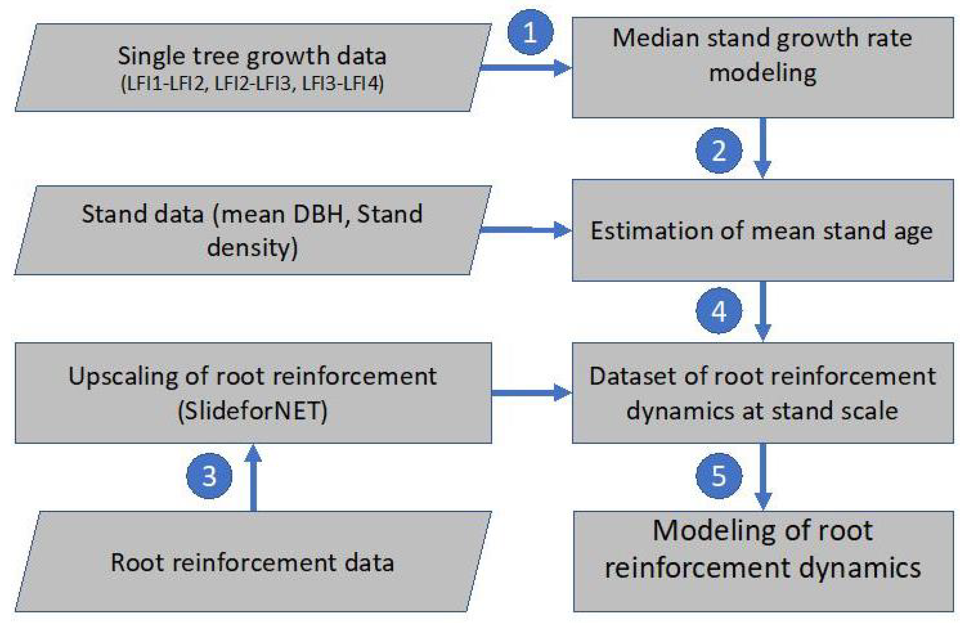
2.1. Workflow and Methodological Approaches

The flowchart in Figure 1 shows the overall methodological steps needed for the calculation of the long-term root reinforcement dynamics at the stand scale. In the first step, we test different single tree growth models to predict the mean annual diameter at breast height (DBH) increment of spruce trees using as reference Swiss NFI trees. In a second step, we calibrate a stand-scale model for the estimation of mean stand age based on observed forest structure and mean tree size (stem diameter). In the third step, stand characteristics and root reinforcement data are combined to calculate the lateral root reinforcement at stand scale. The calculated root reinforcement at the stand scale is then paired to the corresponding stand ages. Finally, in a fifth step, the temporal dynamics of root reinforcement are calculated using an empirical model.

2.2. Data Sources

Long-term spruce stands data are retrieved from the Swiss NFI and other European forest inventories. For about 40 years, the Swiss NFI has collected data at tree as well as at stand level using systematic and well-described methods [31,32]. The first Swiss NFI (NFI1) was conducted between 1983 and 1985, followed by three additional surveys in 1993–1995 (NFI2), 2004–2006 (NFI3), and 2009–2017 (NFI4). Since 2009, data have been collected over a nine-year period. Currently, the fifth inventory is underway from 2018 to 2026 (NFI5). The terrestrial data of NFI1 were collected on some 11,000 plots located on a systematic 1 km × 1 km grid covering the entire country [33]. Since NFI2 the number of sample plots is reduced, and field measurements are conducted on a 1.4 km × 1.4 km subgrid of the NFI1 grid resulting on about 6500 forest plots in NFI4. On each plot, two concentric circles (i.e., 200 m${}^2$ and 500 m${}^2$ in size, respectively) are defined to measure all trees and shrubs with a DBH between 12 cm and 36 cm in the inner circle, respectively, and all trees with a DBH larger than 36 cm in the outer one [33].

Site characteristics such as altitude, aspect, and slope as well as the stand density index (SDI) were also retrieved from Swiss NFI data to be used as explanatory variables for modeling the DBH growth of individual trees. SDI is defined by Reineke et al. [34] using the allometric coefficient described in Schütz and Zingg [35]. Tree density (number of stems per hectare) and mean size (quadratic mean DBH) were also collected from the Swiss NFI for the upscaling of the root reinforcement at stand level. Furthermore, 2640 plots from Italy, Germany, Czech Republic, and France were included in order to compare the results of the Swiss stands with values obtained for the rest of the continent [36]. This dataset is named “European” in this manuscript.

Data on spruce root distribution and mechanical properties (maximum tensile strength and apparent secant stiffness) were retrieved from published studies on root reinforcement of spruce stands [13,37,38]. The spatial distribution of roots in spruce stands was calculated following Schwarz et al. [21] using data from 95 soil profiles in six different locations in Switzerland [37,38]. The mechanical properties of roots were quantified based on 93 field pull-out tests described in Vergani et al. [37] and Moos et al. [38].

2.3. Stem Diameter Growth Modelling

To quantify the average DBH growth of spruce trees under the existing Swiss environmental conditions, we built a simplified model using diameter increment data of more than 50,600 individuals belonging to 8631 spruce-dominated plots and measured in at least two consecutive Swiss NFI inventories (i.e., NFI1-NFI2, NFI2-NFI3, NFI3-NFI4). We defined spruce-dominated stands as Swiss NFI-plots with at least 80% of the basal area represented by spruce trees.

In our modeling approach, we first modelled tree growth as a function of individual tree DBH and then refined the model using stand and site parameters such as SDI, altitude, aspect, and slope, implementing either a nonlinear [29] or a linear modeling approach.

The mean annual tree diameter increment (in cm) at the stand scale can be considered as the approximation of a continuous growth rate, i.e.,

$$MeanAnnualDiameterGrowth = \frac{\Delta DBH}{\Delta \tau }\sim \frac{dDHB}{d\tau }$$

(1)

where $\tau$ represents the beginning time of the measurements of the DBH. If we denote by t the age (years) of a spruce tree, we have that:

$$t = \tau + c_{1.3}$$

(2)

where $c_{1.3}$ is the mean time needed by seedlings to reach 1.3 m height.

Data for the estimation of $c_{1.3}$ were sourced from an unpublished dataset from the Swiss Alps [39], containing totally 231 spruce. The spruce at <1200 m.a.s.l. reaches 1.3 m height in 9 years, while this time increases to 12 and 17 years respectively for high montane (1200–1600 m.a.s.l.) and subalpine forests (1600–2100 m).

We present hereafter two suitable models to model DBH growth. The nonlinear model (NLM) is based on the Gompertz function:

$${\displaystyle \frac{dDBH}{d\tau }} = {\beta }_{1}DBH + {\beta }_{2}DBH·lnDBH + {\epsilon }_{error}$$

(3)

where ${\beta }_1$ and ${\beta }_2$ are model coefficients. We consider a small error term ${\epsilon }_{error}\approx 0$ and take as initial measurement:

$$DBH(\tau = 0) = {\epsilon }_{DBH} > 0$$

(4)

i.e., the measured initial DBH of the spruce at the age $t = \tau + c_{1.3}$ years is small but different from 0. NLM will not allow to use a more simplified initial condition and then reduce all to ${\epsilon }_{DBH} = 0$. Imposing ${\epsilon }_{DBH} = 0$ the differential equation will lead to the trivial solution $DBH\left(\tau \right) = 0$ for all $\tau > 0$.

Equation (3) is equivalent to:

$${\displaystyle \frac{dDBH}{d\tau }} = -r·DBH·ln{\displaystyle \frac{DBH}{K}}$$

(5)

where r indicates the growth rate and K the carrying capacity (or upper asymptote for growth). Relations among coefficients of Equations (3) and (5) are as follows:

$${\beta }_1 = r·lnKand{\beta }_2 = -r$$

(6)

$$K = e^{-{\displaystyle \frac{{\beta }_1}{{\beta }_2}}}andr = -{\beta }_2.$$

(7)

According to Schelhaas et al. [29] the parameters ${\beta }_1$ and ${\beta }_2$ are dependent upon a number of environmental and site variables:

$${\displaystyle {\beta }_1 = c_1 + \sum _{i=1}^p{\theta }_{i,1}·X_i = c_1 + {\theta }_{1,1}slope + {\theta }_{2,1}altitude + {\theta }_{3,1}aspect + {\theta }_{4,1}SDI}$$

(8)

$${\displaystyle {\beta }_2 = c_2 + \sum _{i=1}^p{\theta }_{i,2}·X_i}$$

(9)

where ${\theta }_{i,2}$ is a weighted array of model coefficients. This approach allows the weighting of individual variables ($X_i$) to be discussed in a multivariable model.

The analytical solution of this model is given by:

$$DBH\left(\tau \right) = K·e^{c·e^{-r·\tau }}$$

(10)

where C is the constant related to the initial condition $DBH\left(0\right) = {\epsilon }_{BHD}$:

$$C = ln{\displaystyle \frac{DBH\left(0\right)}{K}} = ln{\displaystyle \frac{{\epsilon }_{DBH}}{K}}$$

(11)

The linear model (LM) proposed as a simplification of NLM:

$${\displaystyle \frac{dDBH}{d\tau }} = {\beta }_1 + {\beta }_2·DBH$$

(12)

Since the measurement of DBH begins at $\tau = 0$ (i.e., at age $c_{1.3}$ years, when the spruce reaches the height of 1.3 m) we have again:

$$DBH(\tau = 0) = {\epsilon }_{DBH} > 0.$$

(13)

One of the advantages of LM is the possibility to use a suitable simplified approximated initial condition without losing the sense of the growth process: we can here impose $DBH(\tau = 0) = 0$. This initial condition makes sense even if inserted in Equation (12):

$${\displaystyle \frac{dDBH}{d\tau }}(\tau = 0) = {\beta }_1 + {\beta }_2·DBH(\tau = 0) = {\beta }_1$$

(14)

The “initial” growth rate at $\tau = 0$ of the spruce tree is given by the strictly positive coefficient ${\beta }_1$.

The general solution of the classical ordinary linear differential Equation (12) is:

$$DBH\left(\tau \right) = C·e^{{\beta }_2·\tau } - {\displaystyle \frac{{\beta }_1}{{\beta }_2}}$$

(15)

where

$$C = DBH(\tau = 0) + {\displaystyle \frac{{\beta }_1}{{\beta }_2}} = 0 + {\displaystyle \frac{{\beta }_1}{{\beta }_2}} = {\displaystyle \frac{{\beta }_1}{{\beta }_2}}$$

(16)

From (15) and (16), we obtain

$$DBH\left(\tau \right) = {\displaystyle \frac{{\beta }_1}{{\beta }_2}}·(e^{{\beta }_2·\tau } - 1)$$

(17)

where parameters ${\beta }_1$ and ${\beta }_2$ were again determined using Formulas (8) and (9) for NLM.

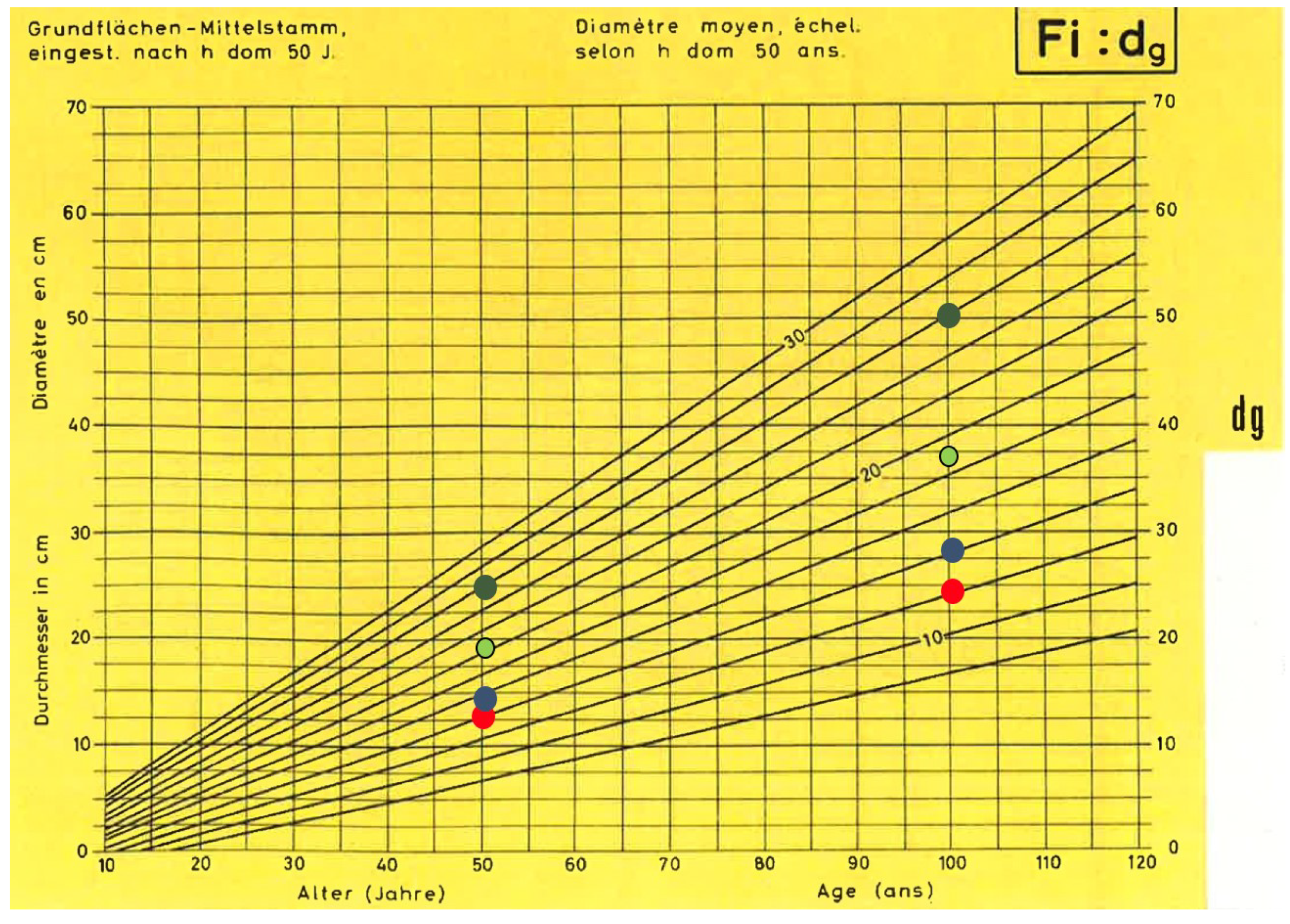
2.4. Estimation of Mean Stand Age

Considering Equation (14) and its solution (17) to the mean annual DBH growth rate of the stand, it is possible to determine a formula for $\tau$. In particular, it is possible to represent the mean age of a spruce stand as a function of its quadratic mean diameter (QMD):

$$\tau = {\displaystyle \frac{1}{{\beta }_2}}·ln\left({\displaystyle \frac{{\beta }_2}{{\beta }_1}}·QMD + 1\right)$$

(18)

The age of the stand, t (years), is therefore:

$$age = t = \tau + c_{1.3} = {\displaystyle \frac{1}{{\beta }_2}}·ln\left({\displaystyle \frac{{\beta }_2}{{\beta }_1}}·QMD + 1\right) + c_{1.3}$$

(19)

2.5. Upscaling of Root Reinforcement

The Root Bundle Model-Weibull (RBMw) was used as a basis for the calculation of the root reinforcement at tree and upscaled to stand level following Schwarz et al. [21], as described in Vergani et al. [13] and most recently in Gehring et al. [14]. The upscaling consists of two parts. On one hand, (1), roots of several trees are counted and measured for their thickness in soil trenches at different distance from tree stems. On the other hand, (2), the mechanical properties, tensile strength, and apparent secant stiffness of the roots are needed to determine the maximum pulling force of the roots [30,40]. The root mechanical properties for different root diameter (up to 40 mm) are determined by field pull-out tests [13,19,38,41].

From these parameters (i.e., number of roots and root mechanical properties) a model of the maximum tensile force at the level of a single tree root system can be generated.

The maximum root reinforcement $RRmax$ is calculated with the following formula implemented in the SlideforNET model [14,15]:

$$RRmax(DBH,d) = a·DBH·\mathsf{\Gamma }\left(\frac{d}{DBH·18.5},b,c\right)\mathrm{for}d < DBH·18.5$$

(20)

$$RRmax(DBH,d) = 0\mathrm{for}d > DBH·18.5$$

(21)

where $\mathsf{\Gamma }$ stands for the gamma distribution, and d [m] for the distance from the stem base. The coefficients a, b and c are species-specific. For spruce these are: $a =$ 276,601.4, $b = 0.0122$, $c = 0.00468$. The correlation coefficient of the fit is 0.6 and the residual standard error is 6530 N/m.

For upscaling to stand level, the number of trees per hectare and the quadratic mean tree diameter are used. It is assumed that the trees are homogeneous and distributed over the area in a triangular grid. The value of $RRmax$ calculated for the largest distance between two trees is used as root reinforcement of the stand. This should represent the weakest point of the root network at the stand scale. Thus, the model uses the pessimistic value (minimum) of root reinforcement at stand scale.

To quantify root reinforcement, stand data from the Swiss NFI surveys were used. The lateral root reinforcement was calculated from the 7191 (filtered from the original 8631, considering only stand with $RRmax > 0$) stands using the corresponding input parameters and SlideforNET.

2.6. Model for the Temporal Dynamics of Root Reinforcement after Disturbances

The data on calculated stand age (Section 2.3 and Section 2.4) and the data on upscaled stand root reinforcement (Section 2.5) were used to model the recovery of root reinforcement as function of time since disturbance. The model is based on the cumulative distribution function of the two parameter Weibull distribution:

$$RR = (s\_1 + q1·slope + q2·altitude)\left(1 - exp\left(-{\left({\displaystyle \frac{age}{\lambda }}\right)}^k\right)\right)$$

(22)

where $s\_1$, $q1$, $q2$, k, and $\lambda$ are coefficients fitted after Schelhaas et al. [29].

The coefficients of the model were fitted using the nls() function of the R software [42]. The upper and lower 95% prediction interval were calculated using standardized residuals [43], in order to consider heteroscedasticity. Age 0 is considered as the year of first establishment of spruce regeneration after a disturbance, which may depend on the type of successional dynamics that takes place at any specific site.

3. Results

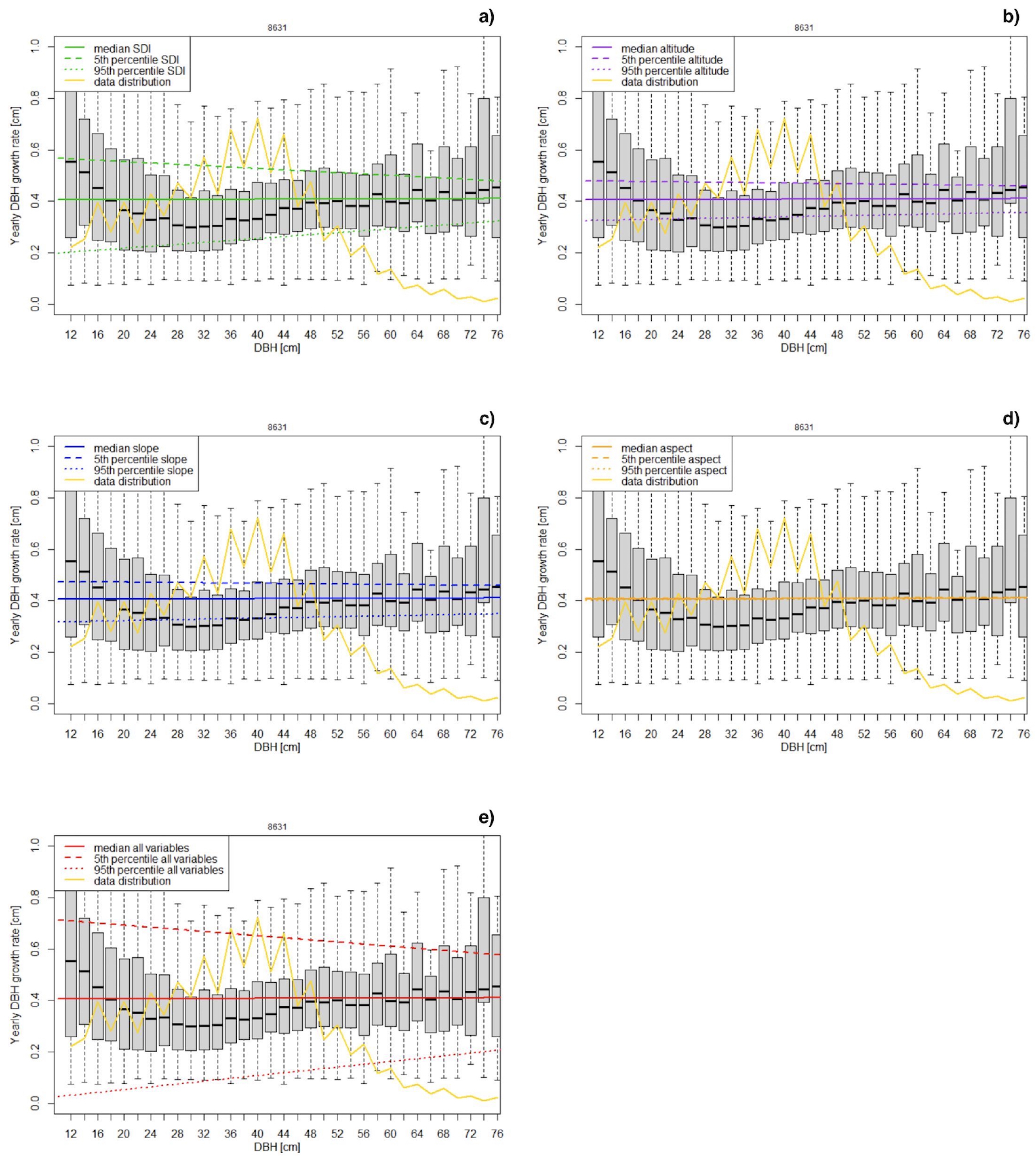
3.1. Modeling of Growth Rate

Based on the analysis of the Swiss NFI data, the yearly diameter growth of single spruce trees ranges between 0.1 and 1 cm/year. The overall median value is 0.305 cm/year, whereas the mean value is 0.377 cm/year. Most of the data refer to a range of DBH of single trees between 25 and 50 cm. The results of the model fitting show that the performance of the two models (NLM and LM) are similar as well as the significance of the model variables (

Table 1. Coefficients of the NLM. RMSE = 0.2207 cm/year on 8621 degrees of freedom.

Coefficient	Value	Std Error	Error t-Value	p-Value
Slope x1	$-2.819 \times {10}^{-4}$	$2.928 \times {10}^{-5}$	−9.631	<0.001
Altitude x2	$-1.674 \times {10}^{-5}$	$2.025 \times {10}^{-6}$	−8.267	<0.001
Aspect x3	$1.062 \times {10}^{-5}$	$1.413 \times {10}^{-5}$	0.751	0.452
SDI x4	$-4.993 \times {10}^{-5}$	$2.329 \times {10}^{-6}$	−21.438	<0.001
Slope y1	$6.637 \times {10}^{-5}$	$7.763 \times {10}^{-6}$	8.550	<0.001
Altitude y2	$3.865 \times {10}^{-6}$	$4.579 \times {10}^{-7}$	9.502	<0.001
Aspect y3	$4.974 \times {10}^{-7}$	$3.156 \times {10}^{-6}$	−0.771	0.441
SDI y4	$1.031 \times {10}^{-5}$	$5.279 \times {10}^{-7}$	19.523	<0.001
c_1	$1.120 \times {10}^{-1}$	$2.822 \times {10}^{-3}$	39.694	<0.001
c_2	$-2.528 \times {10}^{-2}$	$7.494 \times {10}^{-4}$	−33.740	<0.001

and

Table 2. Coefficient of the LM. RMSE = 0.2207 cm/year on 8621 degrees of freedom.

Coefficient	Value	Std Error	Error t-Value	p-Value
Slope x1	$-2.033 \times {10}^{-3}$	$2.695 \times {10}^{-4}$	−7.543	<$2 \times {10}^{-16}$
Altitude x2	$-1.301 \times {10}^{-4}$	$1.783 \times {10}^{-5}$	−7.299	<$2 \times {10}^{-16}$
Aspect x3	$-5.059 \times {10}^{-5}$	$1.246 \times {10}^{-4}$	−0.406	0.6848
SDI x4	$-4.255 \times {10}^{-4}$	$2.086 \times {10}^{-5}$	−20.400	<0.001
Slope y1	$1.671 \times {10}^{-5}$	$7.129 \times {10}^{-6}$	2.343	0.0191
Altitude y2	$1.164 \times {10}^{-6}$	$4.754 \times {10}^{-7}$	2.449	0.0144
Aspect y3	$8.503 \times {10}^{-7}$	$3.223 \times {10}^{-6}$	0.264	0.7919
SDI y4	$6.143 \times {10}^{-6}$	$5.461 \times {10}^{-7}$	11.249	<0.001
c$\_1$	$9.049 \times {10}^{-1}$	$2.388 \times {10}^{-2}$	37.885	<0.001
c$\_2$	$5.751 \times {10}^{-3}$	$6.393 \times {10}^{-4}$	−8.996	<0.001

). For both models the SDI is the most important parameter, followed by slope and altitude. Aspect has no statistically significant influence on growth rate.

Overall, assuming a median value for each predictor, LM predicts an almost constant growth rate of about 0.4 cm/year (Figure 2). The variability of model results decreases with increasing DBH.

In view of these results, we chose to drop the “aspect” predictor (see

Table 3. Coefficient of the LM without aspect. RMSE = 0.2109 cm/year with 8623 degrees of freedom.

Coefficient	Value	Std Error	Error t-Value	p-Value
Slope x1	$-2.035 \times {10}^{-3}$	$2.694 \times {10}^{-4}$	−7.553	$4.70 \times {10}^{-14}$
Altitude x2	$-1.306 \times {10}^{-4}$	$1.780 \times {10}^{-5}$	−7.339	$2.34 \times {10}^{-13}$
SDI x4	$-4.257 \times {10}^{-4}$	$2.084 \times {10}^{-5}$	−20.429	<0.001
Slope y1	$1.678 \times {10}^{-5}$	$7.127 \times {10}^{-6}$	2.355	0.0186
Altitude y2	$1.170 \times {10}^{-6}$	$4.747 \times {10}^{-7}$	2.466	0.0137
SDI y4	$6.147 \times {10}^{-6}$	$5.453 \times {10}^{-7}$	11.272	<0.001
c_1	$9.014 \times {10}^{-1}$	$2.231 \times {10}^{-2}$	40.411	<0.001
c_2	$-5.691 \times {10}^{-3}$	$6.019 \times {10}^{-4}$	−9.455	<0.001

for coefficient) and to use LM for further analyses.

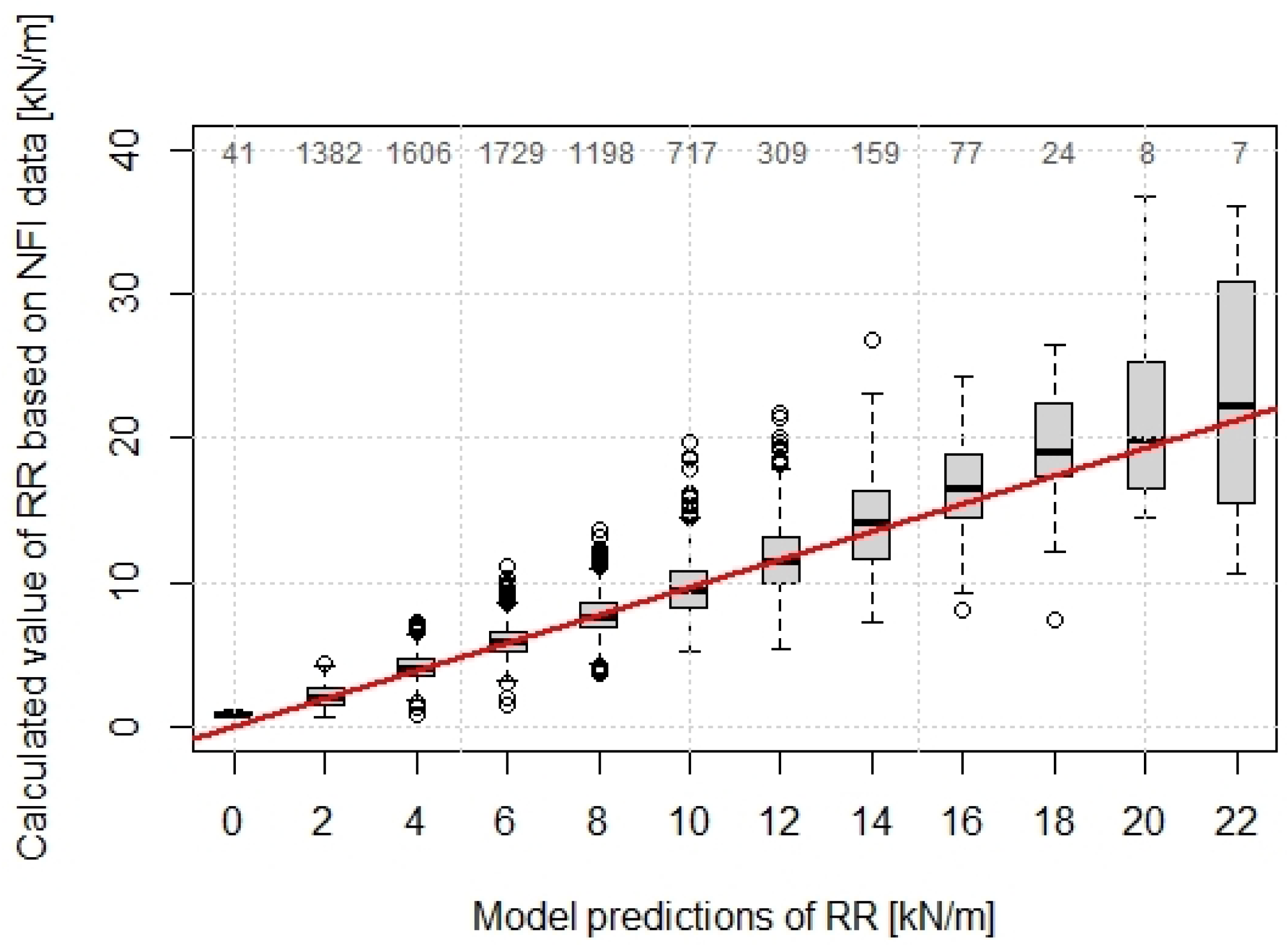
3.2. Calculation of Root Reinforcement

The information on mean DBH and stem density for each stand were used to calculate the minimum values of lateral root reinforcement at the stand scale for the Swiss NFI and European datasets (Figure 3). The two ranges of root reinforcement overlap up to a DBH class of about 50 cm, while for larger DBH the returned root reinforcement was higher in the European dataset. In general, lateral root reinforcement of spruce stands in Europe can be expected to be linearly proportional to the mean DBH of the stand and to have values up to ca. 30 kN/m.

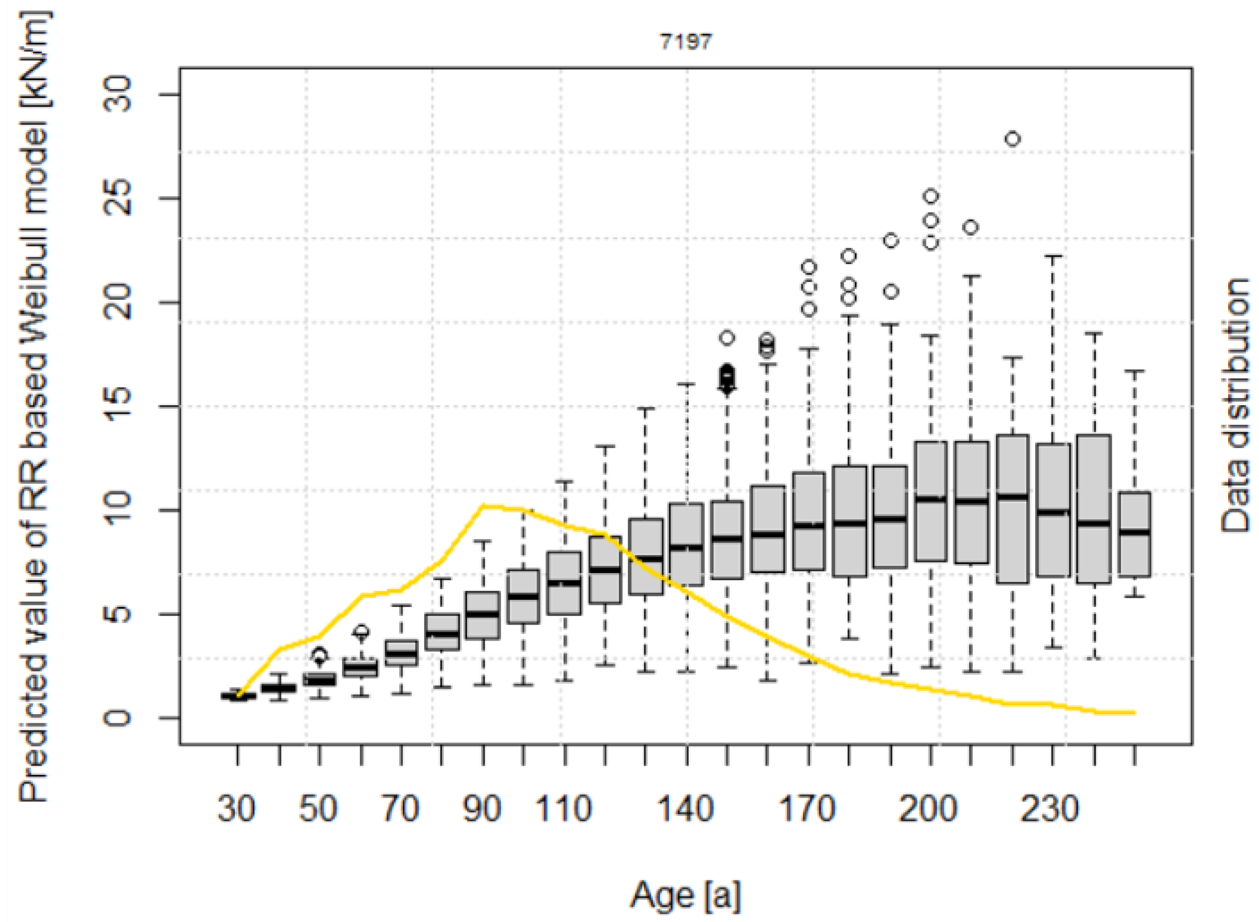
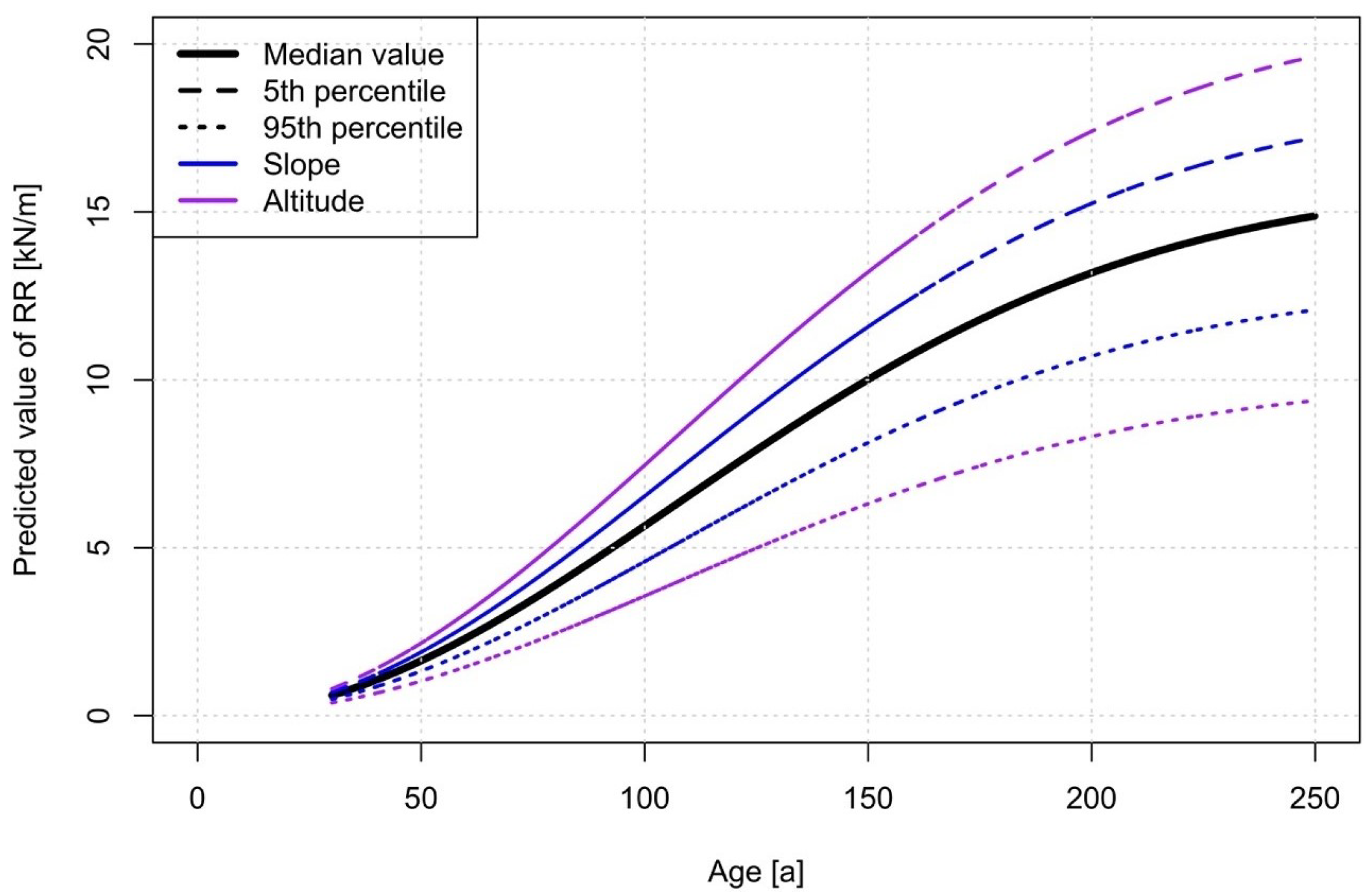
3.3. Modelling Root Reinforcement Dynamic

The calculated lateral root reinforcement (Equation (19)) increases continuously with increasing stand age up to median values of about 10 kN/m at 200 years (Figure 4). 50% of the root reinforcement values (i.e., from the 25% to the 75% quantiles) for stand ages higher than 150 years range between 6 and 13 kN/m.

All the parameters of the RR~age model have a p-value lower than 0.001 (

Table 4. Coefficient of the RR~age model. The RMSE has a value of 1.738 kN/m on 7192 degrees of freedom.

Coefficient	Value	Std Error	Error t-Value	p-Value
$q1$	−0.06986	0.0027	−25.98	<0.001
$q2$	−0.0085	0.0002	−39.38	<0.001
lambda	150.04	2.7191	55.18	<0.001
k	2.017	0.0293	68.79	<0.001
s_1	27.87	0.5932	46.99	<0.001

), indicating a statistically significant influence on the results. The negative values of the coefficient $q1$ and $q2$ indicate that lateral root reinforcement decreases with increasing altitude and slope. The scaling factor $\lambda$ of the Weibull distribution has a value of 150, and the shape parameter k is 2.017.

The variability of the predicted values increases with increasing root reinforcement, whereby up to values of 12 kN/m, the range of 50% predicted values is in the range of approximately 2 kN/m (Figure 5).

A sensitivity analysis in accord to Schelhaas et al. [29] of the RR~age model shows that altitude influenced the results up to approximately 30% of their median value, whereas the slope influences up to approximately 15% (Figure 6). The inflection point of the curve is at 106 years (corresponding to the mode value of the Weibull cumulative distribution).

4. Discussion

4.1. Comparison of the Two Growth Rate Models

The two models applied to describe the DBH increment in this paper are related to the classical topic in the mathematics of differential equation for population growth models. The choice of a model to fit a growth process can be done stepwise considering which type of complexity can be afforded and at the same time, which prediction accuracy is requested for the model applications. The use of a linear model is considered in general to give a good approximation of an initial growing phase or for a very slow growth process. Vice versa, “logistic“ or “Gompertz” models are expected to fit better for more complex growing behaviours [29,44]. The very large dataset considered in the analysis supports, within the aim of this study, the linear growth model approximation to perform best, allowing us to reduce the model complexity by however achieving a suited prediction accuracy. In our specific case, incertitudes due to the 1 cm measurements accuracy of the DBH are compensated by the high number of trees measured and the years between two inventories. The linear behaviour of the growth rate data in this work is influenced by two additional characteristics: firstly, measurements are taken for trees with DBH > 12 cm, meaning that the usually higher growth rate of the first years is not considered, and secondly, the growth rate is calculated as the mean considering the DBH increment of single trees over 4–6 years, leading to a smoothing of the annual growth rate, especially in the first years.

In selecting the model variables we paid attention to inserting only easily measurable parameters in order to make the proposed approach useful for practical applications such as the assessment of forest recovery after disturbances. As a result, we ended up with a reduced number of variables in comparison to Schelhaas et al. [29] and we used for instance the easy retrievable altitude instead of the correlated temperature data. However, our approach makes it more difficult to project current dynamics into the climate change scenarios. Nevertheless, present studies did not reveal significant changes in the growth rate of spruce along altitude gradients in the European Alps, indicating no climate change effects so far [45].

In the model, the SDI for the estimation of the stand age is considered as a static variable, although it may change over time in reality. In the scope of this work, however, the SDI calculated from the Swiss NFI data is considered representative for predicting the root reinforcement dynamics after a disturbance. Future studies on this topic could implement more variables such as soil properties and type of forest management to improve the performance of the growth rate model. The competition between trees and climate extremes considerably influences the growth rate and eventually also the survival chance of single individuals [46]. However, the effects of self-thinning mechanisms and/or silvicultural interventions have in general small and limited-in-time impacts on the overall growth rate of spruce stands [47,48]. Considering the results by Uhl [49], this behaviour seems limited to less productive sites, whereas in favourable conditions for spruce, single trees show significant growth increment after thinning.

Based on the NFI data used for calibration, the proposed model assumes site specific optimisation of the overall stand growth rate at the stand scale, which results from the balancing competition for resources and the related population densities [34]. Pretzsch et al. [50] discussed the reaction pattern of forest stands or cohorts as more than just the growth response of individual trees depending on their competition for resources. The results of our study for spruce show a complete symmetry of growth rate versus single tree size (DBH). This result could be interpreted as a stronger competition of trees for limited below-ground resources (independently of the tree size) [51] and less than competition for light (which is expected to lead to a stronger correlation between growth rate and single tree dimension). Pretzsch et al. [50] state that “simulations for archetypical stands yield a transition from size-asymmetric to size-symmetric competition along the gradient from fertile to poor sites”. In combination with our results, this statement leads to the conclusion that spruce in the NFI dataset tend to compete for soil resources, more than for light. A detailed analysis of dendrochronological data could be used in future works to further investigate these aspects.

4.2. Correlation between Mean DBH and Stand Age

The general trend of a constant growth rate is confirmed by the linear correlation between age and mean DBH of dominant trees in a stand, as reported in yield tables for spruce [52]. Figure 7 compares model results of this work with the different growing classes (“Bonitäten”, growing potential of the tree species on a given site) of the Swiss yield tables. Similar trends are shown in Stöcker [53], Ammann [54], Schelhaas et al. [55], Simmler [56], and Kindermann et al. [57]. Castagneri et al. [58] obtained DBH~age curves of single spruce trees in Norway from dendrochronological analysis. Their results show that fast growing young trees generally tend to die, whereas older trees have a more regular linear growth. This supports the conclusion that mean growing rate of forest stand is dominated in the long term by trees with a constant linear growth. The results of this study show that site altitude and slope can explain most of the growing capacity of the concerned spruce stands.

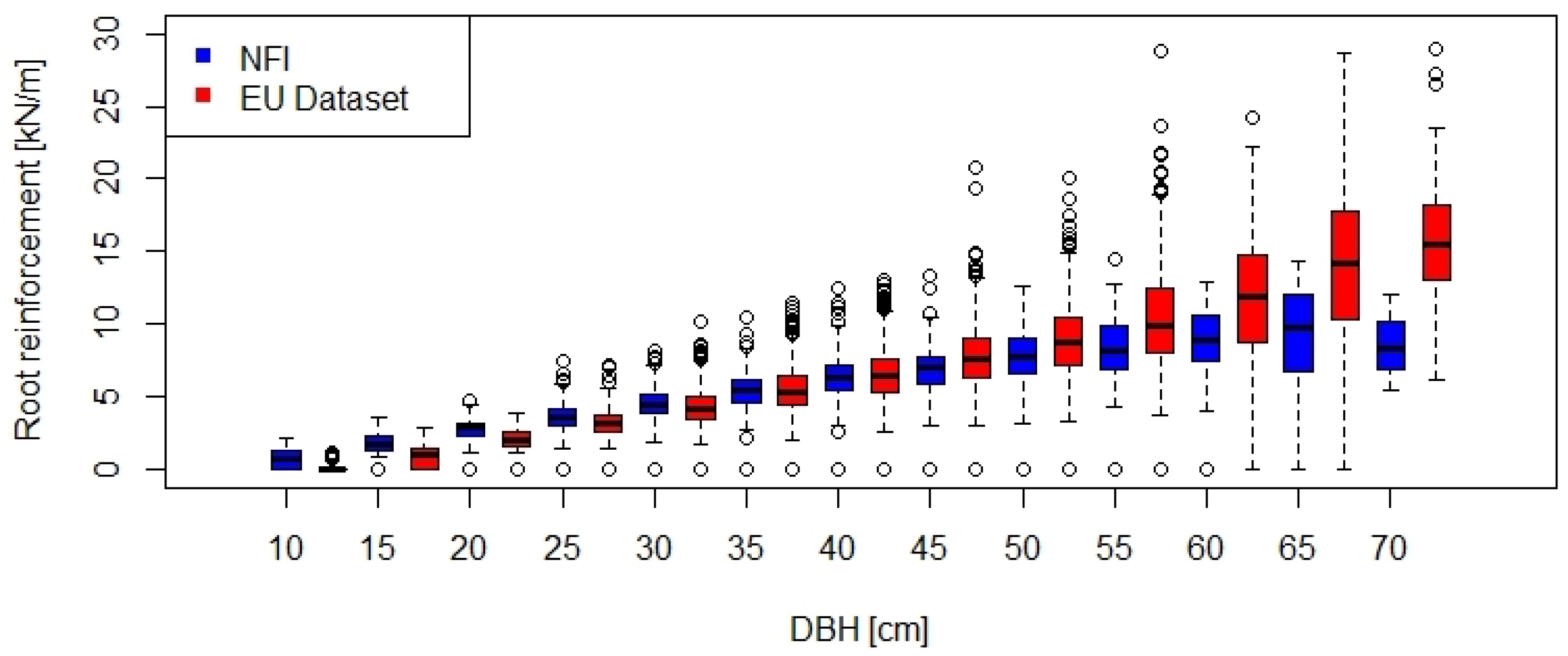
4.3. Upscaling of Root Reinforcement

We use the minimum lateral root reinforcement as a proxy variable for the characterisation of the mechanical effect of root on slope stability at the stand scale. In reality, lateral root reinforcement is highly variable within a stand, but potential tension cracks of a landslide can be assumed to follow the weakest paths within a stand. To improve and extend this calculation to the stabilization effect of roots, basal root reinforcement should be considered too. In contrast to the lateral reinforcement which acts on the vertical edge of a potential landslide, the basal root reinforcement interacts along the shear plane of a potential landslide (parallel to slope) [15]. The basal root reinforcement is thus strongly influenced by characteristics of the site [59,60] and the depth of the potential shear plane of a landslide [14,61]. In particular, in the case of very shallow landslides (with depth < 0.5 m) low values of lateral root reinforcement may result in high values of basal root reinforcement. High values of lateral root reinforcement may on the contrary result in a null basal root reinforcement if the landslide is deep enough. Gehring et al. [14] present an approach that shows the effect of different basal root reinforcement on slope stability.

In consideration of the variables used to calculate the lateral root reinforcement (mean stem DBH and mean distance between stems), it is important to mention that the dimension of the Swiss NFI plots can be considered big enough to be representative of a forest stand and small enough to avoid extreme heterogeneous pattern of vegetation cover and structures usually present in larger areas of forest.

4.4. Root Reinforcement Dynamics

The post-disturbance window of susceptibility for shallow landslides mainly depends on root decay of the dying trees, recovery rate of the new stand in terms of roots and canopy, and the frequency and magnitude of triggering rainfall events. Considering that total root decay is usually achieved in a temporal range of 5 to 15 years, the window of susceptibility can in general be expected to persist over 50 to 100 years. In reality, this temporal window tends to be shorter in stable areas (where landslides are triggered by extreme events only) and longer where high values of root reinforcement are needed to stabilise the slope. A detailed and spatial-explicit quantification of this effect is fundamental for an effective post-disturbance management that optimises investments of resources and mitigates the risks due to shallow landslides.

The evaluation of RR-recovery depends on the original conditions of a stand too. For example, Liu et al. [10] state that recovery in forest gaps is faster than in closed forest, whereby the term of comparison is completely different. For instance, in forest opening root reinforcement is dominated by small roots that regrow faster after disturbances due to grass regrowth and tree regeneration. Whereas, in old and close forest stands, decayed coarse roots need much more time to be replaced. Moreover, several publications confirm that the contribution of fine roots to the overall root reinforcement is negligible if coarse roots are present [10,41].

5. Conclusions

The results of this work show the possible range of root reinforcement dynamic calculated based on existing forest stands (Swiss NFI) in Switzerland. We do not know the “story” of each stand, but in general the upper boundary of the calculated root reinforcement can be considered as the maximum potential condition that an “ideal” forest can reach in function of time. In this case, the definition of the “ideal” forest considering the upper boundary of the estimated root reinforcement is considerably different from the one applied in the Swiss guidelines for protection forest management. While the latter is defined on the basis of ecological and structural characteristics of a forest stand (such as tree stability and the presence of renovation), in this work we propose a more quantitative approach based on the effect of the vegetation on the hazard process. This allows a better characterisation of the time required for a forest stand to recover its protection function and to evaluate the effectiveness of the protection function with respect to the potential of a stand. In reality, the recovery of the protective function of the forest is often influenced by many other factors (almost independently of the characteristics of the stand) such as the concurrence with other species (in some cases neophytes), the damages due to ungulates, the presence of seed trees, and the mobility of seeds.

References

1. Moos, C.; Bebi, P.; Schwarz, M.; Stoffel, M.; Sudmeier-Rieux, K.; Dorren, L. Ecosystem-based disaster risk reduction in mountains. Earth Sci. Rev. 2018, 177, 497–513. [Google Scholar] [CrossRef]
2. Seidl, R.; Thom, D.; Kautz, M.; Martin-Benito, D.; Peltoniemi, M.; Vacchiano, G.; Wild, J.; Ascoli, D.; Petr, M.; Honkaniemi, J.; et al. Forest disturbances under climate change. Nat. Clim. Chang. 2017, 7, 395–402. [Google Scholar] [CrossRef] [PubMed]
3. Vergani, C.; Giadrossich, F.; Buckley, P.; Conedera, M.; Pividori, M.; Salbitano, F.; Rauch, H.; Lovreglio, R.; Schwarz, M. Root reinforcement dynamics of European coppice woodlands and their effect on shallow landslides: A review. Earth Sci. Rev. 2017, 167, 88–102. [Google Scholar] [CrossRef]
4. Sidle, R.C. A conceptual model of changes in root cohesion in response to vegetation management. J. Environ. Qual. 1991, 20, 43–52. [Google Scholar] [CrossRef]
5. Saito, H.; Murakami, W.; Daimaru, H.; Oguchi, T. Effect of forest clear-cutting on landslide occurrences: Analysis of rainfall thresholds at Mt. Ichifusa, Japan. Geomorphology 2017, 276, 1–7. [Google Scholar] [CrossRef]
6. Rengers, F.K.; McGuire, L.A.; Oakley, N.S.; Kean, J.W.; Staley, D.M.; Tang, H. Landslides after wildfire: Initiation, magnitude, and mobility. Landslides 2020, 17, 2631–2641. [Google Scholar] [CrossRef]
7. Bebi, P.; Bast, A.; Ginzler, C.; Rickli, C.; Schöngrundner, K.; Graf, F. Waldentwicklung und flachgründige Rutschungen: Eine grossflächige GIS-Analyse. Schweiz. Z. Forstwes. 2019, 170, 318–325. [Google Scholar] [CrossRef]
8. Sidle, R.; Ochiai, H. Processes, prediction, and land use. In Water Resources Monograph; American Geophysical Union: Washington, DC, USA, 2006. [Google Scholar]
9. Kim, J.; Kim, Y.; Jeong, S.; Hong, M. Rainfall-induced landslides by deficit field matric suction in unsaturated soil slopes. Environ. Earth Sci. 2017, 76, 1–17. [Google Scholar] [CrossRef]
10. Liu, W.; Yang, Z.; He, S. Modeling the landslide-generated debris flow from formation to propagation and run-out by considering the effect of vegetation. Landslides 2021, 18, 43–58. [Google Scholar] [CrossRef]
11. O’loughlin, C.; Watson, A. Root-wood strength deterioration in radiata pine after clearfelling. NZJ For. Sci. 1979, 9, 284–293. [Google Scholar]
12. Preti, F. Forest protection and protection forest: Tree root degradation over hydrological shallow landslides triggering. Ecol. Eng. 2013, 61, 633–645. [Google Scholar] [CrossRef]
13. Vergani, C.; Schwarz, M.; Soldati, M.; Corda, A.; Giadrossich, F.; Chiaradia, E.A.; Morando, P.; Bassanelli, C. Root reinforcement dynamics in subalpine spruce forests following timber harvest: A case study in Canton Schwyz, Switzerland. Catena 2016, 143, 275–288. [Google Scholar] [CrossRef]
14. Gehring, E.; Conedera, M.; Maringer, J.; Giadrossich, F.; Guastini, E.; Schwarz, M. Shallow landslide disposition in burnt European beech (Fagus sylvatica L.) forests. Sci. Rep. 2019, 9, 1–11. [Google Scholar] [CrossRef]
15. Schwarz, M.; Preti, F.; Giadrossich, F.; Lehmann, P.; Or, D. Quantifying the role of vegetation in slope stability: A case study in Tuscany (Italy). Ecol. Eng. 2010, 36, 285–291. [Google Scholar] [CrossRef]
16. Ammann, M. Schutzwirkung Abgestorbener Bäume Gegen Naturgefahren; ETHZ: Zürich, Switzerland, 2006. [Google Scholar]
17. Zhu, J.; Wang, Y.; Wang, Y.; Mao, Z.; Langendoen, E.J. How does root biodegradation after plant felling change root reinforcement to soil? Plant Soil 2020, 446, 211–227. [Google Scholar] [CrossRef]
18. Vergani, C.; Werlen, M.; Conedera, M.; Cohen, D.; Schwarz, M. Investigation of root reinforcement decay after a forest fire in a Scots pine (Pinus sylvestris) protection forest. For. Ecol. Manag. 2017, 400, 339–352. [Google Scholar] [CrossRef]
19. Dazio, E.; Conedera, M.; Schwarz, M. Impact of different chestnut coppice managements on root reinforcement and shallow landslide susceptibility. For. Ecol. Manag. 2018, 417, 63–76. [Google Scholar] [CrossRef]
20. Ziemer, R. Roots and the stability of forested slopes. In Proceedings of the International Symposium on Erosion and Sediment Transport in Pacific Rim Steeplands, Christchurch, New Zealand, 25–31 January 1981; pp. 343–361. [Google Scholar]
21. Schwarz, M.; Cohen, D.; Or, D. Spatial characterization of root reinforcement at stand scale: Theory and case study. Geomorphology 2012, 171, 190–200. [Google Scholar] [CrossRef]
22. Lier, M.; Schuck, A.; Fischer, C.; Moffat, A.; Linser, S. Maintenance and appropriate enhancement of protective functions in forest management (notably soil and water). In State of Europe’s Forests 2020; UNECE: Geneva, Switzerland, 2020. [Google Scholar]
23. Brändli, U.; Abegg, M.; Allgaier Leuch, B. Schweizerisches Landesforstinventar: Ergebnisse der Vierten Erhebung 2009–2017. (Results of the Fourth Swiss National Forest Inventory 2009–2017); Swiss Federal Research Institute for Forest, Snow and Landscape Research, Birmensdorf (ZH) and Federal Office for the Environment (FOEN): Bern, Switzerland, 2020. [Google Scholar]
24. Büchsenmeister, R. Waldinventur 2007/09: Betriebe und Bundesforste nutzen mehr als den Zuwachs. BFW Praxisinf. 2011, 24, 6–9. [Google Scholar]
25. Hlásny, T.; Barka, I.; Roessiger, J.; Kulla, L.; Trombik, J.; Sarvašová, Z.; Bucha, T.; Kovalčík, M.; Čihák, T. Conversion of Norway spruce forests in the face of climate change: A case study in Central Europe. Eur. J. For. Res. 2017, 136, 1013–1028. [Google Scholar] [CrossRef]
26. Thiele, J.C.; Nuske, R.S.; Ahrends, B.; Panferov, O.; Albert, M.; Staupendahl, K.; Junghans, U.; Jansen, M.; Saborowski, J. Climate change impact assessment—A simulation experiment with Norway spruce for a forest district in Central Europe. Ecol. Model. 2017, 346, 30–47. [Google Scholar] [CrossRef]
27. Scherrer, D.; Ascoli, D.; Conedera, M.; Fischer, C.; Maringer, J.; Moser, B.; Nikolova, P.S.; Rigling, A.; Wohlgemuth, T. Canopy Disturbances Catalyse Tree Species Shifts in Swiss Forests. Ecosystems 2021. [Google Scholar] [CrossRef]
28. Mäkinen, H.; Nöjd, P.; Kahle, H.P.; Neumann, U.; Tveite, B.; Mielikäinen, K.; Röhle, H.; Spiecker, H. Radial growth variation of Norway spruce (Picea abies (L.) Karst.) across latitudinal and altitudinal gradients in central and northern Europe. For. Ecol. Manag. 2002, 171, 243–259. [Google Scholar] [CrossRef]
29. Schelhaas, M.J.; Hengeveld, G.M.; Heidema, N.; Thürig, E.; Rohner, B.; Vacchiano, G.; Vayreda, J.; Redmond, J.; Socha, J.; Fridman, J.; et al. Species-specific, pan-European diameter increment models based on data of 2.3 million trees. For. Ecosyst. 2018, 5, 1–19. [Google Scholar] [CrossRef]
30. Schwarz, M.; Giadrossich, F.; Cohen, D. Modeling root reinforcement using a root-failure Weibull survival function. Hydrol. Earth Syst. Sci. 2013, 17, 4367–4377. [Google Scholar] [CrossRef]
31. Brassel, P.; Brändli, U.B.; la Neige et le Paysage (Birmensdorf) Institut Fédéral de Recherches sur la Forêt; des Forêts et du Paysage Suisse Office Fédéral de l’Environnement. Swiss National Forest Inventory: Methods and Models of the Second Assessment; WSL: Birmensdorf, Switzerland, 2001. [Google Scholar]
32. Fischer, C.; Traub, B. Swiss National Forest Inventory-Methods and Models of the Fourth Assessment; Springer: Berlin/Heidelberg, Germany, 2019. [Google Scholar]
33. Lanz, A.; Abegg, M.; Braendli, U.B.; Camin, P.; Cioldi, F.; Ginzler, C.; Fischer, C. National Forest Inventories; Springer: Berlin/Heidelberg, Germany, 2016. [Google Scholar]
34. Reineke, L.H. Perfection a stand-density index for even-aged forest. J. Agric. Res. 1933, 46, 627–638. [Google Scholar]
35. Schütz, J.P.; Zingg, A. Improving estimations of maximal stand density by combining Reineke’s size-density rule and the yield level, using the example of spruce (Picea abies (L.) Karst.) and European Beech (Fagus sylvatica L.). Ann. For. Sci. 2010, 67, 507. [Google Scholar] [CrossRef]
36. Vacchiano, G.; Derose, R.J.; Shaw, J.D.; Svoboda, M.; Motta, R. A density management diagram for Norway spruce in the temperate European montane region. Eur. J. For. Res. 2013, 132, 535–549. [Google Scholar] [CrossRef]
37. Vergani, C.; Chiaradia, E.; Bassanelli, C.; Bischetti, G. Root strength and density decay after felling in a Silver Fir-Norway Spruce stand in the Italian Alps. Plant Soil 2014, 377, 63–81. [Google Scholar] [CrossRef]
38. Moos, C.; Bebi, P.; Graf, F.; Mattli, J.; Rickli, C.; Schwarz, M. How does forest structure affect root reinforcement and susceptibility to shallow landslides? Earth Surf. Process. Landf. 2016, 41, 951–960. [Google Scholar] [CrossRef]
39. Ryter, U. Wachstum der Fichte in Hochlagenaufforstungen im Berner Oberland; Abteilung Naturgefahren des Kantons: Bern, Switzerland, 2015. [Google Scholar]
40. Schwarz, M.; Cohen, D.; Or, D. Root-soil mechanical interactions during pullout and failure of root bundles. J. Geophys. Res. Earth Surf. 2010, 115. [Google Scholar] [CrossRef]
41. Giadrossich, F.; Schwarz, M.; Cohen, D.; Cislaghi, A.; Vergani, C.; Hubble, T.; Phillips, C.; Stokes, A. Methods to measure the mechanical behaviour of tree roots: A review. Ecol. Eng. 2017, 109, 256–271. [Google Scholar] [CrossRef]
42. R Core Team. R: A Language and Environment for Statistical Computing; R Foundation for Statistical Computing: Vienna, Austria, 2021. [Google Scholar]
43. Mak, T.K. Heteroscedastic regression models with non-normally distributed errors. J. Stat. Comput. Simul. 2000, 67, 21–36. [Google Scholar] [CrossRef]
44. Wang, W.; Chen, X.; Zeng, W.; Wang, J.; Meng, J. Development of a mixed-effects individual-tree basal area increment model for oaks (Quercus spp.) considering forest structural diversity. Forests 2019, 10, 474. [Google Scholar] [CrossRef]
45. Krejza, J.; Cienciala, E.; Světlík, J.; Bellan, M.; Noyer, E.; Horáček, P.; Štěpánek, P.; Marek, M.V. Evidence of climate-induced stress of Norway spruce along elevation gradient preceding the current dieback in Central Europe. Trees 2021, 35, 103–119. [Google Scholar] [CrossRef]
46. Panayotov, M.; Kulakowski, D.; Tsvetanov, N.; Krumm, F.; Barbeito, I.; Bebi, P. Climate extremes during high competition contribute to mortality in unmanaged self-thinning Norway spruce stands in Bulgaria. For. Ecol. Manag. 2016, 369, 74–88. [Google Scholar] [CrossRef]
47. Biging, G.S.; Dobbertin, M. A comparison of distance-dependent competition measures for height and basal area growth of individual conifer trees. For. Sci. 1992, 38, 695–720. [Google Scholar]
48. Vitali, V.; Brang, P.; Cherubini, P.; Zingg, A.; Nikolova, P.S. Radial growth changes in Norway spruce montane and subalpine forests after strip cutting in the Swiss Alps. For. Ecol. Manag. 2016, 364, 145–153. [Google Scholar] [CrossRef]
49. Uhl, E. Variabilität des Zuwachsverhaltens unter-und zwischenständiger Bäume nach Freistellung, ein Beitrag zur Baumart Fichte (Picea abies (L.) KARST.). DVFFA Ertragskunde Jahrestag. 2009, 2009, 61–68. [Google Scholar]
50. Pretzsch, H.; Dieler, J. The dependency of the size-growth relationship of Norway spruce (Picea abies [L.] Karst.) and European beech (Fagus sylvatica [L.]) in forest stands on long-term site conditions, drought events, and ozone stress. Trees 2011, 25, 355–369. [Google Scholar] [CrossRef]
51. Van Kuijk, M.; Anten, N.; Oomen, R.; Van Bentum, D.; Werger, M. The limited importance of size-asymmetric light competition and growth of pioneer species in early secondary forest succession in Vietnam. Oecologia 2008, 157, 1–12. [Google Scholar] [CrossRef] [PubMed]
52. Eidgenössische Anstalt für das forstliche Versuchswesen. Ertragstafeln Fichte. Tables de Production; WSL: Birmensdorf, Switzerland, 1983. [Google Scholar]
53. Stöcker, G. Wachstumsdynamik der Fichte (Picea abies [L.] KARSTEN) in naturnahen Fichtenwald-Ökosystemen des Nationalparks Hochharz 1. Regenerations-und Wachstumsphase. Forstwiss. Cent. Ver. Mit Tharandter Forstl. Jahrb. 2001, 120, 187–202. [Google Scholar] [CrossRef]
54. Ammann, P.L. Untersuchung der Natürlichen Entwicklungsdynamik in Jungwaldbeständen-Biologische Rationalisierung der Waldbaulichen Produktion bei Fichte, Esche, Bergahorn und Buche. Ph.D. Thesis, ETH Zurich, Zürich, Switzerland, 2004. [Google Scholar]
55. Schelhaas, M.; Fedorkov, A.; Jorritsma, I.; van der Sluis, T.; Slim, P.; Zlotnitsky, A. Towards Sustainable Forestry in the Pechora Basin: Results of a Simulation Study; Cluster B: Biodiversity, Land Use & Forestry Modeling; Technical Report; Alterra: Wageningen, The Netherlands, 2005. [Google Scholar]
56. Simmler, K. Dendrochronological Study of the Structure and Dynamics in a Subalpine Spruce-Larch Stand in Davos (Switzerland). Master’s Thesis, ETH Zurich, Zürich, Switzerland, 2017. [Google Scholar]
57. Kindermann, G.E.; Kristöfel, F.; Neumann, M.; Rössler, G.; Ledermann, T.; Schueler, S. 109 years of forest growth measurements from individual Norway spruce trees. Sci. Data 2018, 5, 1–10. [Google Scholar] [CrossRef] [PubMed]
58. Castagneri, D.; Storaunet, K.O.; Rolstad, J. Age and growth patterns of old Norway spruce trees in Trillemarka forest, Norway. Scand. J. For. Res. 2013, 28, 232–240. [Google Scholar] [CrossRef]
59. Laio, F.; D’Odorico, P.; Ridolfi, L. An analytical model to relate the vertical root distribution to climate and soil properties. Geophys. Res. Lett. 2006, 33. [Google Scholar] [CrossRef]
60. Abellán, A.; Calvet, J.; Vilaplana, J.M.; Blanchard, J. Detection and spatial prediction of rockfalls by means of terrestrial laser scanner monitoring. Geomorphology 2010, 119, 162–171. [Google Scholar] [CrossRef]
61. Mao, Z.; Saint-André, L.; Bourrier, F.; Stokes, A.; Cordonnier, T. Modelling and predicting the spatial distribution of tree root density in heterogeneous forest ecosystems. Ann. Bot. 2015, 116, 261–277. [Google Scholar] [CrossRef]
62. Abegg, M.; Brändli, U.B.; Cioldi, F.; Fischer, C.; Herold, A.; Meile, R.; Rösler, E.; Speich, S.; Traub, B. Ergebnistabellen und Karten der LFI-Erhebungen 1983–2017 (LFI1, LFI2, LFI3, LFI4); Eidgenössische Forschungsanstalt für Wald, Schnee und Landschaft WSL: Birmensdorf, Switzerland, 2020. [Google Scholar] [CrossRef]
Figure 1. Flowchart showing the datasets and modeling steps done to quantify and model the temporal dynamics of root reinforcement in spruce forests.
Forests 12 00815 g001
Figure 2. Sensitivity analysis of the linear growth rate model. The data are presented in 2 cm DBH classes from 0.12 m up to 0.76 m. For each parameter, model predictions using median values for predictors and their 90th percentile interval are shown: (a) SDI, (b) altitude, (c) slope, (d) aspect, (e) all variables. The yellow line shows the percent frequency of data included in each DBH class.
Forests 12 00815 g002
Figure 3. Comparison of the root reinforcement as function of the DBH for Swiss NFI data (n = 7191) and European data (n = 2640).
Forests 12 00815 g003
Figure 4. Root reinforcement dynamics over time, according to the model after Weibull. The data are presented in 10-year classes from 30 up to 250 years. The yellow line shows the distribution of data frequency in percentage.
Forests 12 00815 g004
Figure 5. Predicted values of RR using the Weibull RR-model compared with the calculated values based on Swiss NFI. The numbers on the top show the sample size of each box. The red line shows the 1:1 fitting.
Forests 12 00815 g005
Figure 6. Sensitivity analysis of the different variables on the RR dynamics over time. The altitude has the highest influence on the RR.
Forests 12 00815 g006
Figure 7. Comparison of the increments of the basal mean stem (dg) of spruce according to the Swiss yield table [52] with integration of the BHD increments resulting from the Swiss NFI data. The red dots stand for the subalpine altitudinal stage, blue stand for high montane, light green upper/lower montane, and dark green stands for the submontane/colline altitudinal stage.
Forests 12 00815 g007