Abstract
Tree growth is a multidimensional process that is affected by several factors. There is a continuous demand for improved information on tree growth and the ecological traits controlling it. This study aims at providing new approaches to improve ecological understanding of tree growth by the means of terrestrial laser scanning (TLS). Changes in tree stem form and stem volume allocation were investigated during a five-year monitoring period. In total, a selection of attributes from 736 trees from 37 sample plots representing different forest structures were extracted from taper curves derived from two-date TLS point clouds. The results of this study showed the capability of point cloud-based methods in detecting changes in the stem form and volume allocation. In addition, the results showed a significant difference between different forest structures in how relative stem volume and logwood volume increased during the monitoring period. Along with contributing to providing more accurate information for monitoring purposes in general, the findings of this study showed the ability and many possibilities of point cloud-based method to characterize changes in living organisms in particular, which further promote the feasibility of using point clouds as an observation method also in ecological studies.
1. Introduction
Carbon sequestration of trees is a physio-ecological phenomenon of high interest among researchers across disciplines. Mechanisms driving growth processes of trees inspire climate researchers that are interested in carbon fluxes between climate and forest biomass, e.g., [1], while ecologists are keen to improve the general understanding of plant growth strategies in changing environments, e.g., [2]. Foresters, on the other hand, are interested in how trees allocate growth between different structural components (i.e., stem, branches, and foliage) [3]. Availability of growth resources such as temperature, nutrients, water, and sunlight as well as environmental factors limiting their availability, most importantly competition between trees, are affecting the growth rate of trees and allocation of growth (e.g., [4,5,6,7,8]). A general assumption about tree growth is based on the priority theory, summarized by [6], which states that the tree first prioritizes maintaining its respiration over seed production, fine roots, and foliage recurrence. Only then, the tree allocates its growth resources to primary growth that refers to increments in the length of the tree’s terminal and lateral branches. The least prioritized is secondary growth that implies the radial growth of cambium as the girth of xylem and phloem increase. In other words, it is more important for a tree to grow its crown taller for enhanced lighting conditions before allocating growth to its supporting structures [6]. Therefore, the allometric relationship between primary and secondary growth of trees has been considered as an indicator of trees’ adaptation to the environment [9] reflecting a trade-off between growth and survival [10].
The growth of trees and their responses to changing growing conditions have been investigated in growth and yield studies, most often involving thinning and spacing experiments to regulate competition between trees [3,11]. It seems that a general consensus has been reached regarding stem wood allocation in general, and that of dominant and co-dominant trees as well as of trees in thinned and sparse stands in particular, as they have the best growing conditions and thus tend to have a higher rate of secondary growth than suppressed trees and trees in dense stands (e.g., [12,13,14,15,16,17,18,19]). In other words, trees that suffer less from competition tend to grow relatively more in diameter, and the diameter appears to increase more in the lower rather than in the upper part of the stem. This means that more wood is allocated in the lower parts of the stem, resulting in a more tapered stem. Stem thickening is also related to tree physiology and mechanics, as a taller tree with a larger crown needs more supporting structures and xylem for enhanced resilience and water transportation [20,21,22,23].
From a forest use perspective, forest management favoring secondary growth of trees is preferred as it boosts the accumulation of dry mass, or biomass of stem wood [6], which is the key raw material for forest industries and wood-based products (see, e.g., [24]). For practicability, most often stem volume is used as the measure of wood quantity, as it is more convenient to model the stem volume through measurements of its dimensions rather than weigh the tree without felling it [25]. In the industrial use of timber, the tree stem can be divided into different timber assortments, of which, for example, the logwood is the most valuable and the most important raw material for the sawmill industry. Thus, forest management is often planned with maximal logwood yield in mind [26]. However, there are certain quality demands and diameter limits, which the tree trunk needs to fulfill, to be qualified as logwood. Currently, the minimum up-end diameter of sawlogs, i.e., the threshold diameter for logwood, ranges between 15 to 18 cm depending on, e.g., tree species, the geographical region in question, and the needs of the forest industry [27].
The growth of trees is conventionally observed by repeated measurements of their dimensions at periodic intervals using calipers, clinometers, and tape measures [25]. This is somewhat convenient when the object of interest includes rather easily measurable tree traits such as height or diameter at breast height (dbh). Even if increase in dbh and tree height can also be observed retrospectively for coniferous trees by using increment borer and measuring the leading shoot length or distance between branch whorls, the analyses of stem growth are most often limited to attributes that are derived from dbh and tree height. This leads to a somewhat generalized description of how the assimilated carbon is allocated along the stem. Observing changes in the stem form and volume allocation requires either retrospective measurements of destructively sampled trees or modeling [11,25,28]. Therefore, non-destructive techniques to observe tree growth are needed for more detailed long-term monitoring of tree and forest stand dynamics.
During the past years, terrestrial laser scanning (TLS) has been adopted as the foremost technique to provide detailed three-dimensional reconstruction of trees and tree communities (see, e.g., [29,30,31]). When first introduced in forest applications, methodologies to detect and characterize individual trees from TLS point clouds were developed [32,33,34,35,36]. Advances in sensor technology and point cloud processing methodology have ever since expanded the spectrum of tree observations with point clouds [37,38]. The hemispherical measurement geometry of TLS technology favors the digitization of horizontal structure of forest and especially tree characteristics related to stem dimensions [30,39]. It enables a non-destructive approach to estimate the stem profile and volume [40,41,42,43,44] which are the key attributes to be monitored when assessing the allocation of tree growth resources. Besides the capability of point cloud-based approaches to characterize trees at one time point (e.g., [31]), the feasibility of using TLS in detecting and quantifying trees’ structural changes has been recently investigated [45,46,47,48,49]. These efforts combined have strengthened our understanding of the capabilities of using point clouds in forest monitoring applications even further. However, the state-of-the-art still lacks experiments regarding the use of point cloud time series in ecological applications, where new observation technology is needed to uncover the underlying physio-ecological processes driving the functioning of trees, tree communities and forest ecosystems in space and time.
This study aimed to reveal the potential of the use of two-date point clouds in providing new approaches for improving ecological understanding. The main objective of this study is to investigate the feasibility of using two-date TLS point clouds in examining changes in the stem form and volume allocation in diverse boreal forest conditions, as these characteristics and their change over time strongly reflect the tree’s ecological status [6,9,10]. Based on existing knowledge it is expected that, as the tree grows, relatively more stem wood is allocated to the lower parts of the stem and the stem shape is approaching the form of a cone instead of a cylinder. These changes are expected to be observed by monitoring changes in the morphological traits that characterize stem shape and volume allocation. Attributes that are generally applied in forestry, such as relative stem tapering (TAP), normal form quotient (q0.5h) and form factor (f) [25] are used for stem form characterization. Changes in stem volume reflect changes in stem wood allocation in general, while dividing the stem into sections and examining changes in the volumes of different stem sections will reveal if wood allocation has changed during the monitoring period. The first main hypothesis of this study is that (1) changes in the stem form and volume allocation can be observed from two-date terrestrial point clouds. As a result of this, changes within and between tree populations can be analyzed, which leads to the second main hypothesis of this study that (2) the observed changes are dependent on forest characteristics. This study will strengthen the understanding of the capacity of point cloud-based approaches in forest monitoring applications and broaden its applicability as an observation method for ecological studies as well.
2. Materials and Methods
2.1. Study Site and Experimental Design
The study area is located in Evo, southern Finland (61°19.6′ N 25°10.8′ E). The forest area consisting of ~2000 ha of forest land is characterized by typical southern boreal forest conditions with the elevation varying from 125 m to 185 m above the sea level. Scots Pine (Pinus sylvestris L.) and Norway spruce (Picea Abies (L.) H. Karst.) are the dominant tree species in the area with deciduous species covering ca. one fifth of the total stem volume. Silver birch (Betula pendula) and white birch (Betula pubescens) were the main deciduous tree species in the area.
The experimental design in this study included 37 sample plots that were initially established in the spring and summer of 2014 (T1) and re-measured in the autumn of 2019 (T2) to cover a five-year growth period in between the measurements. Circular sample plots with an 11-m radius (380.1 m2) were used in the study. Both TLS measurements and an additional field inventory were performed on all the plots in T1 and T2.
2.2. Terrestrial Point Cloud Data and Field Inventory
TLS data acquisition was completed in spring 2014 and autumn 2019. In spring 2014 (T1), a Leica HDS6100 (Leica Geosystems, St. Gallen, Switzerland) and a Faro Focus 3D X330 (Faro Technologies Inc., Lake Mary, FL, USA) phase-shift scanners were used, operating at wavelength of 690 nm (Leica) and 1550 nm (Faro), measuring 508,000 points per second, and delivering a hemispherical (310° vertical × 360° horizontal) point cloud with an angular resolution of 0.018° in both vertical and horizontal direction. A multi-scan approach with five individual scans from separate locations was used to acquire a comprehensive point cloud from each sample plot. The scan setup consisted of one center scan located at the plot center and four auxiliary scans at quadrant directions (i.e., northeast, southeast, southwest, and northwest) approximately 11 m away from the plot center. The point clouds were merged by co-registering the scans with the help of artificial reference targets using the Z + F LaserControl and the Faro Scene point cloud processing software. Trees on each sample plot were located from the resulting point clouds, and tree maps were created based on manual detection of stem-cross sections from horizontal TLS point cloud slices.
The tree maps were verified in the field and completed with the locations of mainly small undergrowth trees that were not detected from the point clouds. Then, a tree-wise field inventory was performed to provide reference measurements of tree attributes. Tree species, dbh, tree height, and health status (alive/dead) were recorded for all the trees with dbh exceeding 5 cm. Tree species and health status were determined using visual interpretation. Dbh was measured as a mean of two diameter measurements perpendicular to each other at the height of 1.3 m above the ground using steel calipers. An electronic clinometer was used to measure tree height. The precision of field-measured dbh and tree height in T1 were investigated in [50] and reported to be approximately 0.3 cm and 0.5 m, respectively.
In autumn 2019 (T2), the TLS campaign was repeated by using a Leica RTC360 3D (Leica Geosystems, St. Gallen, Switzerland) time-of-flight scanner operating at wavelength of 1550 nm and measuring 2,000,000 points per second, delivering a hemispherical (300° vertical × 360° horizontal) point cloud with an angular resolution of 0.009° in both vertical and horizontal direction. A similar multi-scan approach was used in the scanning process as in T1 to guarantee consistency in point cloud quality. The setup of individual scan locations on plots was slightly modified for T2 in comparison to that used in T1 according to findings of [51]. That is, the auxiliary scans were placed in the same quadrant directions but a few meters further away from the plot center to ensure a more complete point cloud coverage over the whole sample plot. In T2, the co-registration of point clouds was carried out by using artificial reference targets and the Leica Cyclone 3D Point Cloud Processing Software. In both T1 and T2, topography was removed from the point clouds by following a point cloud normalization workflow reported in [52].
The field inventory was repeated in T2, where tree maps were first updated in the field with missing trees (i.e., harvested or fallen trees during the monitoring period) and with trees that had reached the dbh threshold of 5 cm during the monitoring period. Then, dbh and tree height were re-measured manually for all trees on the sample plots. In total, 1280 trees were measured on the field from the 37 sample plots with 270 (21.1%) of the trees being Scots pine trees, 649 (50.7%) being Norway spruces, and 361 (28.2%) broadleaved trees, being mainly birches (Betula sp.) and European aspen (Populus tremula L.) Out of the 1280 field measured trees, 736 trees were found detectable from the TLS-based point clouds both at T1 and T2. Thus, the data used in the analyses of this study consisted of 736 trees which could be characterized at both time points, while 544 trees were left outside the analyses due to unsuccessful tree detection. The basic information of the field-measured and TLS-detected trees is presented in Table 1.

Table 1.
Descriptive statistics of diameter at breast height (dbh) and height (h) of the trees that were measured in the field and derived from terrestrial laser scanning (TLS) point clouds both at the beginning (2014, T1) and at the end of the monitoring period (2019, T2) by tree species. Scots pine refers to Pinus sylvestris (L.), Norway spruce refers to Picea abies (L.) H. Karst., and broadleaved trees refers to birches (Betula sp.) and European aspen (Populus tremula L.).
2.3. Point Cloud Processing Methods to Characterize Changes in the Stem Form and Volume Allocation
Point cloud processing methods developed in [51,53] were used in this study to characterize trees at T1 and T2 and then quantify changes in the stem form and volume allocation. First, individual trees were segmented from the point clouds with a canopy height model-based approach that was based on detecting treetops as local maxima [54] and then applying marker-controlled watershed segmentation [55] to delineate the crown boundaries. Then, the crown-segmented point clouds were divided into horizontal slices where smooth surfaces and vertical, regular, and cylindrical structures were searched for to separate points representing the tree stem from points representing branches, foliage, and other non-woody structures. The point cloud classification method was an iterative procedure beginning from the bottom of the tree stem and proceeding towards the treetop employing grid average downsampling, surface normal filtering, random sample consensus (RANSAC, see, e.g., [56]) cylinder filtering, and point cloud clustering techniques to detect the stem points.
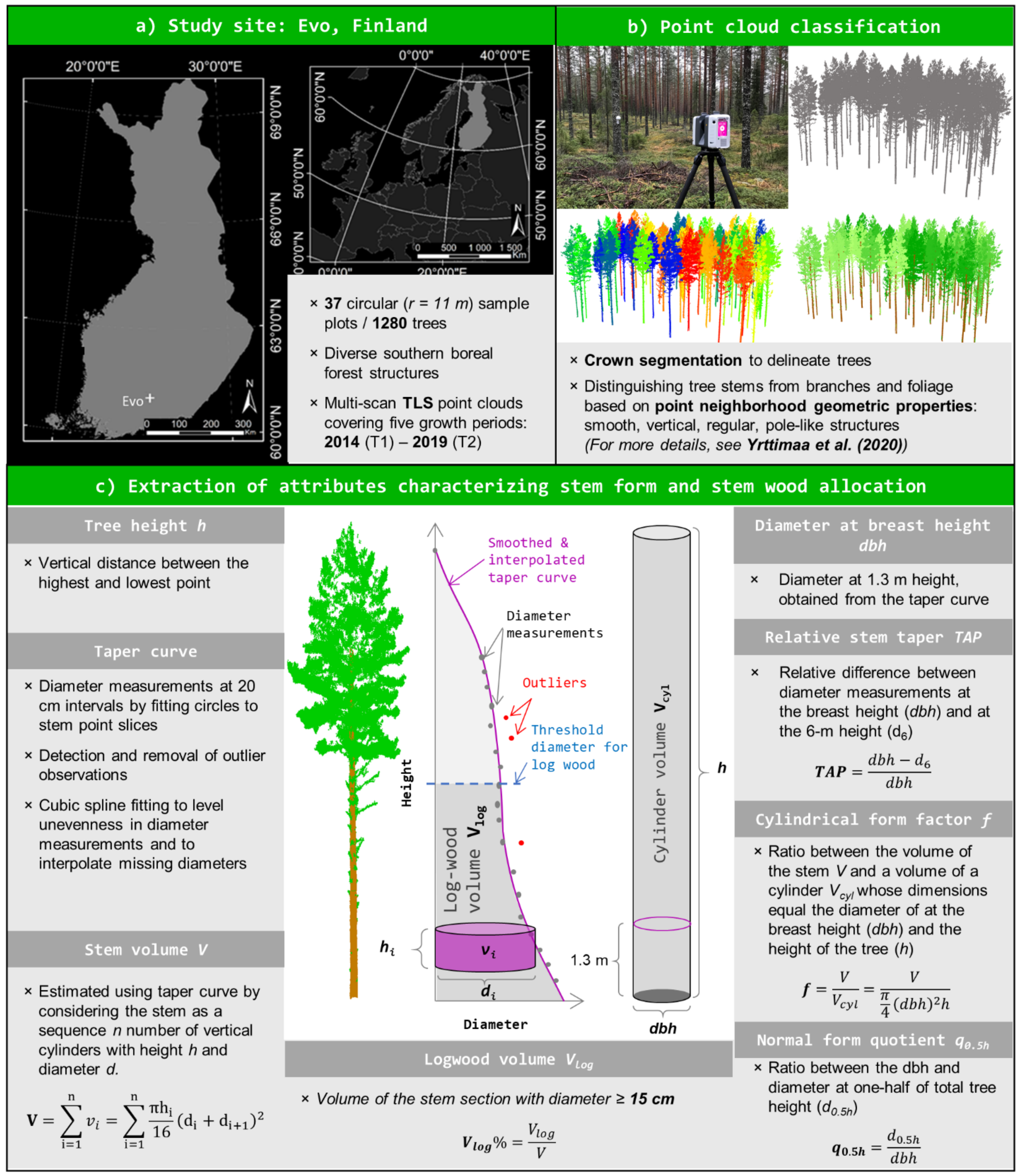
Once the point cloud classification procedure was applied to all trees, the stem points of each tree were used to estimate the taper curve following the methodology presented in [43] and [51]. This involved estimating diameters at 20 cm intervals along the stem by fitting circles and cylinders into stem point slices, detecting potential outlier observations and fitting a cubic spline curve to the diameter-height observations to level unevenness and to interpolate missing observations especially in the upper parts of the stem. Dbh was obtained from the taper curve at the height of 1.3 m above the ground. Stem volume (V) was estimated by considering the stem as a sum of the volumes of vertical cylinders whose dimensions were obtained from the taper curve (see Figure 1).
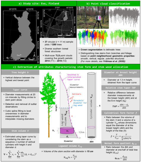
Figure 1.
Description of the study site location as well as the point cloud processing methods used to derive attributes characterizing stem form and stem wood allocation.
Changes in the stem form were quantified with attributes that characterize changes in the relative stem taper (TAP), cylindrical form factor (f), and normal form quotient (q0.5h) (Figure 1c). TAP refers to the relative diameter difference between two predefined stem heights and is usually measured as the relative difference between dbh and diameter measured at the height of 6 m (d6, a.k.a. upper diameter). The f indicates the ratio between V and the volume of a cylinder (Vcyl) whose height and basal area equal to tree height and basal area at the breast height, while q0.5h describes the ratio between the diameter measured at the midpoint (i.e., at the height that equals 50% of the tree height) of the stem (d0.5h) and dbh. Point cloud-based estimates for TAP, f, and q0.5h were obtained at both time points, and their changes (ΔTAP, Δf, and Δq0.5h) were quantified by subtracting the attributes estimated at T1 from the attributes estimated at T2. Increase in TAP and decrease in q0.5h indicate that dbh has grown more than d6 and d0.5h, respectively, which can be interpreted that relatively more stem wood is allocated to the stem base. Changes in TAP and q0.5h are interrelated with changes in the stem form: if more stem wood is allocated to the stem base, the stem form approaches the form of a cone instead of a cylinder, and the values for f decrease.
Changes in the stem wood allocation were quantified in more detail with attributes that characterize changes in V and logwood volume (Vlog). The Vlog was estimated as the volume of the stem section with diameter ≥15 cm using the taper curve. Compared to V, the Vlog is expected to be less prone to uncertainties in the point cloud-based tree measurements as it represents the bottom section of the stem (see Figure 1) which is usually more directly visible to the scanner than the upper part of the stem that often remain occluded by branches [30,40]. Proportion of Vlog to V was computed to obtain logwood volume percentage (Vlog%) which was used to be able to compare stem wood allocation between different-sized trees. The point cloud-based estimates for V, Vlog, and Vlog% were obtained at both time points. To make the change in V and Vlog comparable between different sized trees, relative stem volume increment (ΔV) and relative logwood volume increment (ΔVlog) were used in the analyses of this study. Relative increments were determined by subtracting the attributes estimated at T1 from the attributes estimated at T2 and dividing the result of subtraction with estimated attributes at T1. The change in logwood percentage (ΔVlog%) was quantified in percentage points by subtracting the attributes estimated at T1 from the attributes estimated at T2.
2.4. Methods to Analyze Changes in the Stem Form and Volume Allocation in Different Forest Conditions
The 37 sample plots were divided into four groups representing different forest structures to analyze changes in the stem form and volume allocation in different forest conditions (see Table 2, Figure 2). The classification was based on the average tree size, the development phase and management status of the forest stand. The first group consisted of 268 trees on 8 sample plots that represented young and managed, even-aged, and single-layered forest stands with sparse understory, hereafter denoted as ’young-managed’ sample plots. In this group, basal area-weighted mean diameter (Dg) and -height (Hg) and mean basal area (G) ranged between 15.1–23.6 cm, 13.7–21.6 m, and 17.2–38.6 m2/ha, respectively, and most of the trees were at a rapid growth stage. On average, an increase of 1.3 cm (8.1%) in dbh and 1.6 m (9.7%) in tree height were recorded for the total number of 219 trees that were detected from the point clouds at both time points. The dbh distribution characterizing the tree size variation within the sample plots of this group was unimodal (Figure 2a), which is typical for managed forest stands where silvicultural activities have aimed at allocating the growth to the largest trees of a forest stand, e.g., [57].
Table 2.
Variation of field-measured forest structural attributes such as basal area-weighted mean diameter (Dg) and -height (Hg), mean basal area (G), the number of trees per hectare (TPH), and mean volume (Vmean) which were aggregated from the tree attributes at the sample plot level, as well as the bias and root mean square error (RMSE) of terrestrial laser scanning (TLS) point cloud-derived estimates for diameter at breast height (dbh) and tree height (h) for each forest structural group at the end of the monitoring period (2019, T2).
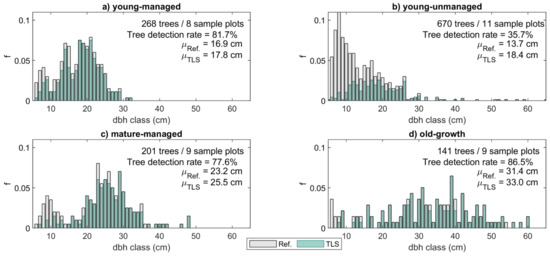
Figure 2.
Diameter at breast height (dbh) distributions for each forest structural group. The bars represent the relative frequency (f) of trees in each dbh class based on field measurements (Ref.) with dark coloring referring to the proportion of trees that could be detected from the terrestrial laser scanning (TLS) point clouds both at the beginning and at the end of the monitoring period. For comparison, the mean dbh values (μ) for the field-measured and TLS-derived trees are provided for each forest stand class alongside the number of trees and sample plots as well as the overall tree detection rate.
The second group consisted of 670 trees on 11 sample plots that represented unmanaged, multi-layered, and mixed-species forest stands with dense understory of young trees competing from growth resources. This group is hereafter denoted as ‘young-unmanaged’. More variation in the forest structural attributes was recorded among the sample plots of this group compared to the other groups (Table 2). There, Dg, Hg, and G ranged between 14.3–43.2 cm, 17.3–27.8 m, and 31.2–56.8 m2/ha, respectively. The reverse J shape of the dbh distribution characterizing the tree size variation within the sample plots of this group was typical for unmanaged, multi-layered forest stands where the number of small trees is considerably higher than that of large trees (Figure 2b) [57,58]. On average, an increase of 1.2 cm (7.2%) in dbh and 1.6 m (9.0%) in tree height was recorded for the 239 trees that were detected from the point clouds at both time points.
The third group consisted of 201 trees on 9 sample plots that represented mature and managed, mostly even-aged, and single-layered forest stands with some undergrowth trees. In this group, hereafter denoted as ‘mature-managed’, the trees were larger in size with growth rate steadily slowing compared to trees in the previous groups. There, Dg, Hg, and G ranged between 24.2–36.8 cm, 22.0–27.0 m, and 20.5–49.2 m2/ha, respectively (Table 2). The dbh distribution characterizing tree size variation within the sample plots of this group was bimodal (Figure 2c) indicating that the next generation of trees was already growing under the dominant tree layer. Out of the 201 field-measured trees, a total of 156 trees (77.6%) were detected from the point clouds at both time points (Figure 2c), and an average increase of 1.2 cm (4.9%) in dbh and 1.1 m (4.8%) in tree height was recorded for these trees.
The fourth group consisted of 141 trees on 9 sample plots representing old-growth Norway spruce-dominated forest stands with relatively sparse understory, hereafter denoted as ‘old-growth’ sample plots. As the name implies, the growth rate of the largest trees in this group had continued to decrease, and an average increase of 0.8 cm (2.6%) in dbh and 1.2 m (4.7%) in tree height was recorded for these trees. The field-measured estimates for Dg, Hg, and G ranged between 35.6–44.0 cm, 27.5–32.4 m, and 35.4–53.8 m2/ha, respectively (Table 2), and the dbh distribution showed that the sample plots enclosed large tree size variation (Figure 2d). A total of 122 trees (86.5%) were detected from the point clouds at both time points (Figure 2d).
Analyses on the changes in the stem form and volume allocation were based on 736 trees for which the point cloud-based estimates for ΔTAP, Δf, Δq0.5h, ΔV, ΔVlog, and ΔVlog% could be extracted; in other words, the stem could be characterized at both time points. This means that out of the total number of 1280 field-measured trees, 544 trees were left outside the analyses due to incomplete tree detection at T1 and/or T2. Most of these trees were small in size and belonged to young-unmanaged sample plots (see Figure 2) that were characterized by complex forest structure, which has been confirmed to affect the performance of the point cloud-based forest characterization [51,53]. Performance in tree detection (tree detection rate of 77.6–86.5%) and the accuracy of the point cloud-derived estimates for tree attributes such as dbh (root-mean-square-error, RMSE of 2.5–3.2%) and tree height (RMSE 8.4–11.2%) were somewhat consistent among young-managed, mature-managed, and old-growth forests where the population of point cloud-derived trees corresponded well to the population of field-measured trees (Table 1, Figure 2). Instead, in the case of young-unmanaged sample plots, a significantly decreased performance in detecting trees (tree detection rate of 35.7%) and estimating dbh (RMSE 6.1%) and tree height (RMSE 28.4%) was obtained using the point cloud-based method.
Paired-sample t-tests were used to analyze whether the point cloud derived estimates for TAP, f, q0.5h, V, Vlog, and Vlog% at T1 significantly differed from the respective estimates at T2, in other words, whether a change in the stem form or volume allocation had occurred during the monitoring period. The H0 in paired sample t-tests for the whole data and on the group-level was: “There is no significant difference between the values of the attribute in question in time points T1 and T2”. The alternative hypothesis for V, Vlog was: “The value of the attribute in question has increased significantly from T1 to T2” and for Vlog%, TAP, f, q0.5h: “The value of the attribute in question has either increased or decreased significantly from T1 to T2”.
Two-sample t-tests were used to analyze whether there were differences in the changes in stem form (ΔTAP, Δf, Δq0.5h) and volume allocation (ΔV, ΔVlog, and ΔVlog%) between different forest conditions, in other words, young-managed, young-unmanaged, mature-managed, and old-growth forests. Then, it was also analyzed how much was the variation in the point cloud-derived estimates for ΔTAP, Δf, Δq0.5h, ΔV, ΔVlog, and ΔVlog% between trees on similar forest conditions (i.e., within each group) and between trees from different forest conditions (i.e., between groups). The respective H0 in two-sample t-tests between the forest structural groups was: “There was no significant difference in the change of the attribute in question between groups X and Y during the monitoring period”, whereas the alternative hypothesis was formed as: “There was a significant difference in the change of the attribute in question between groups X and Y during the monitoring period.” For the two-sample t-tests within the groups, H0 was: “There was no significant difference in the change of the attribute in question between plots A and B during the monitoring period”, and the alternative hypothesis was: “There was a significant difference in the change of the attribute in question between plots A and B during the monitoring period”.
3. Results
3.1. Changes in the Stem Form
3.1.1. Overall Changes
Paired-sample t-tests showed that the point cloud-derived estimates for TAP, q0.5h, and f at T1 significantly (p < 0.01) differed from the respective estimates derived at T2; this led to rejection of H0 in case of all the three attributes, which indicated that a change in the stem form had occurred during the monitoring period when trees from all the sample plots were considered. On average, TAP was estimated to have decreased by 1.4%-points while f and q0.5h were estimated to have decreased by 0.027 and 0.030, respectively (Table 3).
Table 3.
Means and standard deviations (std.) of the estimated attributes characterizing stem form (i.e., relative tapering (TAP), form quotient (q0.5h) and form factor (f)) at the beginning (2014, T1) and at the end of the monitoring period (2019, T2) as well as their change (Δ) reported for trees in different forest structural groups as well as for all trees used in this study.
3.1.2. Changes within Similar Forest Conditions
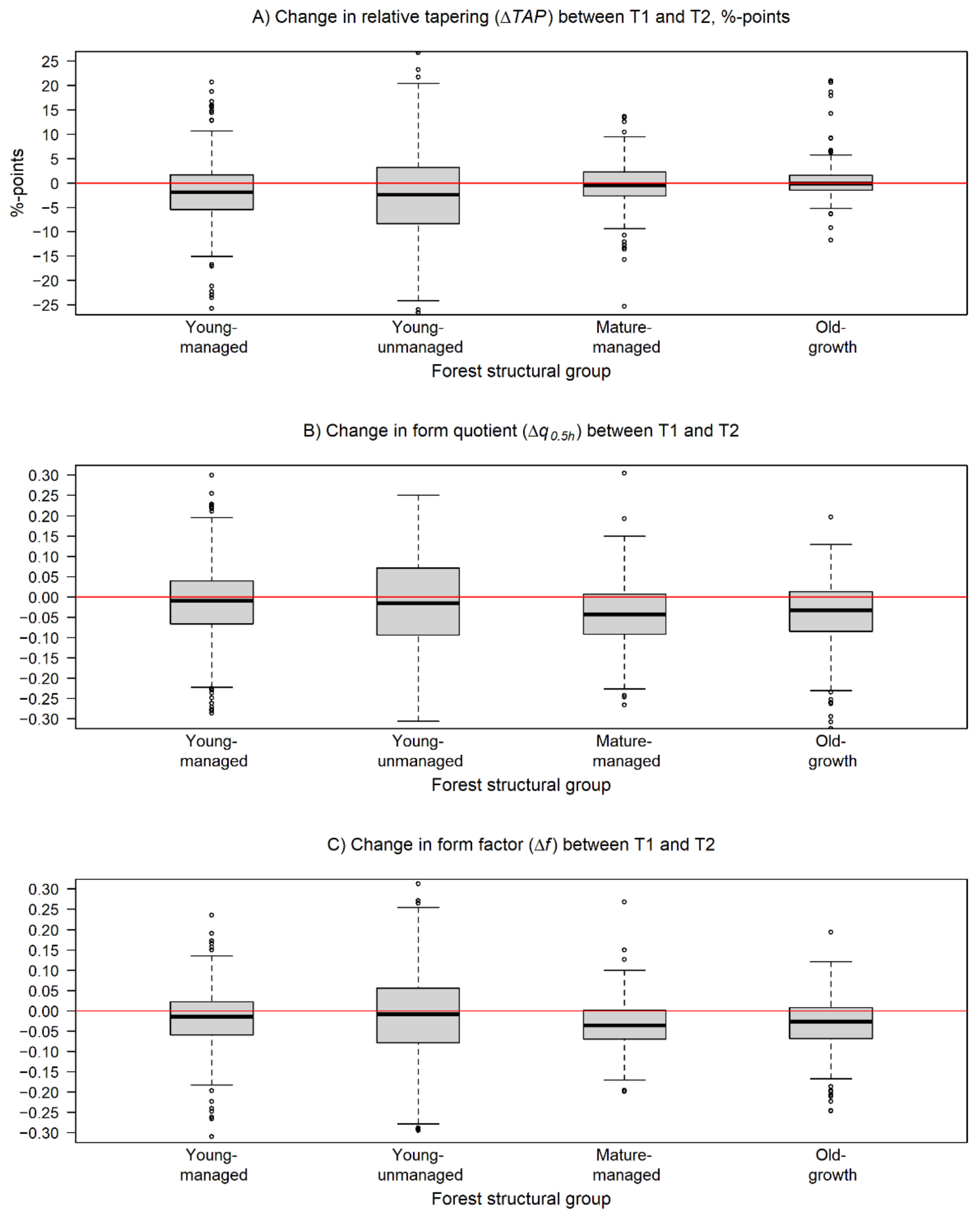
Investigations at the forest structural group level revealed differences in the observed changes in the studied attributes between different forest conditions. Decrease in TAP was recorded for trees in young-managed (−2.3%-points), young-unmanaged (−2.3%-points), and mature-managed forests (−0.5%-points) while an increase was recorded for trees in old-growth forests (0.7%-points). TAP ranged from 12.2% to 21.9% in T1 and from 12.9% to 19.5% in T2 (Table 3, Figure 3A). Paired-sample t-tests showed that the changes in TAP were significant (p < 0.05) only for trees belonging to young-managed and young-unmanaged sample plots.
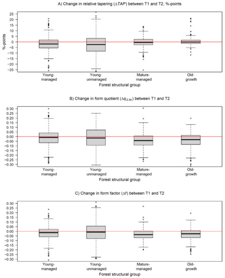
Figure 3.
Box and whiskers plots describing the variation in the changes of the estimated (A) relative stem tapering (ΔTAP), (B) normal form quotient (Δq0.5h), and (C) cylindrical form factor (Δf) during the monitoring period within the forest structural groups. The black line represents the median of the change, and the box borders show the lower and upper quartile of the variation. The whiskers are used to indicate 1.5 times the interquartile range from the upper and lower quartiles. The changes in TAP are presented in percentage points while changes in q0.5h and f are presented in absolute units. The horizontal red line is equal to no change.
The point cloud-derived q0.5h estimates at T1 differed significantly (p < 0.01) from the respective estimates at T2 on young-managed, mature-managed, and old-growth forests. In T1, q0.5h varied from 0.732 to 0.760 and in T2 from 0.698 to 0.726 (Table 3). On average, the change in q0.5h was negative for all groups varying from −0.020 to −0.049 with the change being smallest for trees in young-managed forests and largest in old-growth forests (Table 3).
When examining changes in f, the paired-sample t-tests showed that there was a statistically significant (p < 0.05) change detected during the monitoring period within all forest structural groups. The f varied from 0.520 (mature-managed) to 0.548 (young-unmanaged) in T1 and in T2 from 0.488 to 0.528 for the same groups, respectively (Table 3). Hence, Δf was negative for all groups ranging from −0.019 (young-unmanaged) to −0.041 (old-growth).
Comparisons of the changes in TAP, q0.5h, and f between sample plots within similar forest conditions revealed that the changes in TAP, q0.5h, and f were similar in most of the cases for plots belonging to the same forest structural group. These results indicate that the stem form was developing in the same way within similar forest conditions.
3.1.3. Changes between Different Forest Structural Groups
Comparisons of the changes in TAP, q0.5h, and f between trees within different forest conditions revealed that, in general, the changes were independent of forest structure. Despite the fact that the changes in TAP were detected to be significant (p < 0.05) only within young-managed and young-unmanaged forest, in pairwise comparisons between different forest structural groups, no significant differences (p > 0.05) in ΔTAP were noticed. In addition to this, estimates of TAP were on a higher level for forest structural groups where ΔTAP was detected to be on a significant level. Thus, it seems that the stem form of trees in forests in a younger development phase is developing more towards the form of a cylinder, in other words, the value of d6 is closing on to the value of dbh. While trees in forests in older development phases with already lower values of TAP seemed to allocate more of their growth to the lower parts of the stem to maintain the current level of TAP. In the case of q0.5h and f, however, the observed changes between different forest structural groups were not considered statistically significant (p > 0.05), and thus, the changes in these attributes could be considered similar for all trees regardless of forest conditions (Figure 3B,C).
3.2. Changes in Stem Volume Allocation
3.2.1. Overall Changes
Based on the performed t-tests, all the investigated attributes characterizing stem volume allocation had changed significantly during the monitoring period. The point cloud-derived estimates for V, Vlog, and Vlog% at T1 significantly (p < 0.001) differed from the respective estimates at T2 when all the trees were considered. On average, ΔV and ΔVlog were 25.4% and 67.1% for all the trees in the study, respectively, which shows that the stem volume and the proportion of logwood volume had increased as expected (Table 4). The Vlog% had increased on average of 4.9%-points during the monitoring period.
Table 4.
Means and standard deviations (std.) of the estimated attributes characterizing stem volume allocation at the beginning (2014, T1) and at the end of the monitoring period (2019, T2) as well as their change (Δ) for trees in different forest structural groups as well as for all trees used in this study. Stem volume (V) and logwood volume (Vlog) are reported in m3 whereas logwood percentage (Vkog%) is presented in % in the table. Relative change in stem volume (ΔV) and relative change in logwood volume (ΔVlog) are presented in percentages whereas change in logwood percentage (ΔVlog%) is reported in percentage points.
3.2.2. Changes within Similar Forest Conditions
When investigating changes in the volume allocation within the different forest structural groups, it was noticed that the increase in the point cloud-derived estimates for V and Vlog was statistically significant (p < 0.001) for all the forest structural groups. The V ranged from 0.192 m3 to 1.211 m3 in T1 and from 0.259 m3 to 1.343 m3 in T2 with the respective relative changes in V varying from 10.0% in old-growth forests to 35.3% in young-managed forests (Table 4 and Figure 4A). Similarly, the Vlog ranged from 0.101 m3 to 1.153 m3 in T1 and from 0.162 m3 to 1.280 m3 in T2 with the respective relative change varying from 18.5% to 146.2%. The change in Vlog% was considered statistically significant (p < 0.01) in young-managed, young-unmanaged, and mature-managed forests. The mean Vlog% ranged from 34.0% to 82.7% in T1 and from 43.1% to 83.4% in T2 with the respective change being 0.7–9.1 percentage points (Table 4 and Figure 4B).
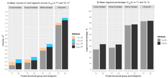
Figure 4.
(A) Mean stem volume and logwood volume of trees in different forest structural groups in T1 and T2. The bars represent the mean stem volume (V, m3) and mean logwood volume (Vlog, m3) in T1 and T2 within forest structural groups young-managed, young-unmanaged, mature-managed, and old-growth, respectively. (B) Mean logwood percentage (Vlog%, %) in T1 and T2 within the forest structural groups used in the study.
Then, it was also further tested whether the changes in V, Vlog, and Vlog% were similar within sample plots belonging to the same forest structural group. In general, the relative changes in the allocation of volume and logwood volume of tree stems remained at the same level within the sample plots belonging to the same forest structural group. Moreover, for ΔVlog%, the changes were similar in most of the cases within the same forest group. This further supports the finding that the volume allocation of trees was mainly similar among the plots within the specific structural group.
3.2.3. Changes between Different Forest Structural Groups
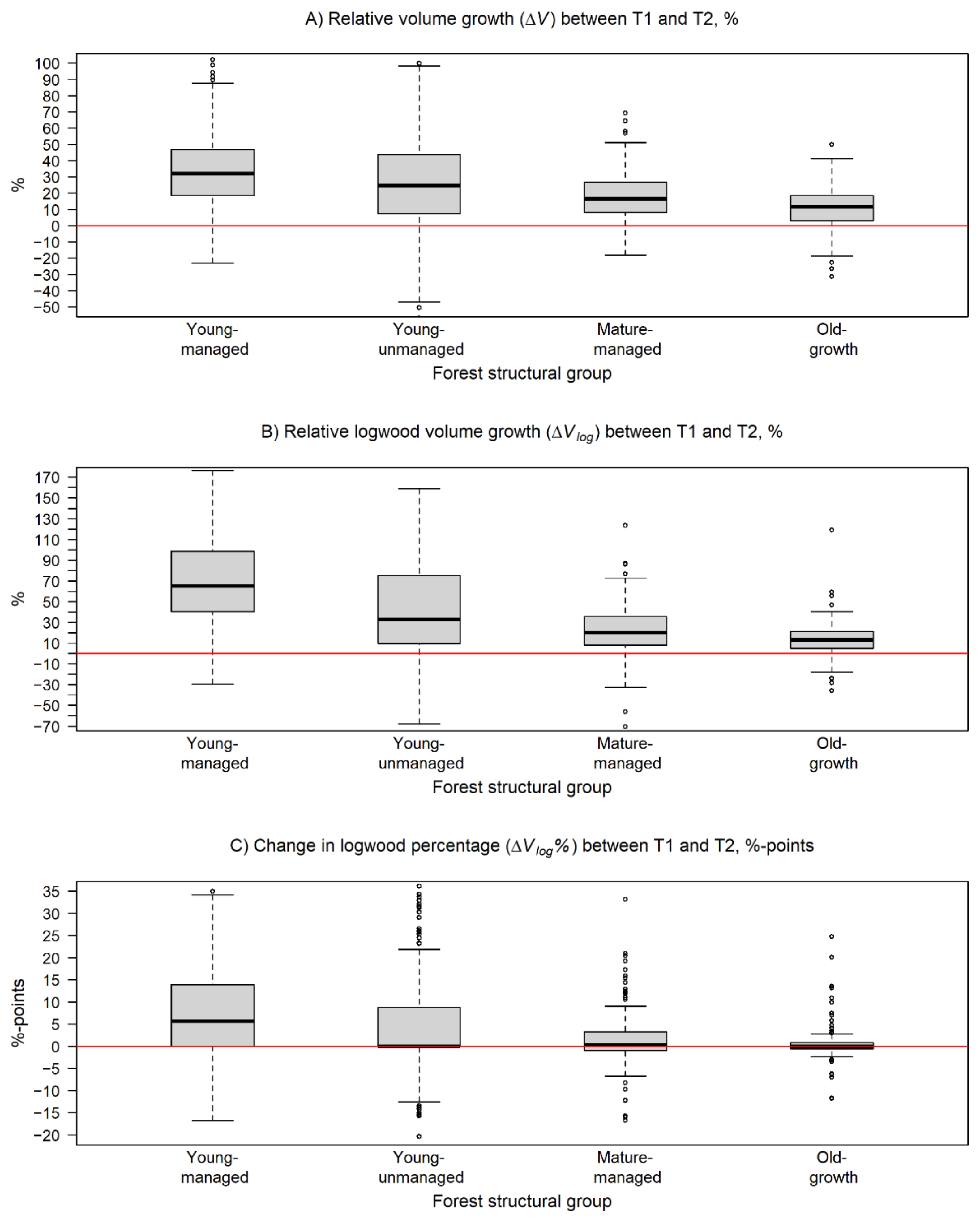
The realized increments in V, Vlog, and Vlog% seemed to vary between the forest structural groups being at a higher level in young-managed and young-unmanaged than in mature-managed and old-growth forests. The ΔV was highest among trees in young-managed forests followed by young-unmanaged, mature-managed, and old-growth forests, respectively (Figure 5A). Two-sample t-tests showed that the respective H0 could be rejected with p < 0.05 in all comparisons between the groups, which means that the relative change in V was significantly dependent on the forest structure.
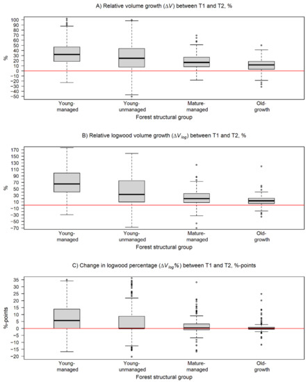
Figure 5.
Box and whiskers plots describing the variation in change of the estimated stem volume attributes within the forest structural groups during the monitoring period. In the plots, the black line represents the median of change and the box borders show the lower and upper quartile of the variation. The whiskers are used to indicate 1.5 times the interquartile range from the upper and lower quartiles. In (A), the relative change in stem volume (ΔV) and, in (B), the relative change in logwood volume (ΔVlog) are presented in percentages. In (C), the change in logwood percentage of tree stems (ΔVlog%) is reported in percentage points. The horizontal red line is equal to no change.
For Vlog, the pairwise comparisons showed a significant difference (p < 0.001) in ΔVlog between trees in young-managed and mature-managed forests as well as between trees in young-managed and old-growth forests, respectively. ΔVlog was most intensive in young-managed (146.2%) and young-unmanaged (76.5%) forests in contrast to the respective changes of 23.5% and 18.5% in mature-managed and old-growth forests (Table 4, Figure 5B). This means that, on average, ΔVlog was on a significantly higher level among trees in young-managed forests compared to trees in mature-managed or old-growth forests.
The pairwise comparisons between forest structural groups showed that there was a significant difference (p < 0.001) in ΔVlog% in all other comparisons except for the comparison between mature-managed and old-growth forest. These two groups also had the smallest increase in Vlog% with 1.6 and 0.7 percentage points, respectively, whereas an increase of 9.1 and 5.4 percentage points was recorded for trees in young-managed and young-unmanaged forests, respectively (Table 4, Figure 5C). These findings can be interpreted that the trees belonging to the old-growth forests are already close to reaching their maximal level of Vlog%.
4. Discussion
The main objective of this study was to investigate the feasibility of using two-date TLS point clouds in examining changes in the stem form and volume allocation in diverse boreal forest conditions. A total of 736 trees from 37 sample plots were characterized with point clouds at the beginning and at the end of the five-year monitoring period. The results showed that the trees were grown in stem volume, and the proportion of logwood volume was increased (see Figure 4), as expected based on earlier findings reported by e.g., [25]. According to our investigations, the stem form had changed, and on average, the stem shape was slightly approaching the form of a cone instead of a cylinder. This implied that the trees tended to allocate more stem wood to the lower parts of the stem. Then, the experimental design of this study enabled analyzing changes in tree growth in different forest structural conditions. For this task, the sample plots were divided into four forest structural groups that represented different growing conditions (see Table 2 and Figure 2). Pairwise comparisons within and between the groups revealed that at the whole tree level the changes in the stem form were similar regardless of the forest structure. Although an increase in V and Vlog was recorded for trees in all the forest structural groups, the relative increment of Vlog was at the same level among trees in young-managed and young-unmanaged forests as well as among trees in mature-managed and old-growth forest (see Figure 5). The growth rate of V and Vlog was noticed to be at a higher level in young-managed and young-unmanaged forests, followed by mature-managed and old-growth forests. Altogether, these findings were in line with the current understanding of how trees allocate their growth, which supported the hypothesis of this study that changes in the stem form and volume allocation can be observed with two-date TLS point clouds.
Performance of the point cloud processing method used in this study to extract attributes characterizing stem form and volume allocation was validated in [49,51]. The conclusion of the studies was that the forest structure is the most important factor affecting the accuracy of the point cloud-based method. This was also visible in this study. The accuracy of estimating dbh and tree height (see Table 2) was somewhat uniform on sample plots of young-managed, mature-managed and old-growth forests, whereas the accuracy was on a lower level on sample plots of young-unmanaged forests, which were structurally different to the other groups (see Figure 2). On average, the accuracy of point cloud-based estimates for dbh (RMSE ~0.9 cm at T2) was, however, considered accurate regardless of forest structure (see, e.g., [31]). In this respect, it is expected that the level of accuracy of the point cloud-derived estimates for diameter measurements along the stem is to a large extent on the same level of accuracy with the point cloud-derived dbh estimates. Thus, it is expected to be relevant to compare differences in the changes of TAP, q0.5h, and Vlog between the forest structural groups, as the accuracy of these attributes is largely dependent on the accuracy of diameter estimates. On the other hand, the accuracy of point cloud-derived estimates of f, V, and Vlog% is partly influenced by the accuracy of point cloud-derived tree height estimates, which is a more challenging attribute to be derived from TLS point cloud data (see, e.g., [30,31,59]). The accuracy of point cloud-derived estimates for tree height varied more with forest structure (RMSE 1.7–5.4 m) which may explain some of the variation in the estimates of Δf, ΔV, and ΔVlog% between trees from different forest structural groups.
Related to the performance of the point cloud-based approach, the incapability of the method to detect all the trees from all the sample plots somewhat limited the analyses of the possible differences in stem form and volume allocation between forest structural groups. As expected, the tree detection rate on sample plots belonging to the group of young-unmanaged forests was clearly lower (35.7%) than on sample plots belonging to the other groups (77.6–86.5%) with most of the undetected trees being small in size. This resulted in the fact that the populations of trees that were characterized from point clouds were, to a large extent, similar between young-managed and young-unmanaged forests (see Figure 2). In both groups, the characterized trees were mainly the largest ones and thus expected to have the best growing conditions. In this regard, it is obvious that changes between trees in young-managed and young-unmanaged forests were found similar in this study. On the other hand, this finding is supported by the earlier studies regarding tree growth stating that, irrespective of stand density, the age and size as well as the competitive status of a tree determine its growth rate [13,14,16].
Differences in the changes of stem form and volume allocation between trees in young-managed and mature-managed forests as well as trees in young-managed and old-growth forests are explained by the age of the trees through the development phases of the forest stands. According to the field measurements, the trees were smaller in size in the younger forests than in the mature and old-growth forests (see Table 1 and Figure 2). With a larger stem diameter, the diameter increment tends to decrease because the stem girth increases; in other words, more wood is needed just to add one more layer of cells to xylem. Thus, it is evident that with the same level of diameter-increment, a larger tree accumulates more volume than a smaller tree. This justifies why the growth rate of trees was the highest in young-managed forests, where the dbh was noticed to increase by 9.7% during the monitoring period, followed by trees in young-unmanaged (7.2%), mature-managed (4.9%), and old-growth forests (2.6%). The smaller the tree is, the higher is the relative growth, although in absolute terms, the tree growth, measured as an increment in stem volume, for example, may remain at a lower level for young and small trees than for old and large trees (see Table 4). According to the results of this study, the same seems to apply with logwood volume, whose relative amount increases noticeably once the stem diameter reaches the minimum requirement set for logwood before saturating at a later point (e.g., [25]). Considering the obtained results here, in young-managed and young-unmanaged forests, the proportion of logwood from the total stem volume of the trees was at a seemingly lower level in T1 than in mature-managed and old-growth forests, and thus, even a minimal increment in absolute amount of logwood will lead to a substantial relative increase during the monitoring period (Table 4 and Figure 5). Considering changes in the stem form, it was noticed that more stem wood was allocated at the lower parts of the stem although the observed changes were small (Figure 3), and no significant differences between the different forest structural groups were noticed. However, this was somewhat expected based on experience gained from [48], where small changes in stem form were observed during a nine-year monitoring period. In [48], TAP was noticed to slightly decrease while q0.5h increased, and no statistically significant differences were recorded for f, which are partially contradictory to the findings of this study. However, it needs to be pointed out that the sample size in [48] was considerably lower and field measured tree height as well as different methods for deriving the attributes from point clouds were used. Altogether, the results obtained in this study regarding how trees allocate their growth are logical, and thus, the differences in the growth of trees between different forest structural groups are justified. On the other hand, the findings confirm the investigated hypothesis stating that the changes in the stem form and volume allocation among trees in different forest conditions can be observed with two-date point clouds.
The feasibility of using TAP, q0.5h, and f to characterize stem form is two-folded. When based on traditional field measurements with calipers and clinometers, the use of attributes that can be observed and modelled through a couple of diameters and tree height is justified. However, the results of this study showed that different conclusions can be drawn based on how the stem form has evolved, as the studied attributes characterize slightly different aspects of the stem form. By definition, TAP measures how much the stem tapers between 1.3 and 6 m, and as the heights are fixed at certain heights, their relative height along the stem changes over time, which can lead to inconsistencies especially in monitoring studies [19]. Therefore, observing stem taper using diameter measurements from relative heights along the stem would be more suitable for detecting changes in stem form (e.g., [60]). From a forest management and timber production point of view, however, TAP indicates the characteristics of the most valuable first log [19]. The findings of this study, related to potential inconsistencies in interpretation of the attributes currently used to describe the stem form, may give further support to the need to improve and develop new measurement methods and attributes. Following the example of [61], it could be possible to use the TLS-based point clouds and taper curves derived from them efficiently in providing new attributes and more exact information on the changes in stem form, either on their own or together with the attributes now in use. However, additional studies are still needed to determine which could be the best-fit attributes to be derived from the taper curves to improve the understanding and monitoring of the changes in stem form of trees.
Compared to the use of conventional forest mensuration tools, the point cloud-based methods enable detailed characterization of the 3D structure of trees (e.g., [29,30,35,39]) and their change in time [49]. The results of this study demonstrated that the point cloud-based methods can be successfully utilized also in detecting changes in the stem form and volume allocation of trees, and the validity of the findings were confirmed in different forest conditions. In general, tree growth reflects the availability of growth resources and competition between trees [4,5,6,7,8]. A tree that is capable of allocating growth to its supporting structures, in other words, increasing stem girth and stem wood volume in general, is considered to have adapted its growth strategies to the environment [6,9,10]. In this respect, the capacity of a tree to allocate growth to the lowest part of the stem, in particular, indicates the vitality and ecological status of a tree within a tree community and as a part of a forest ecosystem. This justifies the need to develop point cloud-based methods to monitor changes in the structure of trees and tree communities, which is especially important considering their potential in revealing the physio-ecological processes related to tree and forest growth. In contrast to many of the conventional methods, the use of point cloud technology provides all the information related to tree structure repeatedly and non-destructively, allowing one to obtain tree observations that have previously been unreachable, for example, for ecological follow-up studies.
5. Conclusions
This study aimed at improving the understanding of the use of two-date terrestrial point clouds in observing tree growth in boreal forest conditions, and the investigations were focused on examining changes in stem form and volume allocation during the five-year monitoring period. The main finding of this study was that the point cloud-based method could detect changes in the attributes that characterized stem form and volume allocation, and the observed changes were in line with the current knowledge of how trees allocate their grow. The point cloud-derived attributes at T1 significantly differed from the respective attributes derived at T2. Changes in the attributes characterizing stem form were relatively small although still revealing that, on average, the trees tended to allocate more of the growth to the lower parts of the stem. Further investigations in the changes between trees within and between different forest structural conditions revealed that the point cloud-based method could detect environment-induced differences in the tree growth. In most cases, the growth of trees within similar forest structural conditions was more similar than the growth of trees within different forest structural conditions. Changes in the relative stem taper as well as in the relative increments in total stem volume and logwood volume were more prominent among trees of younger development phases compared with trees in mature and old-growth forests where the relative growth rate of trees was saturated, as expected.
Altogether, the major contribution of this study was that the findings demonstrated the feasibility of using point cloud-based methods to observe changes in tree stem characteristics. The point cloud-based method enables non-destructive approaches for observations of living organisms, which is preferred in monitoring applications. The validity of the findings was supported by the experimental design of this study that consisted of a total of 736 trees characterized with two-date point clouds on 37 sample plots encompassing diverse southern boreal forest conditions. The findings of this study are expected to advance the state-of-the-art in point cloud-based forest monitoring and promote the applicability of point cloud-based approaches as an observation method in ecological studies as well.
Author Contributions
Conceptualization, M.V., N.S., V.K., M.H., H.K., T.Y., and V.L.; methodology, T.Y., V.L., V.K., and N.S.; formal analysis, V.L. and T.Y.; investigation, V.L., T.Y., J.P., and V.K.; resources, M.V., M.H., H.K., A.K., and J.H.; writing—original draft preparation, V.L., T.Y., N.S., J.P., V.K., and A.K.; writing—review and editing, all authors; supervision, M.H. and M.V.; project administration, M.V. and M.H.; funding acquisition, M.V., J.H., M.H., A.K., and V.L. All authors have read and agreed to the published version of the manuscript.
Funding
This research was funded with a grant by the Finnish Cultural Foundation as well as by the Academy of Finland, grant numbers 315079, 345166, 331711, 334001, 337810, and 337127.
Acknowledgments
The authors would like to thank Häme University of Applied Sciences for supporting the research activities in Evo. Open access funding provided by University of Helsinki.
Conflicts of Interest
The authors declare no conflict of interest.
References
- Harris, N.L.; Gibbs, D.A.; Baccini, A.; Birdsey, R.A.; de Bruin, S.; Farina, M.; Fatoyinbo, L.; Hansen, M.C.; Herold, M.; Houghton, R.A.; et al. Global maps of twenty-first century forest carbon fluxes. Nat. Clim. Chang. 2021, 11. [Google Scholar] [CrossRef]
- Sutherland, W.J.; Freckleton, R.P.; Godfray, H.C.J.; Beissinger, S.R.; Benton, T.; Cameron, D.D.; Carmel, Y.; Coomes, D.A.; Coulson, T.; Emmerson, M.C. Identification of 100 fundamental ecological questions. J. Ecol. 2013, 101, 58–67. [Google Scholar] [CrossRef]
- Pretzsch, H. Forest dynamics, growth, and yield. In Forest Dynamics, Growth and Yield; Springer: Berlin Heidelberg, Germany, 2009; pp. 1–39. [Google Scholar]
- Tomé, M.; Burkhart, H.E. Distance-dependent competition measures for predicting growth of individual trees. For. Sci. 1989, 35, 816–831. [Google Scholar]
- Ericsson, T.; Rytter, L.; Vapaavuori, E. Physiology of carbon allocation in trees. Biomass Bioenerg. 1996, 11, 115–127. [Google Scholar] [CrossRef]
- Oliver, C.D.; Larson, B.C. Forest Stand Dynamics: Updated Edition; John Wiley and Sons: Hoboken, NJ, USA, 1996. [Google Scholar]
- Poorter, H.; Nagel, O. The role of biomass allocation in the growth response of plants to different levels of light, CO2, nutrients and water: A quantitative review. Funct. Plant Biol. 2000, 27, 1191. [Google Scholar] [CrossRef] [Green Version]
- Craine, J.M. Reconciling plant strategy theories of Grime and Tilman. J. Ecol. 2005, 93, 1041–1052. [Google Scholar] [CrossRef]
- Bartholome, J.; Salmon, F.; Vigneron, P.; Bouvet, J.M.; Plomion, C.; Gion, J.M. Plasticity of primary and secondary growth dynamics in Eucalyptus hybrids: A quantitative genetics and QTL mapping perspective. BMC Plant Biol. 2013, 13, 120. [Google Scholar] [CrossRef] [Green Version]
- King, D.A.; Davies, S.J.; Noor, N.S.M. Growth and mortality are related to adult tree size in a Malaysian mixed dipterocarp forest. For. Ecol. Manag. 2006, 223, 152–158. [Google Scholar] [CrossRef]
- Weiskittel, A.R.; Hann, D.W.; Kershaw, J.A., Jr.; Vanclay, J.K. Forest Growth and Yield Modeling; John Wiley & Sons: Hoboken, NJ, USA, 2011. [Google Scholar]
- Vuokila, Y. On growth and its variations in thinned and unthinned Scots Pine stands. Metsat. Tutk. Julk. 1960, 52, 1–38. [Google Scholar]
- Larson, P.R. Stem form development of forest trees. For. Sci. 1963, 9, a0001–a0042. [Google Scholar] [CrossRef]
- Kozlowski, T.T. Cambial Growth, Root Growth, and Reproductive Growth; Academic Press: New York, USA, 1971. [Google Scholar]
- Muhairwe, C.K. Tree form and taper variation over time for interior lodgepole pine. Can. J. For. Res. 1994, 24, 1904–1913. [Google Scholar] [CrossRef]
- Tasissa, G.; Burkhart, H.E. Modeling thinning effects on ring width distribution in loblolly pine (Pinus taeda). Can. J. For. Res. 1997, 27, 1291–1301. [Google Scholar] [CrossRef]
- Peltola, H.; Miina, J.; Rouvinen, I.; Kellomäki, S. Effect of early thinning on the diameter growth distribution along the stem of Scots pine. Silva Fenn. 2002, 36, 813–825. [Google Scholar] [CrossRef] [Green Version]
- Mäkinen, H.; Isomäki, A. Thinning intensity and long-term changes in increment and stem form of Scots pine trees. For. Ecol. Manag. 2004, 203, 21–34. [Google Scholar] [CrossRef]
- Mäkinen, H.; Isomäki, A. Thinning intensity and long-term changes in increment and stem form of Norway spruce trees. For. Ecol. Manag. 2004, 201, 295–309. [Google Scholar] [CrossRef]
- McMahon, T. Size and shape in biology: Elastic criteria impose limits on biological proportions, and consequently on metabolic rates. Science 1973, 179, 1201–1204. [Google Scholar] [CrossRef] [PubMed]
- Bullock, S.H. Developmental patterns of tree dimensions in a neotropical deciduous forest. Biotropica 2000, 32, 42–52. [Google Scholar] [CrossRef]
- Sperry, J.S. Evolution of water transport and xylem structure. Int. J. Plant Sci. 2003, 164, S115–S127. [Google Scholar] [CrossRef] [Green Version]
- Mencuccini, M.; Hölttä, T.; Martinez-Vilalta, J. Comparative criteria for models of the vascular transport systems of tall trees. In Size-and Age-Related Changes in Tree Structure and Function; Springer: Dordrecht, The Netherlands, 2011; pp. 309–339. [Google Scholar]
- Hurmekoski, E.; Jonsson, R.; Korhonen, J.; Janis, J.; Makinen, M.; Leskinen, P.; Hetemaki, L. Diversification of the forest industries: Role of new wood-based products. Can. J. For. Res. 2018, 48, 1417–1432. [Google Scholar] [CrossRef] [Green Version]
- Kershaw, J.A., Jr.; Ducey, M.J.; Beers, T.W.; Husch, B. Forest Mensuration; John Wiley & Sons: Hoboken, NJ, USA, 2016. [Google Scholar]
- Kivinen, V.P.; Uusitalo, J. Applying fuzzy logic to tree bucking control. For. Sci. 2002, 48, 673–684. [Google Scholar]
- Rantala, S. Finnish Forestry Practice and Management; Metsäkustannus: Helsinki, Finland, 2011. [Google Scholar]
- Burkhart, H.E.; Tomé, M. Tree form and stem taper. In Modeling Forest Trees and Stands; Springer: Dordrecht, The Netherlands, 2012; pp. 9–41. [Google Scholar]
- Newnham, G.J.; Armston, J.D.; Calders, K.; Disney, M.I.; Lovell, J.L.; Schaaf, C.B.; Strahler, A.H.; Danson, F.M. Terrestrial laser scanning for plot-scale forest measurement. Curr. For. Rep. 2015, 1, 239–251. [Google Scholar] [CrossRef] [Green Version]
- Liang, X.; Kankare, V.; Hyyppä, J.; Wang, Y.; Kukko, A.; Haggrén, H.; Yu, X.; Kaartinen, H.; Jaakkola, A.; Guan, F. Terrestrial laser scanning in forest inventories. ISPRS J. Photogramm. 2016, 115, 63–77. [Google Scholar] [CrossRef]
- Liang, X.; Hyyppä, J.; Kaartinen, H.; Lehtomäki, M.; Pyörälä, J.; Pfeifer, N.; Holopainen, M.; Brolly, G.; Francesco, P.; Hackenberg, J.; et al. International benchmarking of terrestrial laser scanning approaches for forest inventories. ISPRS J. Photogramm. 2018, 144, 137–179. [Google Scholar] [CrossRef]
- Lovell, J.; Jupp, D.L.; Culvenor, D.; Coops, N. Using airborne and ground-based ranging lidar to measure canopy structure in Australian forests. Can. J. Remote Sens. 2003, 29, 607–622. [Google Scholar] [CrossRef]
- Simonse, M.; Aschoff, T.; Spiecker, H.; Thies, M. Automatic Determination of Forest Inventory Parameters Using Terrestrial Laser Scanning. In Proceedings of the Scandlaser Scientific Workshop on Airborne Laser Scanning of Forests, Umeå, Sweden, 3–4 September 2003; pp. 251–257. [Google Scholar]
- Aschoff, T.; Spiecker, H. Algorithms for the automatic detection of trees in laser scanner data. Int. Arch. Photogramm. Remote Sens. Spat. Inf. Sci. 2004, 36, W2. [Google Scholar]
- Thies, M.; Pfeifer, N.; Winterhalder, D.; Gorte, B.G. Three-dimensional reconstruction of stems for assessment of taper, sweep and lean based on laser scanning of standing trees. Scand. J. For. Res. 2004, 19, 571–581. [Google Scholar] [CrossRef]
- Maas, H.G.; Bienert, A.; Scheller, S.; Keane, E. Automatic forest inventory parameter determination from terrestrial laser scanner data. Int. J. Remote Sens. 2008, 29, 1579–1593. [Google Scholar] [CrossRef]
- Disney, M.I.; Boni Vicari, M.; Burt, A.; Calders, K.; Lewis, S.L.; Raumonen, P.; Wilkes, P. Weighing trees with lasers: Advances, challenges and opportunities. Interface Focus 2018, 8, 20170048. [Google Scholar] [CrossRef] [Green Version]
- Calders, K.; Adams, J.; Armston, J.; Bartholomeus, H.; Bauwens, S.; Bentley, L.P.; Chave, J.; Danson, F.M.; Demol, M.; Disney, M.; et al. Terrestrial laser scanning in forest ecology: Expanding the horizon. Remote Sens. Environ. 2020, 251, ARTN 112102. [Google Scholar] [CrossRef]
- Dassot, M.; Constant, T.; Fournier, M. The use of terrestrial LiDAR technology in forest science: Application fields, benefits and challenges. Ann. For. Sci. 2011, 68, 959–974. [Google Scholar] [CrossRef] [Green Version]
- Liang, X.; Hyyppä, J. Automatic stem mapping by merging several terrestrial laser scans at the feature and decision levels. Sensors 2013, 13, 1614–1634. [Google Scholar] [CrossRef] [PubMed] [Green Version]
- Olofsson, K.; Holmgren, J. Single tree stem profile detection using terrestrial laser scanner data, flatness saliency features and curvature properties. Forests 2016, 7, 207. [Google Scholar] [CrossRef]
- Sun, Y.; Liang, X.; Liang, Z.; Welham, C.; Li, W. Deriving merchantable volume in poplar through a localized tapering function from non-destructive terrestrial laser scanning. Forests 2016, 7, 87. [Google Scholar] [CrossRef]
- Saarinen, N.; Kankare, V.; Vastaranta, M.; Luoma, V.; Pyörälä, J.; Tanhuanpää, T.; Liang, X.; Kaartinen, H.; Kukko, A.; Jaakkola, A. Feasibility of Terrestrial laser scanning for collecting stem volume information from single trees. ISPRS J. Photogramm. 2017, 123, 140–158. [Google Scholar] [CrossRef]
- Pitkänen, T.P.; Raumonen, P.; Kangas, A. Measuring stem diameters with TLS in boreal forests by complementary fitting procedure. ISPRS J. Photogramm. 2019, 147, 294–306. [Google Scholar] [CrossRef]
- Kaasalainen, S.; Krooks, A.; Liski, J.; Raumonen, P.; Kaartinen, H.; Kaasalainen, M.; Puttonen, E.; Anttila, K.; Makipaa, R. Change Detection of Tree Biomass with Terrestrial Laser Scanning and Quantitative Structure Modelling. Remote Sens. 2014, 6, 3906–3922. [Google Scholar] [CrossRef] [Green Version]
- Srinivasan, S.; Popescu, S.C.; Eriksson, M.; Sheridan, R.D.; Ku, N.-W. Multi-temporal terrestrial laser scanning for modeling tree biomass change. For. Ecol. Manag. 2014, 318, 304–317. [Google Scholar] [CrossRef]
- Sheppard, J.; Morhart, C.; Hackenberg, J.; Spiecker, H. Terrestrial laser scanning as a tool for assessing tree growth. Iforest Biogeosci. For. 2017, 10, 172–179. [Google Scholar] [CrossRef]
- Luoma, V.; Saarinen, N.; Kankare, V.; Tanhuanpää, T.; Kaartinen, H.; Kukko, A.; Holopainen, M.; Hyyppä, J.; Vastaranta, M. Examining Changes in Stem Taper and Volume Growth with Two-Date 3D Point Clouds. Forests 2019, 10, 382. [Google Scholar] [CrossRef] [Green Version]
- Yrttimaa, T.; Luoma, V.; Saarinen, N.; Kankare, V.; Junttila, S.; Holopainen, M.; Hyyppä, J.; Vastaranta, M. Structural Changes in Boreal Forests Can Be Quantified Using Terrestrial Laser Scanning. Remote Sens. 2020, 12, 2672. [Google Scholar] [CrossRef]
- Luoma, V.; Saarinen, N.; Wulder, M.A.; White, J.C.; Vastaranta, M.; Holopainen, M.; Hyyppä, J. Assessing precision in conventional field measurements of individual tree attributes. Forests 2017, 8, 38. [Google Scholar] [CrossRef] [Green Version]
- Yrttimaa, T.; Saarinen, N.; Kankare, V.; Liang, X.; Hyyppä, J.; Holopainen, M.; Vastaranta, M. Investigating the feasibility of multi-scan terrestrial laser scanning to characterize tree communities in southern boreal forests. Remote Sens. 2019, 11, 1423. [Google Scholar] [CrossRef] [Green Version]
- Ritter, T.; Schwarz, M.; Tockner, A.; Leisch, F.; Nothdurft, A. Automatic mapping of forest stands based on three-dimensional point clouds derived from terrestrial laser-scanning. Forests 2017, 8, 265. [Google Scholar] [CrossRef]
- Yrttimaa, T.; Saarinen, N.; Kankare, V.; Hynynen, J.; Huuskonen, S.; Holopainen, M.; Hyyppä, J.; Vastaranta, M. Performance of terrestrial laser scanning to characterize managed Scots pine (Pinus sylvestris L.) stands is dependent on forest structural variation. ISPRS J. Photogramm. 2020, 168, 277–287. [Google Scholar] [CrossRef]
- Popescu, S.C.; Wynne, R.H. Seeing the trees in the forest. Photogramm. Eng. Remote Sens. 2004, 70, 589–604. [Google Scholar] [CrossRef] [Green Version]
- Meyer, F.; Beucher, S. Morphological segmentation. J. Vis. Commun. Image Represent. 1990, 1, 21–46. [Google Scholar] [CrossRef]
- Bolles, R.C.; Fischler, M.A. A RANSAC-Based Approach to Model Fitting and Its Application to Finding Cylinders in Range Data. In Proceedings of the 7th International Joint Conference on Artificial Intelligence, Vancouver, BC, Canada, 24–28 August 1981; pp. 637–643. [Google Scholar]
- Maltamo, M.; Kangas, A.; Uuttera, J.; Torniainen, T.; Saramäki, J. Comparison of percentile based prediction methods and the Weibull distribution in describing the diameter distribution of heterogeneous Scots pine stands. For. Ecol. Manag. 2000, 133, 263–274. [Google Scholar] [CrossRef]
- Linder, P.; Elfving, B.; Zackrisson, O. Stand structure and successional trends in virgin boreal forest reserves in Sweden. For. Ecol. Manag. 1997, 98, 17–33. [Google Scholar] [CrossRef]
- Wang, Y.; Lehtomäki, M.; Liang, X.; Pyörälä, J.; Kukko, A.; Jaakkola, A.; Liu, J.; Feng, Z.; Chen, R.; Hyyppä, J. Is field-measured tree height as reliable as believed—A comparison study of tree height estimates from field measurement, airborne laser scanning and terrestrial laser scanning in a boreal forest. ISPRS J. Photogramm. 2019, 147, 132–145. [Google Scholar] [CrossRef]
- Snowdon, P.; Waring, H.D.; Woollons, R.C. Effect of fertilizer and weed control of stem form and average taper in plantation-grown pines. Aust. For. Res. 1981, 11, 209–221. [Google Scholar]
- Saarinen, N.; Kankare, V.; Yrttimaa, T.; Viljanen, N.; Honkavaara, E.; Holopainen, M.; Hyyppä, J.; Huuskonen, S.; Hynynen, J.; Vastaranta, M. Assessing the effects of thinning on stem growth allocation of individual Scots pine trees. For. Ecol. Manag. 2020, 474, 118344. [Google Scholar] [CrossRef]


Publisher’s Note: MDPI stays neutral with regard to jurisdictional claims in published maps and institutional affiliations. |
© 2021 by the authors. Licensee MDPI, Basel, Switzerland. This article is an open access article distributed under the terms and conditions of the Creative Commons Attribution (CC BY) license (https://creativecommons.org/licenses/by/4.0/).