Article

Additionality and Leakage Resulting from PES Implementation? Evidence from the Ecuadorian Amazonia

by
Fernando Gordillo
1,2,*,
Paul Eguiguren
3,4,
Margret Köthke
1,
Rubén Ferrer Velasco
1,4 and
Peter Elsasser
1,*
1
Thünen Institute of International Forestry and Forest Economics, 21031 Hamburg, Germany
2
Graduate School Forest and Agricultural Sciences (GFA), Georg-August-Universität Göttingen, Büsgenweg 5, 37077 Göttingen, Germany
3
Carrera de Ingeniería Forestal, Centro de Investigaciones Tropicales del Ambiente y Biodiversidad, Universidad Nacional de Loja, Loja 110111, Ecuador
4
Institute Ecosystem Dynamics and Forest Management in Mountain Landscapes, TUM School of Life Sciences, Technical University Munich, Hans-Carl-von-Carlowitz-Platz 2, 85354 Freising, Germany
*
Authors to whom correspondence should be addressed.
Forests 2021, 12(7), 906; https://doi.org/10.3390/f12070906
Submission received: 2 June 2021 / Revised: 5 July 2021 / Accepted: 7 July 2021 / Published: 12 July 2021
(This article belongs to the Section Forest Economics, Policy, and Social Science)

Abstract

:
Payments for Environmental Services (PES) are instruments which seem well suited for forest conservation. However, their impact on reducing deforestation might be weakened by negligible additionality and leakage effects; the first refers to the low variation in net deforestation rates even in the absence of PES, and the second refers to the displaced deforestation behavior to other areas not covered by PES. For the case of Ecuador, we examine both issues by assessing the historical deforestation trend of selected PES-enrolled areas and that of their adjacent areas to identify deforestation patterns before and after PES implementation. We analyze the additional effect of PES on reducing deforestation by comparison to a baseline as well as to comparable reference sites at two different spatial scales. We also analyze potential leakage effects of PES by comparing deforestation development in adjacent areas. We show that PES has achieved marginally low conservation impacts in enrolled areas with an average difference in net deforestation rates of 0.02 percent points over a period of 28 years. Overall, PES-enrolled areas depict lower annual net deforestation rates than unenrolled areas, albeit at a negligible rate, and there is also some evidence that deforestation decreased in adjacent areas after PES implementation. Additionally, there exists a statistically significant linear increasing deforestation trend in adjacent areas as distance increases from the PES-enrolled area. Our empirical results, however, raise the suspicion that the choice of PES-enrolled areas might have been influenced by self-selection.

1. Introduction

Payments for Environmental Services (PES), defined as voluntary transactions between service users and service providers upon mutually agreed natural resource management rules [1], are widely applied as policy instruments for forest conservation [2,3]. PES are assumed to be favorable for mitigating climate change, reducing emissions from deforestation and forest degradation, providing incentives for forest conservation, and enhancing the provision of environmental services [4,5,6]. Within the context of unsustainable forest use, their goal is to induce additional incentives for forest conservation [7,8]. Although theoretically sound, their environmental and social outcomes have been scrutinized [9,10], thus accentuating the need to better understand the different settings in which PES are embedded [11,12]. Two particular concerns arise when assessing their effectiveness. The first is a possible lack of additionality: even without any financial incentive, program participants might exhibit the targeted behavior [13,14,15]. Put simply, they would leave their forest intact even without any payments. The second is leakage: individuals might move their deforesting and forest degradation activities to other areas not covered by PES [16,17,18,19]. Several empirical studies have analyzed these concerns and found evidence for their practical relevance. In some cases, additionality from self-enrolled low-pressure areas turned out to be negligible [20,21,22,23]. Empirical evidence exists also on leakage effects (i.e., displaced deforestation) within a PES context [24,25,26].
There exists, therefore, a debate regarding PES effectiveness [27,28,29]. Theoretical considerations [30] indicate that direct payments could be more cost efficient than indirect approaches, thus suggesting that PES instruments could be effective in reducing deforestation [31]; adverse self-selection and moral hazard, however, could weaken their effectiveness. Adverse self-selection arises when service providers volunteer their lowest-value forests which might be under the least threat at the same time, implying that less-threatened forested areas could receive payments for conservation while the most threatened areas receive nothing. Moral hazard arises when service providers take unobservable actions—since contract compliance is costly to monitor—that could help them evade the performance of their obligations [32]. Additionally, some PES instruments do not intendedly provide for a continued flow of data collection and are not designed with the intention of evaluating their effectiveness [29]. Ultimately, the effectiveness of PES instruments in avoiding deforestation remains an empirical issue [29,33]. Existing literature presents mixed evidence as to the extent to which implementing a PES instrument could achieve its intended goals [9,10]. Likewise, evidence-based studies that attest to the effectiveness of a PES instrument are also sparse and often very context specific [23,34,35].
In Ecuador, forest cover declined from about 15 million ha in 1990 to approximately 13 million ha by 2016 [36,37,38]. Forests in Ecuador face two major threats: (1) the complete conversion of forested areas to different land uses, usually for agricultural purposes (i.e., deforestation); and (2) a reduction in the capacity of forests to deliver environmental services mainly due to human-induced activities, such as selective logging (i.e., forest degradation) [39,40]. As a policy measure to address such threats, the Ecuadorian government designed and implemented in 2008 a PES program called Socio Bosque (SBP) [41], which has continued in operation since its beginning. It was introduced in 2008, prioritizing specifically targeted forested areas [42] with the dual objective of forest conservation and poverty alleviation following three main criteria: (1) reducing the deforestation threat, (2) supporting environmental services, and (3) abating poverty. Socio Bosque provides differentiated financial incentives to private individuals and indigenous communities in exchange for mutually agreed forest conservation practices [20]. Regarding the implementation of SBP, there exists suggestive positive evidence on the reduction in deforestation [20,21,23,43,44]. The estimates presented there indicate that implementing SBP in locations across Ecuador achieved its primary goal of reducing deforestation rates in SBP-enrolled areas. The mentioned studies are, however, mainly based upon statistical correlations, leaving aside historical deforestation trends and the non-intended effects of SBP on leakage in adjacent areas. We therefore identified a research gap deserving further scrutiny; this is understanding the leakage effects of SBP implementation on adjacent areas [45,46].
We examine the presence of additionality and leakage by focusing on community-owned SBP-enrolled forests and other areas without SBP enrollment for comparison. The latter are adjacent areas, including a sequence of buffer zones around each SBP area, and additionally, comparable reference sites located farther away. We use historical deforestation data from 1990 to 2018 to analyze average annual net deforestation trends within the considered areas. Departing from this information, we question whether the deforestation trends within SBP areas and their adjacent areas would have been the same as those without the presence of SBP, and whether such trends change after the implementation of SBP. In addition, we address the self-selection issue mentioned above by assessing, for a broadened period of time, areas purposely placed under conservation by their communities. We hypothesize that areas under SBP have lower deforestation rates than their adjacent areas after SBP implementation. We provide findings from an evaluation design using t-tests, effect size, and ANOVA analysis that present evidence for additionality in SBP areas, but also for leakage in adjacent areas.
Our study is structured around two intertwined research questions: (1) Has the implementation of SBP caused additional deforestation reduction (compared to the time period before the implementation, and to comparable nonadjacent reference sites)? (2) Has the implementation of SBP induced leakage into their adjacent areas? As a side question, we ask whether the selection process for SBP areas might have been influenced by self-selection, i.e., whether SBP areas might have been located in areas with lower deforestation pressure compared to adjacent areas. In the following sections, we detail the methodology employed for data gathering and choice of empirical approach. We subsequently present our results with respect to the additionality of SBP and leakage effects in our study sites in the Ecuadorian Amazonia. We then discuss our findings in reference to PES design, their applicability for actual policymaking, and methodological challenges for the analysis of additionality and leakage resulting from PES implementation.

2. Materials and Methods

2.1. Study Sites

Geographic area and study site selection used in this analysis came from a project conducted in Ecuador between Thünen Institute and local partners [43,47,48,49,50]. Selected study sites (see Figure 1) are located in the provinces of Napo, Pastaza, and Orellana. These provinces contain approximately 44% (5.5 Mha) of the total forest area in Ecuador [51]. In these three provinces there is more than 1 Mha of land under SBP, which represents approximately 63% of the total SBP area in Ecuador for 2018 [52].
In order to assess additionality, we compared average annual net deforestation rates from the four SBP-enrolled areas before and after SBP implementation. To assure that changes in deforestation rates in SBP areas can deviate from the deforestation trend in the broader landscape, we additionally considered the development in nonadjacent reference areas without SBP and compared the trends in both types of area. The reference areas are located further away from the SBP areas (nonadjacent), but are still located in comparable landscape contexts. The evaluation of economic tools for forest conservation (i.e., PES) should consider the geographic areas (i.e., landscape) where the instrument is implemented [53,54]. Hence, integrating “the broader social and ecological landscapes in which PES initiatives are embedded” [55] is crucial to assess additionality outcomes. For this purpose, a “landscape approach” following a randomized block design [43] was applied. Following this design, we compared pairs of rectangular 100 km2 landscape sections (here called “tiles”, see Figure 1). Each pair consists of one tile that intersects one of the four SBP areas and another tile that does not contain any SBP area. For assessing leakage, we compare the deforestation development of SBP areas and land surrounding SBP areas, referred to as “buffer zones” [56]. The buffer zones represent a sequence of ten 1 km rings around each SBP area (see Figure 1).

2.2. Empirical Approach

To answer our questions about additionality and leakage effects, we conducted the following series of analyses. First, we assessed the historical trend of deforestation in SBP-enrolled areas (checkered hatching in Figure 1) in four study sites by comparing the development of the deforestation before and after the introduction of SBP. This provides an overview of the historical trend of deforestation and helps in the identification of additionality and self-selection bias in adjacent areas [17]. Second, we turned to the rectangular landscape sections (“tiles”) and assessed the development of deforestation in those four tiles that include a proportion of SBP-enrolled area (rectangles 2, 4, 6, and 8 in Figure 1) to those other four tiles where SBP has not been implemented in any part (rectangles 1, 3, 5, and 7 in Figure 1). Third, we partitioned each tile including an SBP area (rectangles 2, 4, 6, and 8 in Figure 1) into two subareas (i.e., the area under SBP and the area without) and subsequently established if there exist statistical differences in average annual net deforestation rates. Finally, as a fourth step, we widened this perspective by exceeding the limitation of the tiles and compared the deforestation development in SBP areas (checkered hatching in Figure 1) against ten 1 km buffer zones (rings in Figure 1) around the borders of each area to analyze any difference related to distance from the conserved zones. Our hypothesis is that deforestation is lower in SBP areas than in their buffer zones after the implementation of SBP, given that the pressure from deforesting practices relocates from the SBP area to adjacent areas (leakage) and that this pressure is distance dependent. We therefore tested the differences in the average annual net deforestation rates between the buffer zones to determine whether there is a dependency on distance.
For all considered areas and time periods, we conducted the following consecutive steps. First, in order to establish a trend in average annual net deforestation rates over time, we identified through tables and graphs, as a pre-screening, whether a change in average annual net deforestation rates could be observed after SBP was introduced. Second, we employed t-test analysis [57] for statistical differences in average annual net deforestation rates across time periods and study sites; for example, a comparison of the average annual net deforestation rate in one particular study site for two time periods. Third, we assessed the variability associated with the effect of SBP implementation on adjacent areas by means of effect size analysis. Effect size is a scale-free, sample size independent, and easily interpretable standardized metric that conveys the identification of the standardized difference between means (Cohen’s d) [58,59] and is also employed to compare the effectiveness of forest conservation mechanisms [60]. This approach, however, does not fully identify independent land-use patterns for each area since the provided financial incentives restrict deforestation practices only in SBP-enrolled areas. It is therefore also plausible that a change in average annual net deforestation rate could have taken place due to a policy-induced spatial spillover that goes beyond the SBP area [18]. Therefore, an ANOVA analysis was conducted as a fourth step; we tested for leakage in direct adjacent areas by establishing statistical differences in two time periods (i.e., before and after SBP implementation) for SBP areas and their ten 1 km buffer zones.

2.3. Analysis of Additionality: Suitable References

A key concern regarding the assessment of SBP is whether it generates additionality. The challenge present in assessing additionality is the difficulty in attributing the difference in deforestation to the influence of a specific policy instrument, i.e., to separate this instrument’s influence from the influence of other socio-economic developments that have affected deforestation rates over time. A plausible way to assess it is to construct a baseline for comparison; namely, a hypothetical scenario without this policy instrument. The alternative is a comparison to empirically observable references. In our case, there are two kinds of empirical observations that inform about deforestation developments without SBP, and can thus serve as references: one is the historic trend in SBP areas that was observable before the implementation of SBP; the other is a comparison to other areas where SBP has not been implemented until now, including the trend that is observable there. For our analysis, we considered a broadened time frame [61] and used historical deforestation data from 1990 until 2018 that included time periods before and after the implementation of SBP in our study sites [62,63] and tracked changes in deforestation rates in enrolled and non-enrolled areas. In order to allow for the comparison of rates from different time periods we standardized the calculation of annual rates of deforestation, as indicated by Puyravaud [64]. An important clarification is necessary here. Although SBP was formally implemented at a national level in 2008, SBP areas did not enroll in the same year. For the SBP areas of Ahuano, Rukullacta, and Ávila, their starting year was 2009, whereas for Canelos it was 2014. We therefore considered time periods before and after SBP, taking into account their starting dates. In the particular case of Canelos, the time period before SBP refers to 1990 until 2014 and the time period after SBP refers to 2014 until 2018.

2.4. Average Annual Net Change in Forest Area

We collected baseline information from the Ecuadorian Ministry of Environment [37,38], which has produced and openly published national land cover maps for the years 1990, 2000, 2008, 2014, 2016, and 2018. These maps are based on a standardized classification method, which categorizes areas of native forest (among other land cover classes) and uses Landsat and Rapid Eye images and ground truthing data collected through all the Ecuadorian provinces for training and validation. Data obtained from the official source (i.e., Ministry of Environment in Ecuador) assure the reliability and consistency of their use for our calculations, are also employed for national statistics and international reporting, i.e., FAO and IPCCC, and reflect the best source regarding temporal and spatial resolution. Using the land cover maps and the free and open source QGIS3 software [65], we calculated the average annual rates of change of forest cover for the periods (e.g., 1990-2008/14 and 2008/14-2018) and areas of interest following the formula suggested by Puyravaud [64]:
N D R = 1 t 2 t 1   ln A 2 A 1
where NDR is the average annual net change in forest area in percent per year, and A1 and A2 are the forest cover of the area of interest at time t1 and t2, respectively. This formula has the advantage over a direct measure in that it better approximates the average annual percentage for a certain period.

3. Results

3.1. Negligible Change in Deforestation Rate before and after SBP

In order to identify the annual changes in net deforestation rates in SBP areas, we compared their annual net deforestation rates from 1990 until 2018 (see Table 1; note that according to Equation (1) a positive sign indicates gains in forest area, whereas a negative sign indicates forest losses; cf. also [66]). In Figure 1, these results refer to the checkered hatching areas. We observed a reduction in annual net deforestation rates after the implementation of SBP when averaging across all study sites, but the effect was small (i.e., a difference of only 0.02 percent points) and statistically insignificant (p-value = 0.45; Cohen’s d = 0.43). Looking at the individual study sites, three of the four sites showed a positive change after SBP implementation, with Ahuano as the exception.

3.2. Lower Deforestation Rates in Reference Tiles Without SBP

To observe whether deforestation decline is greater in SBP tiles than in (nonadjacent) reference tiles without SBP, we compared how their pattern of deforestation evolved through time. In Figure 1, these results refer to pairs of tiles, i.e., 1 and 2, 3 and 4, 5 and 6, and 7 and 8. We observe that in none of the SBP tiles was there a remarkable change in deforestation rates though time (see Table 2). The reference tiles exhibited larger differences in their net deforestation rates across all time periods; however, these changes occurred in both directions. Overall, annual net deforestation rates in tiles with SBP are lower than in reference tiles without SBP over all time periods—before as well as after the establishment of the program.
We employed t-test and effect size analysis for the individual comparison of the statistical differences between an SBP tile and its respective reference tile. We did not find statistical differences in means for Arajuno–Canelos (Cohen’s d = 0.93). For the remaining pairs, however, we found that their means were all statistically different at 1% with Cohen’s d ranging from 4.00 (in San Jose de Dahuano and Ávila) to 7.93 (in Chontapunta and Ahuano), indicating that deforestation was lower in SBP tiles than in tiles without SBP.

3.3. Low Deforestation Rates in SBP Areas Even before SBP Implementation Indicate Self-Selection

In order to establish whether potential self-selection of the SBP areas in locations of low deforestation pressure is prevalent, we compared net deforestation rates in the SBP and non-SBP subareas within the SBP tiles, before SBP implementation (see Table 3). In Figure 1, these results refer to rectangles 2, 4, 6, and 8.
We found that the SBP subareas in each tile showed no deforestation (Ahuano and Rukullacta) or almost no deforestation (Ávila and Canelos) already before SBP implementation, whereas deforestation rates have always been higher in the respective non-SBP subareas. Taking all four study sites together, the differences between SBP and non-SBP subareas are statistically significant at 5% with Cohen’s d = 2.34. When analyzed individually, a case of particular note is Ávila, which was statistically significant at 1% with Cohen’s d = 7.93.

3.4. Reduced Deforestation in Buffer Zones Surrounding SBP-Enrolled Areas after SBP Implementation

We tested our hypothesis that there is a distance effect in buffer zones around SBP areas in order to control for leakage. In Figure 1, these results refer to the checkered hatching areas and the rings. We observe that our four study sites depict varied deforestation behavior before and after SBP implementation (see Figure 2). In Ahuano, net deforestation rates increased after SBP implementation both in the buffer zones and the SBP area. In all three other sites and their respective buffer zones, the deforestation rates decreased after the SBP implementation. In Rukullacta, the SBP area as well as the buffers up to 7 km of distance showed an increase in forest area after SBP implementation. For Ávila and Canelos, net deforestation rates decreased across all buffers after SBP implementation as well, but to a lesser extent. We individually tested each SBP area along with its ten 1 km buffer zones (see Table A1 in Appendix A) before and after SBP implementation and found that they were all statistically different at 1%, with Cohen’s d ranging from 1.09 to 2.87.
Additionally, we compared the annual deforestation rates before and after SBP implementation (ANOVA as the average over all four sites). In general, we observed that annual deforestation rates increased with distance from each SBP area. In both time periods, there was a linear increasing trend in deforestation beginning from the respective SBP area; deforestation increased as distance from SBP area increased (see Figure 3). When we compared the annual net deforestation rates before and after SBP implementation, in every buffer there was no statistical difference except at 6 km (p-value: 0.0925). Although no statistical difference was found, a reduction in the annual net deforestation rates between 36 and 76% after SBP implementation was found across all buffer zones (see Table A2 in Appendix A).
We also tested whether there exists a correlation between net deforestation rates and distance in the SBP areas and the ten 1 km buffer zones. Before SBP implementation, the results indicate a correlation of −0.7833 (p ≤ 0.01; CI between −0.920 and −0.201), and after SBP implementation, a correlation of −0.7664 (p ≤ 0.01; CI between −0.914 and −0.164). In the absence of more precise data, we also conducted two standard linear regressions with a constant between net deforestation rates and distance. Our interest in the results (see Table 4) from these regressions lay in the coefficient of distance.
Overall, the regression results indicate that distance is statistically significant in explaining net deforestation rates in the SBP areas and buffer zones, before as well as after SBP implementation. Our estimates are stable across both time periods, thus depicting a consistent increase in deforestation in farther buffer zones. Beyond this, we observe that the coefficient of distance decreased after SBP implementation (however, the latter could be a random result, as the confidence intervals of both distance coefficients overlap).

4. Discussion

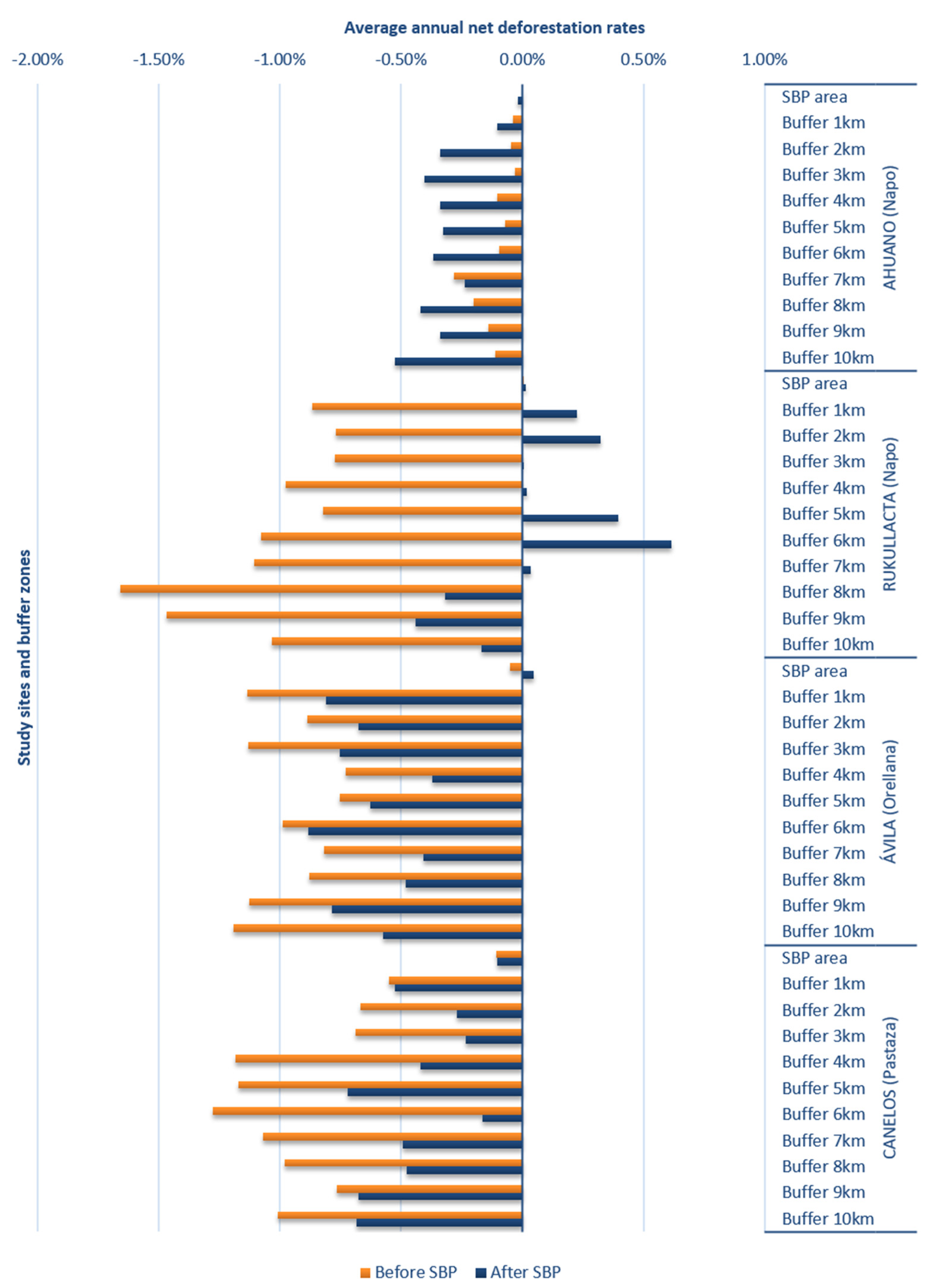
To test the effectiveness of SBP implementation in four Ecuadorian sample sites under the claim of additionality and avoided leakage, we tracked changes in annual net deforestation rates in SBP areas and non-SBP areas, both adjacent to and far away from the study sites; altogether, the analyzed time period was 28 years. The results reveal that the average difference in annual net deforestation rates for SBP areas before and after SBP implementation is marginally low (about 0.02 percent points); however, the overall net deforestation rates in these areas are considerably lower than the nonadjacent reference sites without SBP. Distance to SBP areas is decisive for deforestation intensity, which was shown by a statistically significant linear increasing trend of deforestation departing from SBP areas. Additionally, under the simplifying assumption that effect size estimates accurately represent changes in net deforestation rates, we argue that such changes could be attributed to the implementation of SBP. In analyzing the historical net deforestation trend in SBP and non-SBP areas, it appears as if SBP was mainly introduced in regions where net deforestation was low and stable anyway, while it rose in comparable reference sites and adjacent areas. Currently existing data limitations and methodological challenges for the assessment of additionality and leakage offer, however, scope for interpretation.

4.1. Methodological Issues

We obtained very high estimates of Cohen’s d in the comparison of the tiles located in Chontapunta and Ahuano (Cohen’s d = 7.93) and in SBP vs. non-SBP areas in Ávila (Cohen’s d = 7.93). Although Cohen [67] and Sawilowsky [68] provide a rule of thumb when analyzing estimates for effect sizes ranging from very small (0.01) to huge (2.0), Slavin and Smith [69] indicate that large effect sizes may result from small sample sizes and Börner, Schulz, Wunder, and Pfaff [60] state that differences in dynamic context factors may also reflect variations in estimates. We therefore ask the reader to use caution in interpreting effect size estimates as a clear indication of self-selection, additionality, and leakage but rather as a signal of the differences in outcomes and the practical consequences of SBP implementation [59]. Additionally, results obtained from ANOVA and t-tests indicate a discrepancy in statistical significance; t-tests returned significant differences whereas ANOVA results did not. A plausible reason is that t-tests are not additive whereas ANOVA analysis sums up means to find differences among groups [70]. We argue that there may exist a difference in means when assessed as a group, but due to a high level of noise coming from unaccounted-for contextual factors, such a difference is undetectable in our data. Hence, our individual findings suggest statistical differences, although they do not show it as a group. Such discrepancy indicates that contextual factors and the individual analysis of historical net deforestation trends in SBP areas and comparable reference sites could capture the differences in outcomes when assessing self-selection, additionality, and leakage.

4.2. Additionality and Self-Selection

Additionality of SBP implementation manifests in additionally avoided deforestation in the SBP areas, compared to the counterfactual case. In the absence of true counterfactuals (what would have happened in the absence of SBP in this site?), we made comparisons to diverse reference sites: buffer zones around SBP areas, non-SBP subareas within landscape sections (tiles) that are part of the beforementioned buffer zones, and tiles under comparable conditions far away from the SBP tiles. For all those, deforestation development in time periods before and after the SBP implementation was observed. While the overall effect of deforestation reduction in the SBP areas is marginally low (about 0.02 percent points), deforestation in the considered areas without SBP was higher over the whole time period of 28 years.
In assessing changes in annual net deforestation rates between time periods, we observed the difference before and after SBP implementation. An alternative view involves scrutinizing the changes in the number of hectares in forest areas. Over a period of 28 years, comparable reference sites (tiles) lost on average 25.69% of their forest areas (Chontapunta 29%, Carlos Julio Arosemena Tola 20%, San José de Dahuano 45%, and Arajuno 9%) in comparison with 0.83% of forest area loss in SBP tiles (Ahuano 0.20%, Rukullacta 0.26%, Ávila 0.41%, and Canelos 2.96%). Despite having a relatively low percentage change in deforestation rates, there is indeed some change in terms of forest area. In each case, however, SBP-enrolled areas had a smaller loss of forested areas when compared against several references.
Notable, however, is the fact that the annual net deforestation rates in SBP areas were distinctly lower already before SBP implementation, which questions the presence of deforestation risk in these sites and therefore the additionally effect. The literature indicates that PES’ impact on the abatement of deforestation is low [29]. For the case of Ecuador, our finding of low changes in annual net deforestation avoidance in SBP areas is similar to other empirical work [20,21,22,23,71] using different methodologies (e.g., randomized control trials, score matching). The low annual net deforestation rates in enrolled SBP areas need not be interpreted as SBP being ineffective but rather as possibly exposing a landowner´s decision to assign an area of land into a profitable activity (i.e., conservation under a PES instrument) [72]. From this perspective, landowners might already have been aware of the profitability of conserving forested areas before the existence of SBP, and this awareness prompted them to “secure” these areas by joining SBP once this program was available. Under these circumstances, it seems reasonable to assume that the financial incentives provided by SBP reinforced their desired investment behavior. The pattern of low deforestation in SBP areas and intensified land use in adjacent areas was already present long before SBP was designed or implemented in our study sites. In short, such behavior would have been maintained even in the absence of payments [9,13,25]. It is likely that those proactively secured areas are of lower suitability for other land uses, thus causing comparatively low opportunity costs of forest conservation. The deforestation risk attributed to those areas might therefore be rated as low. Such behavior reveals asymmetric information and flawed spatial targeting that exacerbates the degree of non-compliance and spatial spillovers [32]. It becomes unclear, however, whether SBP implementation is the main factor of influence for avoiding deforestation, absent an initial deforestation risk.
Furthermore, joining SBP implies self-enforcement, since failure to comply with agreed management rules translates into penalties [73]. Additionally, an issue connected to self-enforcement is the number of hectares under conservation agreement for which monetary incentives are provided (an overview of the levels of monetary incentives received by individuals and communities is detailed by [20]). We argue, therefore, that abiding by contract rules prompts communities to maintain compliance at a minimum, receive financial benefits, and maintain a more intense land use in adjacent areas. All in all, this reduces additionality [45].

4.3. Leakage

We observe a change in deforestation rates in SBP areas and adjacent buffer zones after SBP implementation. A comparison of deforestation rates across time periods revealed consistency in deforestation patterns. In the ten km buffer zone around SBP areas, the average net deforestation rate decreased to a higher degree (−0.42%) than in the SBP areas themselves (−0.02%) (see Figure 3 and cf. [49]); an evident decrease in deforestation after SBP implementation over time. Since this change in net deforestation rates for SBP areas between periods is marginally small, it makes it troublesome to attribute the aforementioned change in deforestation behavior to the implementation of SBP. Our finding of higher deforestation rates in buffer zones is, however, similar to the empirical work of Ford et al. [74], conducted in tropical and subtropical regions of America, Africa, and Asia, in which deforestation rates were higher in 10 km buffer zones than in protected and control areas, thus undermining forest conservation efforts.
We detect that forest cover changes (decreases and increases in net deforestation rates) in SBP areas happen in the same direction as in the surrounding areas. For example, Ahuano had the highest deforestation rates in its buffer zones after SBP implementation, which increased over time. In the same direction, Ahuano showed a slight increase in deforestation within the SBP area as well. All other SBP areas showed a decrease in deforestation rates after SBP implementation. This decrease was also observable in the surrounding buffer zones, which maintained, however, a high rate of deforestation. Only in the buffer zones of Rukullacta did reforestation occur after SBP implementation, up to the 7 km buffer zone.
Our results are similar to those reported by Arturo Sánchez-Azofeifa et al. [75] in a study on Costa Rica’s national parks and biological reserves, and buffer zones around them; their results indicate that as distance increases from protected areas (in this case national parks and biological reserves), total deforestation and deforestation rates also increase. There exists, however, the possibility that leakage effects on nearby parcels could be positive or absent, possibly due to differences in pressure, as emphasized by Nolte et al. [76] in a study conducted in the USA on 26 years of protection and land-cover change.
Areas enrolled for conservation are surrounded by areas which are modified for purposes different from conservation, and, hence, it is plausible that landowners manage them differently [77]. However, since we do not have information on the contextual factors in SBP areas and their buffer zones, we may not have captured the true determinants of leakage. Ideally, in-depth information on the characteristics of SBP areas and their buffer zones is needed to identify landowners´ decision making, since this is associated with spatial patterns of deforestation influenced by their specific socio-economic characteristics [78,79].
An overall reduction in deforestation rates occurred over SBP areas and buffer zones, which can be interpreted as a positive spillover effect. However, there was an evident distance-related increase in deforestation across the buffer zones. We argue that this type of behavior may have existed even before SBP was implemented. Such land-use patterns enabling self-selection occurred also before the implementation of a protected area in Peru [80]. In Ecuador, within the context of SBP, this effect takes place when communities separate an area with low deforestation risk and low opportunity costs and assign it for conservation, thus shifting their land-use decisions onto adjacent areas belonging to these communities [45]. However, after the implementation of SBP, the deforestation rates in the buffer zones were lower than before SBP. On average, the reduction in the annual net deforestation rate along all buffers was around −55% after SBP implementation (when compared with the deforestation rate before SBP). These findings stress the need to extend the analysis of SBP performance to their surrounding areas, since any effect of SBP implementation in enrolled areas may extend beyond their boundaries and must be assessed so as to reflect the net effect of conservation efforts [46,81].

4.4. Implications for PES Design

The results presented in this study reveal that net deforestation rates remained low even in the absence of SBP, and that the sustained deforestation pattern in adjacent areas remained a problem, as is the case for many other conservation programs in different contexts [26,82,83]. Identifying the impact on the abatement of deforestation is therefore only partial as long as the focus remains on the enrolled areas only. Therefore, to address such challenges in PES design, before accepting an area for enrollment, selection criteria should address not only the potentially enrolled areas but also their surroundings [84,85].
We also present evidence showing that at a time in which SBP had not yet been designed or implemented, there were already changes in the SBP areas and their buffer zones. Changes in deforestation therefore may not originate from the implementation of SBP alone, but due to some other unaccounted-for reasons. Our findings suggest the need to disentangle monetary payments, area size, and historical deforestation behavior from other program characteristics and to consider a potential deforestation risk. Additionally, the variety of characteristics of the study sites and their buffer zones demands the development of framework analysis that considers broader social and ecological features [55].

4.5. Limitations of Our Study

A challenge when assessing the influence of SBP on additionality and leakage is the observability of improvements through time; a convenient approximation is that change occurs linearly [86]. We cannot, therefore, rule out the possibility of unobserved factors unaccounted for in our study influencing our findings. Additionally, to the best of our knowledge, based on governmental documentation, SBP is not directly linked to the delivery of a particular environmental service, but rather states a mutually agreed set of land-use restrictions aimed at conserving forests under risk of deforestation, thus delivering desired environmental services. Hence, our study does not consider how or how much the provided financial incentive influences particular attributes (e.g., delivery of environmental services), nor whether the change in behavior, as a plausible result of the implementation of the program, is in fact helping achieve the intended goal of SBP. Additionally, deforestation rates in Ecuador and in our study sites have shown fluctuations during the time period of analysis, thus complicating the detection of impacts attributable only to SBP but possibly reflecting the overall success of national and local governmental efforts to reduce deforestation in the Ecuadorian Amazonia. Notwithstanding these arguments, our study contributes important aspects for scrutinizing landowners’ decision making, and how these decisions contribute to additionality and leakage in SBP and adjacent areas.

5. Conclusions

Although exploratory in nature, our main findings across time periods are: the marginally low variation in net deforestation rates in enrolled areas and the sustained linear increasing trend of deforestation rates in buffer zones departing from SBP areas. These findings hint at the possibility of positive spillovers in the buffer zones. However, unless these positive spillover effects in the buffer zones are markedly visible, the pattern of deforestation remains. These findings suggest a firmly established balance between the sustained profit-oriented behavior of landowners and more intense deforestation in adjacent areas. It also appears as if deforestation patterns may not depend solely on the provision of financial incentives but also on further factors, particularly generally intensified land use. It therefore remains challenging to assert that the presence of SBP fully meets the challenges of additionality and avoided leakage, when enrolled areas and their neighborhoods are viewed together.

Author Contributions

Conceptualization, F.G. and P.E. (Peter Elsasser); methodology, F.G., M.K., and P.E. (Peter Elsasser); validation, F.G., M.K., and P.E. (Peter Elsasser); formal analysis, F.G.; investigation, F.G.; resources, P.E. (Peter Elsasser); data curation, R.F.V. and P.E. (Paul Eguiguren); writing—original draft preparation, F.G.; writing—review and editing, F.G., P.E. (Paul Eguiguren), M.K., R.F.V., and P.E. (Peter Elsasser); visualization, F.G.; supervision, P.E. (Peter Elsasser); project administration, P.E. (Peter Elsasser); funding acquisition, P.E. (Peter Elsasser). All authors have read and agreed to the published version of the manuscript.

Funding

This research was funded by Thünen Institute and German Ministry of Food and Agriculture (BMEL) and the German Federal Office for Agriculture and Food (BLE), due to a decision of the Deutscher Bundestag, project number 281-006-01. In addition, P.Eg. received a four-year scholarship from the Secretary of Higher Education, Science, Technology, and Innovation of Ecuador (SENESCYT) (https://www.educacionsuperior.gob.ec/ (accessed on 8 July 2021)).

Institutional Review Board Statement

Not applicable.

Informed Consent Statement

Not applicable.

Data Availability Statement

The data presented in this study are available from the authors upon request.

Acknowledgments

This article is part of the Landscape Forestry in the Tropics (LaForeT) project conducted in Ecuador, the Philippines, and Zambia by the Thünen Institute of International Forestry and Forest Economics, Hamburg, Germany. The authors are indebted to the colleagues in the LaForeT project and in particular to its director Sven Günter for cooperation and discussions. The authors graciously thank Matthias Bösch, Matthias Dieter, and Susanne Iost for their critical and helpful comments and the anonymous reviewers for their detailed comments and suggestions that have substantially improved this article. We thank the Secretary of Higher Education, Science, Technology, and Innovation of Ecuador (SENESCYT) for P.Eg.’s scholarship. The usual disclaimers apply.

Conflicts of Interest

The authors declare no conflict of interest. The funders had no role in the design of the study; in the collection, analyses, or interpretation of data; in the writing of the manuscript, or in the decision to publish the results.

Appendix A

Table A1. Average annual net deforestation rates (1990–2018) in buffer zones (from 1 to 10 km) around SBP areas.
Study Site (Province)Buffer1990–20002000–20082008–20142014–20162016–2018Before SBPAfter SBP
AhuanoSBP area0.00%0.00%−0.03%0.00%0.00%0.00%−0.02%
(Napo)Buffer 1 km−0.01%−0.07%−0.19%0.04%−0.01%−0.04%−0.10%
Buffer 2 km0.32%−0.50%−0.43%−0.07%−0.35%−0.05%−0.34%
Buffer 3 km0.30%−0.44%−0.53%−0.27%−0.16%−0.03%−0.40%
Buffer 4 km0.27%−0.58%−0.40%−0.11%−0.41%−0.10%−0.34%
Buffer 5 km0.53%−0.82%−0.38%0.09%−0.58%−0.07%−0.33%
Buffer 6 km0.37%−0.68%−0.53%0.09%−0.34%−0.10%−0.37%
Buffer 7 km0.17%−0.85%−0.27%−0.11%−0.28%−0.28%−0.24%
Buffer 8 km0.05%−0.51%−0.45%−0.19%−0.59%−0.20%−0.42%
Buffer 9 km0.28%−0.66%−0.35%−0.09%−0.56%−0.14%−0.34%
Buffer 10 km0.32%−0.65%−0.53%−0.08%−0.95%−0.11%−0.52%
RukullactaSBP area0.02%−0.01%0.02%0.06%−0.04%0.01%0.01%
(Napo)Buffer 1 km−1.06%−0.62%0.92%−0.83%−0.80%−0.87%0.23%
Buffer 2 km−1.01%−0.47%0.86%−0.60%−0.38%−0.77%0.32%
Buffer 3 km−0.39%−1.25%0.07%0.24%−0.41%−0.77%0.00%
Buffer 4 km−0.68%−1.34%0.20%0.02%−0.54%−0.98%0.02%
Buffer 5 km−0.14%−1.67%1.15%−0.11%−1.36%−0.82%0.40%
Buffer 6 km−0.26%−2.10%1.32%−0.13%−0.78%−1.08%0.61%
Buffer 7 km−0.35%−2.05%0.35%0.54%−1.43%−1.10%0.03%
Buffer 8 km−0.56%−3.03%−0.35%0.16%−0.69%−1.66%−0.32%
Buffer 9 km−0.98%−2.09%0.03%−1.46%−0.84%−1.47%−0.44%
Buffer 10 km−0.65%−1.52%0.29%−0.53%−1.20%−1.04%−0.17%
ÁvilaSBP area−0.02%−0.09%0.08%0.02%−0.01%−0.05%0.05%
(Orellana)Buffer 1 km−0.96%−1.35%−0.57%−1.12%−1.23%−1.13%−0.81%
Buffer 2 km−0.90%−0.87%−0.56%−0.75%−0.96%−0.89%−0.68%
Buffer 3 km−0.87%−1.45%−0.51%−1.11%−1.13%−1.13%−0.76%
Buffer 4 km−0.84%−0.59%−0.32%−0.32%−0.57%−0.73%−0.37%
Buffer 5 km−0.85%−0.63%−0.60%−0.60%−0.75%−0.75%−0.63%
Buffer 6 km−1.04%−0.93%−0.60%−0.81%−1.81%−0.99%−0.88%
Buffer 7 km−1.00%−0.59%−0.13%−0.75%−0.91%−0.82%−0.41%
Buffer 8 km−0.85%−0.91%−0.43%−0.58%−0.51%−0.88%−0.48%
Buffer 9 km−1.27%−0.95%−0.74%−0.49%−1.20%−1.13%−0.78%
Buffer 10 km−1.23%−1.15%−0.61%−0.43%−0.60%−1.19%−0.57%
CanelosSBP area−0.12%−0.04%−0.18%−0.03%−0.18%−0.11%−0.10%
(Pastaza)Buffer 1 km−0.30%−0.92%−0.46%−0.39%−0.66%−0.55%−0.52%
Buffer 2 km−0.68%−0.82%−0.44%−0.18%−0.36%−0.67%−0.27%
Buffer 3 km−0.79%−0.49%−0.79%−0.39%−0.08%−0.69%−0.24%
Buffer 4 km−1.20%−1.17%−1.17%−0.49%−0.35%−1.18%−0.42%
Buffer 5 km−1.20%−1.17%−1.13%−0.66%−0.79%−1.17%−0.72%
Buffer 6 km−1.32%−1.43%−0.99%−0.30%−0.03%−1.28%−0.16%
Buffer 7 km−0.84%−1.37%−1.06%−0.58%−0.40%−1.07%−0.49%
Buffer 8 km−0.79%−1.11%−1.13%−0.68%−0.27%−0.98%−0.48%
Buffer 9 km−0.52%−1.03%−0.83%−0.96%−0.40%−0.77%−0.68%
Buffer 10 km−0.65%−1.44%−1.03%−0.86%−0.50%−1.01%−0.68%
Table A2. ANOVA results for SBP areas and buffer zones.
Study Sitep-ValueR2Before SBP MeanAfter SBP Mean
SBP area0.44760.81−0.0376 A−0.0153 A
Buffer 1 km0.28220.66−0.6474 A−0.3030 A
Buffer 2 km0.29760.20−0.5925 A−0.2408 A
Buffer 3 km0.29560.55−0.6549 A−0.3475 A
Buffer 4 km0.16220.36−0.7478 A−0.2786 A
Buffer 5 km0.30680.24−0.7042 A−0.3197 A
Buffer 6 km0.20320.30−0.8595 A−0.2004 A
Buffer 7 km0.09250.49−0.8198 A−0.2768 B
Buffer 8 km0.19160.31−0.9294 A−0.4241 A
Buffer 9 km0.31490.55−0.8758 A−0.5597 A
Buffer 10 km0.28520.21−0.8365 A−0.4876 A
Different letters indicate a significant difference from each other (p ≤ 0.10).

References

  1. Wunder, S. Revisiting the concept of payments for environmental services. Ecol. Econ. 2015, 117, 234–243. [Google Scholar] [CrossRef]
  2. Ezzine-de-Blas, D.; Wunder, S.; Ruiz-Perez, M.; Moreno-Sanchez Rdel, P. Global Patterns in the Implementation of Payments for Environmental Services. PLoS ONE 2016, 11, e0149847. [Google Scholar] [CrossRef] [Green Version]
  3. Ferraro, P.J.; Kiss, A. Direct Payments to Conserve Biodiversity. Science 2002, 298, 1718–1719. [Google Scholar] [CrossRef] [PubMed] [Green Version]
  4. Corbera, E.; Estrada, M.; Brown, K. Reducing greenhouse gas emissions from deforestation and forest degradation in developing countries: Revisiting the assumptions. Clim. Chang. 2010, 100, 355–388. [Google Scholar] [CrossRef]
  5. Grima, N.; Singh, S.J.; Smetschka, B.; Ringhofer, L. Payment for Ecosystem Services (PES) in Latin America: Analysing the performance of 40 case studies. Ecosyst. Serv. 2016, 17, 24–32. [Google Scholar] [CrossRef]
  6. Muradian, R.; Arsel, M.; Pellegrini, L.; Adaman, F.; Aguilar, B.; Agarwal, B.; Corbera, E.; Ezzine de Blas, D.; Farley, J.; Froger, G.; et al. Payments for ecosystem services and the fatal attraction of win-win solutions. Conserv. Lett. 2013, 6, 274–279. [Google Scholar] [CrossRef] [Green Version]
  7. Ferraro, P.; Simpson, R.D. The Cost-Effectiveness of Conservation Payments. Land Econ. 2002, 78, 339–353. [Google Scholar] [CrossRef] [Green Version]
  8. Pagiola, S. Using PES to Implement REDD. Payments for Environmental Services (PES) Learning Paper; no. 2011-1; World Bank: Washington, DC, USA, 2011. [Google Scholar]
  9. Börner, J.; Baylis, K.; Corbera, E.; Ezzine-de-Blas, D.; Ferraro, P.J.; Honey-Rosés, J.; Lapeyre, R.; Persson, U.M.; Wunder, S. Emerging Evidence on the Effectiveness of Tropical Forest Conservation. PLoS ONE 2016, 11, e0159152. [Google Scholar] [CrossRef] [Green Version]
  10. Baylis, K.; Honey-Rosés, J.; Börner, J.; Corbera, E.; Ezzine-de-Blas, D.; Ferraro, P.J.; Lapeyre, R.; Persson, U.M.; Pfaff, A.; Wunder, S. Mainstreaming Impact Evaluation in Nature Conservation. Conserv. Lett. 2016, 9, 58–64. [Google Scholar] [CrossRef] [Green Version]
  11. Ferraro, P.J.; Hanauer, M.M. Advances in Measuring the Environmental and Social Impacts of Environmental Programs. Annu. Rev. Environ. Resour. 2014, 39, 495–517. [Google Scholar] [CrossRef] [Green Version]
  12. Persson, M.; Alpízar, F. Conditional Cash Transfers and Payments for Environmental Services—A Conceptual Framework for Explaining and Judging Differences in Outcomes. World Dev. 2013, 43, 124–137. [Google Scholar] [CrossRef]
  13. Galle, B. The Tragedy of the Carrots: Economics and Politics in the Choice of Price Instruments. Stanf. Law Rev. 2012, 64, 797–850. [Google Scholar]
  14. Jayachandran, S.; de Laat, J.; Lambin, E.F.; Stanton, C.Y.; Audy, R.; Thomas, N.E. Cash for carbon: A randomized trial of payments for ecosystem services to reduce deforestation. Science 2017, 357, 267–273. [Google Scholar] [CrossRef] [PubMed] [Green Version]
  15. Alix-Garcia, J.; De Janvry, A.; Sadoulet, E. The role of deforestation risk and calibrated compensation in designing payments for environmental services. Environ. Dev. Econ. 2008, 13, 375–394. [Google Scholar] [CrossRef] [Green Version]
  16. Swingland, I.R.; Bettelheim, E.C.; Grace, J.; Prance, G.T.; Saunders, L.S.; Schwarze, R.; Niles, J.O.; Olander, J. Understanding and managing leakage in forest-based greenhouse-gas-mitigation projects. Philos. Trans. R. Soc. London. Ser. A Math. Phys. Eng. Sci. 2002, 360, 1685–1703. [Google Scholar] [CrossRef]
  17. Aukland, L.; Costa, P.M.; Brown, S. A conceptual framework and its application for addressing leakage: The case of avoided deforestation. Clim. Policy 2003, 3, 123–136. [Google Scholar] [CrossRef]
  18. Delacote, P.; Robinson, E.J.Z.; Roussel, S. Deforestation, leakage and avoided deforestation policies: A spatial analysis. Resour. Energy Econ. 2016, 45, 192–210. [Google Scholar] [CrossRef] [Green Version]
  19. Lichtenberg, E.; Smith-Ramírez, R. Slippage in Conservation Cost Sharing. Am. J. Agric. Econ. 2011, 93, 113–129. [Google Scholar] [CrossRef]
  20. Mohebalian, P.M.; Aguilar, F.X. Additionality and design of forest conservation programs: Insights from Ecuador’s Socio Bosque Program. For. Policy Econ. 2016, 71, 103–114. [Google Scholar] [CrossRef] [Green Version]
  21. Jones, K.W.; Holland, M.B.; Naughton-Treves, L.; Morales, M.; Suarez, L.; Keenan, K. Forest conservation incentives and deforestation in the Ecuadorian Amazon. Environ. Conserv. 2016, 44, 56–65. [Google Scholar] [CrossRef] [Green Version]
  22. Mohebalian, P.M.; Aguilar, F.X. Design of tropical forest conservation contracts considering risk of deforestation. Land Use Policy 2018, 70, 451–462. [Google Scholar] [CrossRef]
  23. Cuenca, P.; Robalino, J.; Arriagada, R.; Echeverría, C. Are government incentives effective for avoided deforestation in the tropical Andean forest? PLoS ONE 2018, 13, e0203545. [Google Scholar] [CrossRef] [PubMed] [Green Version]
  24. Giudice, R.; Börner, J.; Wunder, S.; Cisneros, E. Selection biases and spillovers from collective conservation incentives in the Peruvian Amazon. Environ. Res. Lett. 2019, 14, 045004. [Google Scholar] [CrossRef]
  25. Le Velly, G.; Sauquet, A.; Cortina-Villar, S. PES Impact and Leakages over Several Cohorts: The Case of the PSA-H in Yucatan, Mexico. Land Econ. 2017, 93, 230–257. [Google Scholar] [CrossRef]
  26. Alix-Garcia, J.M.; Shapiro, E.N.; Sims, K.R.E. Forest Conservation and Slippage: Evidence from Mexico’s National Payments for Ecosystem Services Program. Land Econ. 2012, 88, 613–638. [Google Scholar] [CrossRef]
  27. Muradian, R.; Corbera, E.; Pascual, U.; Kosoy, N.; May, P.H. Reconciling theory and practice: An alternative conceptual framework for understanding payments for environmental services. Ecol. Econ. 2010, 69, 1202–1208. [Google Scholar] [CrossRef]
  28. Miteva, D.A.; Pattanayak, S.K.; Ferraro, P.J. Evaluation of biodiversity policy instruments: What works and what doesn’t? Oxf. Rev. Econ. Policy 2012, 28, 69–92. [Google Scholar] [CrossRef]
  29. Pattanayak, S.K.; Wunder, S.; Ferraro, P.J. Show Me the Money: Do Payments Supply Environmental Services in Developing Countries? Rev. Environ. Econ. Policy 2010, 4, 254–274. [Google Scholar] [CrossRef]
  30. Coase, R.H. The Problem of Social Cost. J. Law Econ. 1960, 3, 1–44. [Google Scholar] [CrossRef]
  31. Wünscher, T.; Engel, S.; Wunder, S. Spatial targeting of payments for environmental services: A tool for boosting conservation benefits. Ecol. Econ. 2008, 65, 822–833. [Google Scholar] [CrossRef]
  32. Ferraro, P.J.; Lawlor, K.; Mullan, K.L.; Pattanayak, S.K. Forest Figures: Ecosystem Services Valuation and Policy Evaluation in Developing Countries. Rev. Environ. Econ. Policy 2011, 6, 20–44. [Google Scholar] [CrossRef] [Green Version]
  33. Ferraro, P.J.; Pattanayak, S.K. Money for nothing? A call for empirical evaluation of biodiversity conservation investments. PLoS Biol. 2006, 4, e105. [Google Scholar] [CrossRef] [PubMed] [Green Version]
  34. Sills, E.; Arriagada, R.; Ferraro, P.; Pattanayak, S.; Carrasco, L.; Ortiz, E.; Cordero, S.; Caldwell, K.; Andam, K. Impact of Costa Rica’s Program of Payments for Environmental Services on Land Use. Payments for Environmental Services (PES) Learning Paper; no. 2008-3; World Bank: Washington, DC, USA, 2008. [Google Scholar]
  35. Arriagada, R.; Cotacachi, D. Comunidades Sostenibles: Evaluación de Impacto del Programa Socio Bosque en Poblaciones Indígenas y Afrodescendientes; Inter-American Development Bank: Washington, DC, USA, 2018. [Google Scholar]
  36. MAE. Análisis de la Deforestación en el Ecuador Continental 1990–2014; Ministerio del Ambiente: Quito, Ecuador, 2016; p. 43.
  37. MAE. Deforestación del Ecuador continental Periodo 2014–2016; Ministerio del Ambiente: Quito, Ecuador, 2017; p. 38.
  38. MAE. Deforestación del Ecuador Continental Periodo 2016–2018; Ministerio del Ambiente: Quito, Ecuador, 2019.
  39. Sierra, R. Patrones y factores de deforestación en el Ecuador continental, 1990–2010. Y un acercamiento a los próximos 10 años. Conserv. Int. Ecuad. Y For. Trends Quito Ecuad. 2013, 57. [Google Scholar]
  40. Mosandl, R.; Günter, S.; Stimm, B.; Weber, M. Ecuador Suffers the Highest Deforestation Rate in South America. In Gradients in a Tropical Mountain Ecosystem of Ecuador; Beck, E., Bendix, J., Kottke, I., Makeschin, F., Mosandl, R., Eds.; Springer: Berlin/Heidelberg, Germany, 2008; pp. 37–40. [Google Scholar]
  41. de Koning, F.; Aguiñaga, M.; Bravo, M.; Chiu, M.; Lascano, M.; Lozada, T.; Suarez, L. Bridging the gap between forest conservation and poverty alleviation: The Ecuadorian Socio Bosque program. Environ. Sci. Policy 2011, 14, 531–542. [Google Scholar] [CrossRef]
  42. MAE. Creación del programa Socio Bosque. Acuerdo Ministerial N° 169. Ministerio del Ambiente, 2008. Available online: http://sociobosque.ambiente.gob.ec/node/197 (accessed on 8 July 2021).
  43. Eguiguren, P.; Fischer, R.; Günter, S. Degradation of Ecosystem Services and Deforestation in Landscapes with and Without Incentive-Based Forest Conservation in the ECUADORIAN Amazon. Forests 2019, 10, 442. [Google Scholar] [CrossRef] [Green Version]
  44. Mohebalian, P.M.; Aguilar, F.X. Beneath the Canopy: Tropical Forests Enrolled in Conservation Payments Reveal Evidence of Less Degradation. Ecol. Econ. 2018, 143, 64–73. [Google Scholar] [CrossRef]
  45. Wunder, S.; Börner, J.; Ezzine-de-Blas, D.; Feder, S.; Pagiola, S. Payments for Environmental Services: Past Performance and Pending Potentials. Annu. Rev. Resour. Econ. 2020, 12, 26. [Google Scholar] [CrossRef]
  46. Fuller, C.; Ondei, S.; Brook, B.W.; Buettel, J.C. First, do no harm: A systematic review of deforestation spillovers from protected areas. Glob. Ecol. Conserv. 2019, 18, e00591. [Google Scholar] [CrossRef]
  47. Eguiguren, P.; Ojeda Luna, T.; Torres, B.; Lippe, M.; Günter, S. Ecosystem Service Multifunctionality: Decline and Recovery Pathways in the Amazon and Chocó Lowland Rainforests. Sustainability 2020, 12, 7786. [Google Scholar] [CrossRef]
  48. Ojeda Luna, T.; Zhunusova, E.; Günter, S.; Dieter, M. Measuring forest and agricultural income in the Ecuadorian lowland rainforest frontiers: Do deforestation and conservation strategies matter? For. Policy Econ. 2020, 111, 102034. [Google Scholar] [CrossRef]
  49. Ojeda Luna, T.; Eguiguren, P.; Günter, S.; Torres, B.; Dieter, M. What Drives Household Deforestation Decisions? Insights from the Ecuadorian Lowland Rainforests. Forests 2020, 11, 1131. [Google Scholar] [CrossRef]
  50. Ferrer Velasco, R.; Köthke, M.; Lippe, M.; Günter, S. Scale and context dependency of deforestation drivers: Insights from spatial econometrics in the tropics. PLoS ONE 2020, 15, e0226830. [Google Scholar] [CrossRef] [PubMed]
  51. MAE. Estadísticas de Patrimonio Natural; Ministerio del Ambiente: Quito, Ecuador, 2015; p. 40.
  52. MAE. Resumen General Proyecto Socio Bosque. Ministerio del Ambiente, 2018. Available online: http://sociobosque.ambiente.gob.ec/node/44 (accessed on 18 May 2021).
  53. Rodríguez-Robayo, K.J.; Merino-Perez, L. Contextualizing context in the analysis of payment for ecosystem services. Ecosyst. Serv. 2017, 23, 259–267. [Google Scholar] [CrossRef]
  54. Frost, P.G.H.; Bond, I. The CAMPFIRE programme in Zimbabwe: Payments for wildlife services. Ecol. Econ. 2008, 65, 776–787. [Google Scholar] [CrossRef]
  55. Bennett, D.E.; Gosnell, H. Integrating multiple perspectives on payments for ecosystem services through a social–ecological systems framework. Ecol. Econ. 2015, 116, 172–181. [Google Scholar] [CrossRef]
  56. Joppa, L.; Pfaff, A. Reassessing the forest impacts of protection: The challenge of nonrandom location and a corrective method. Ann. N. Y. Acad. Sci. 2010, 1185, 135–149. [Google Scholar] [CrossRef]
  57. de Winter, J.C.F. Using the Student’s t-test with extremely small sample sizes. Pract. Assess. Res. Eval. 2013, 18, 10. [Google Scholar]
  58. Fritz, C.O.; Morris, P.E.; Richler, J.J. Effect size estimates: Current use, calculations, and interpretation. J. Exp. Psychol. Gen. 2012, 141, 2. [Google Scholar] [CrossRef] [Green Version]
  59. Lakens, D. Calculating and reporting effect sizes to facilitate cumulative science: A practical primer for t-tests and ANOVAs. Front. Psychol. 2013, 4. [Google Scholar] [CrossRef] [PubMed] [Green Version]
  60. Börner, J.; Schulz, D.; Wunder, S.; Pfaff, A. The Effectiveness of Forest Conservation Policies and Programs. Annu. Rev. Resour. Econ. 2020, 12, 20. [Google Scholar] [CrossRef]
  61. Vincent, J.R. Impact Evaluation of Forest Conservation Programs: Benefit-Cost Analysis, Without the Economics. Environ. Resour. Econ. 2016, 63, 395–408. [Google Scholar] [CrossRef]
  62. Kalacska, M.; Sanchez-Azofeifa, G.A.; Rivard, B.; Calvo-Alvarado, J.C.; Quesada, M. Baseline assessment for environmental services payments from satellite imagery: A case study from Costa Rica and Mexico. J. Environ. Manag. 2008, 88, 348–359. [Google Scholar] [CrossRef]
  63. Yang, W.; Liu, W.; Viña, A.; Luo, J.; He, G.; Ouyang, Z.; Zhang, H.; Liu, J. Performance and prospects of payments for ecosystem services programs: Evidence from China. J. Environ. Manag. 2013, 127, 86–95. [Google Scholar] [CrossRef] [PubMed]
  64. Puyravaud, J.-P. Standardizing the calculation of the annual rate of deforestation. For. Ecol. Manag. 2003, 177, 593–596. [Google Scholar] [CrossRef]
  65. Quantum GIS Development Team. Quantum GIS Geographic Information System. 2020. Available online: https://qgis.org/en/site/ (accessed on 8 July 2021).
  66. Samii, C.; Lisiecki, M.; Kulkarni, P.; Paler, L.; Chavis, L. Effects of payment for environmental services (PES) on deforestation and poverty in low and middle income countries: A systematic review. Campbell Syst. Rev. 2014, 10, 1–95. [Google Scholar] [CrossRef] [Green Version]
  67. Cohen, J. Statistical power analysis. Curr. Dir. Psychol. Sci. 1992, 1, 98–101. [Google Scholar] [CrossRef]
  68. Sawilowsky, S.S. New effect size rules of thumb. J. Mod. Appl. Stat. Methods 2009, 8, 26. [Google Scholar] [CrossRef]
  69. Slavin, R.; Smith, D. The Relationship between Sample Sizes and Effect Sizes in Systematic Reviews in Education. Educ. Eval. Policy Anal. 2009, 31, 500–506. [Google Scholar] [CrossRef]
  70. Kao, L.S.; Green, C.E. Analysis of variance: Is there a difference in means and what does it mean? J. Surg. Res. 2008, 144, 158–170. [Google Scholar] [CrossRef] [Green Version]
  71. Jones, K.W.; Lewis, D.J. Estimating the Counterfactual Impact of Conservation Programs on Land Cover Outcomes: The Role of Matching and Panel Regression Techniques. PLoS ONE 2015, 10, e0141380. [Google Scholar] [CrossRef] [PubMed]
  72. Chomitz, K.; Gray, D. Roads, Lands, Markets, and Deforestation: A Spatial Model of Land Use in Belize. World Bank Econ. Rev. 1995, 10, 53. [Google Scholar]
  73. Etchart, N.; Freire, J.L.; Holland, M.B.; Jones, K.W.; Naughton-Treves, L. What happens when the money runs out? Forest outcomes and equity concerns following Ecuador’s suspension of conservation payments. World Dev. 2020, 136, 105124. [Google Scholar] [CrossRef] [PubMed]
  74. Ford, S.A.; Jepsen, M.R.; Kingston, N.; Lewis, E.; Brooks, T.M.; MacSharry, B.; Mertz, O. Deforestation leakage undermines conservation value of tropical and subtropical forest protected areas. Glob. Ecol. Biogeogr. 2020. [Google Scholar] [CrossRef]
  75. Arturo Sánchez-Azofeifa, G.; Daily, G.C.; Pfaff, A.S.P.; Busch, C. Integrity and isolation of Costa Rica’s national parks and biological reserves: Examining the dynamics of land-cover change. Biol. Conserv. 2003, 109, 123–135. [Google Scholar] [CrossRef] [Green Version]
  76. Nolte, C.; Meyer, S.R.; Sims, K.R.E.; Thompson, J.R. Voluntary, permanent land protection reduces forest loss and development in a rural-urban landscape. Conserv. Lett. 2019, 12, e12649. [Google Scholar] [CrossRef]
  77. Thorell, M.; Götmark, F. Reinforcement capacity of potential buffer zones: Forest structure and conservation values around forest reserves in southern Sweden. For. Ecol. Manag. 2005, 212, 333–345. [Google Scholar] [CrossRef]
  78. Lorena, R.B.; Lambin, E.F. The spatial dynamics of deforestation and agent use in the Amazon. Appl. Geogr. 2009, 29, 171–181. [Google Scholar] [CrossRef]
  79. Alix-Garcia, J. A spatial analysis of common property deforestation. J. Environ. Econ. Manag. 2007, 53, 141–157. [Google Scholar] [CrossRef]
  80. Ewers, R.M.; Rodrigues, A.S.L. Estimates of reserve effectiveness are confounded by leakage. Trends Ecol. Evol. 2008, 23, 113–116. [Google Scholar] [CrossRef]
  81. Andam, K.S.; Ferraro, P.J.; Pfaff, A.S.; Sanchez-Azofeifa, G.A. Protected Areas and Avoided Deforestation: A Statistical Evaluation; Final Report; Global Environment Facility Evaluation Office: Washington, DC, USA, 2007. [Google Scholar]
  82. Börner, J.; Baylis, K.; Corbera, E.; Ezzine-de-Blas, D.; Honey-Rosés, J.; Persson, U.M.; Wunder, S. The Effectiveness of Payments for Environmental Services. World Dev. 2017, 96, 359–374. [Google Scholar] [CrossRef]
  83. Robalino, J.; Pfaff, A. Ecopayments and Deforestation in Costa Rica: A Nationwide Analysis of PSA’s Initial Years. Land Econ. 2013, 89, 432–448. [Google Scholar] [CrossRef]
  84. Le Velly, G.; Dutilly, C. Evaluating Payments for Environmental Services: Methodological Challenges. PLoS ONE 2016, 11, e0149374. [Google Scholar] [CrossRef] [Green Version]
  85. Bruner, A.G.; Gullison, R.E.; Rice, R.E.; da Fonseca, G.A.B. Effectiveness of Parks in Protecting Tropical Biodiversity. Science 2001, 291, 125–128. [Google Scholar] [CrossRef] [Green Version]
  86. Woolcock, M. Using case studies to explore the external validity of ‘complex’ development interventions. Evaluation 2013, 19, 229–248. [Google Scholar] [CrossRef] [Green Version]
Figure 1. Study area in the Ecuadorian Amazonia including SBP areas (checkered hatching), buffer zones around them (rings), the four tiles intersecting SBP areas (rectangles, nos. 2,4,6,8), and the four reference tiles without SBP area (rectangles, nos. 1,3,5,7). Source: Authors’ own elaboration.
Forests 12 00906 g001
Figure 2. Average annual net change in SBP-enrolled areas and buffer zones before and after SBP implementation. Source: Authors’ own elaboration.
Forests 12 00906 g002
Figure 3. Average annual net change in buffer zones by distance to SBP area. Source: Authors´ own elaboration; dotted lines: linear trend.
Forests 12 00906 g003
Table 1. Characteristics of SBP areas from 1990 to 2018.
Average Annual Net Change
ProvinceStudy SiteDate of SBP StartSBP Area Size (HectaresBefore SBPAfter SBPDifference (in Percentage Points)
NapoAhuano (2)August/20092383.380.000%−0.020%−0.020
NapoRukullacta (4)August/200910,987.830.007%0.014%0.007
OrellanaÁvila (6)December/20097992.09−0.049%0.048%0.097
PastazaCanelos (8)October/201413,144.23−0.108%−0.103%0.005
Table 2. Average annual net change in SBP tiles vs. reference tiles.
Average Annual Net Change
ProvinceStudy Site1990–20002000–20082008–20142014–20162016–2018Before SBPAfter SBPDifference (in Percentage Points)
Napo ***Chontapunta (1)−1.21%−0.95%−1.32%−1.38%−1.66%−1.094%−1.401%−0.306
Ahuano (2)0.00%0.00%−0.03%0.00%0.00%0.000%−0.020%−0.020
Napo ***Carlos Julio Arosemena Tola (3)−0.54%−0.77%−1.17%−0.61%−1.03%−0.644%−1.032%−0.388
Rukullacta (4)0.02%−0.01%0.02%0.06%−0.04%0.007%0.014%0.007
Orellana ***San Jose de Dahuano (5)−1.80%−2.77%−2.21%−0.81%−2.78%−2.230%−2.043%0.187
Ávila (6)−0.02%−0.09%0.08%0.02%−0.01%−0.049%0.048%0.097
PastazaArajuno (7)0.03%−0.43%−0.95%−0.10%−0.24%−0.173%−0.636%−0.464
Canelos (8)−0.12%−0.04%−0.18%−0.03%−0.18%−0.108%−0.103%0.005
Tiles in gray include areas that are currently under SBP. Asterisks represent statistical differences at 1% level between pairs of tiles.
Table 3. Average annual net deforestation rates in SBP and non-SBP subareas before SBP implementation.
ProvinceStudy SiteSBPNon-SBPAbsolute Difference (in Percentage Points)
NapoAhuano (2)0.00%−0.19%0.19
NapoRukullacta (4)0.00%−1.25%1.25
OrellanaÁvila (6)−0.09%−2.37%2.28
PastazaCanelos (8)−0.08%−1.54%1.46
Table 4. Regression results between net deforestation and distance before and after SBP implementation.
Before SBPAfter SBP
Coef.tp > |t|95% Conf. IntervalCoef.tp > |t|95% Conf. Interval
Distance−0.0578−3.780.004−0.0924−0.0232−0.0338−3.580.006−0.0552−0.0124
(0.0153) (0.0094)
Constant−0.4114−4.550.001−0.6161−0.2067−0.1445
(0.0905) (0.0559)−2.590.029−0.2713−0.0185
DF9 9
Adj R-squared0.5706 0.5415
Results in parentheses are standard errors.
Publisher’s Note: MDPI stays neutral with regard to jurisdictional claims in published maps and institutional affiliations.

