Global Tree Taper Modelling: A Review of Applications, Methods, Functions, and Their Parameters

Abstract

Taper functions are important tools for forest description, modelling, assessment, and management. A large number of studies have been conducted to develop and improve taper functions; however, few review studies have been dedicated to addressing their development and parameters. This review summarises the development of taper functions by considering their parameterisation, geographic and species-specific limitations, and applications. This study showed that there has been an increase in the number of studies of taper function and contemporary methods have been developed for the establishment of these functions. The reviewed studies also show that taper functions have been developed from simple equations in the early 1900s to complex functions in modern times. Early taper functions included polynomial, sigmoid, principal component analysis (PCA), and linear mixed functions, while contemporary machine learning (ML) approaches include artificial neural network (ANN) and random forest (RF). Further analysis of the published literature also shows that most of the studies of taper functions have been carried out in Europe and the Americas, meaning most taper equations are not specifically applicable to tropical tree species. Developing well-conditioned taper functions requires reducing the variation due to species, measurement techniques, and climatic conditions, among other factors. The information presented in this study is important for understanding and developing taper functions. Future studies can focus on developing better taper functions by incorporating emerging remote sensing and geospatial datasets, and using contemporary statistical approaches such as ANN and RF.

1. Introduction

The concepts of taper functions have long been a part of forestry, and these concepts have been defined and named in various ways in the forest scientific community. The rate of narrowing in stem diameter with increasing height from ground level to the tip of a tree is defined as tree stem taper (e.g., [1,2]). The term ‘taper’ function is often used interchangeably with tree form, where ‘form’ refers to the shape of the tree [1]. Tree stems have multiple inflection points along their length, resulting in multiple geometric shapes [3]. Consequently, it is difficult to obtain a general mathematical description of the entire tree. The overall geometric shape can be expressed as a mathematical function of height above ground level, total tree height, and diameter at breast height (D) [4]. These mathematical functions are generally described as taper functions [1].

Taper functions are essential and play a pivotal role in forest inventory and growth projection, as well as in forest management planning [5]. They can provide a great deal of information for decision making at an individual tree level, stand level, and forest level [6]. In particular, these functions provide estimates of diameter at any point along a tree stem, total volume, and individual volumes for logs of any length at any height from the ground [7,8,9]. They are also used to estimate tree heights across a range of diameter measurements [10].

Over the past century, tree taper functions have been widely studied all over the world. Different taper functions have been developed by increasing the flexibility and applicability for many tree species grown commercially (e.g., Pinus, Abies, Eucalyptus) [6,11,12]. This is because well-developed taper functions cannot only give precise, unbiased estimates of diameter inside bark (DIB) or diameter outside bark (DOB), but can also be easily adapted for a wide variety of species and generate accurate prediction of tree stem volume [13].

The search for biologically rational and flexible taper functions began decades ago and has been stimulated more recently by an increase in computational resources (Figure 1). There are a number of notable comparative studies (e.g., [6,12,14]) in which different taper functions have been compared rigorously and the best one chosen for a given scenario; the best approaches generally vary with region and species. In addition, basic development functions, limitations, and advantages of the most commonly used taper functions are well documented [6,15,16], most recently in a review by McTague and Weiskittel [16]. However, their geographic distribution, species-specific applicability, parameterization, and simple yet useful mathematical forms have not been comprehensively reviewed.

Therefore, the main purposes of this study are as follows: (a) to gain an understanding of the geographic and forest type context for the taper models that have been developed; (b) to describe the evolution of taper functions over time; (c) to quantify the accuracy of taper functions; and (d) to identify opportunities for new taper function development. To achieve these specific goals, this review collected and categorised different taper functions based on their nature and development with simple mathematical forms. It also recorded all the available parameters for different species and regions. The information presented here is useful for forest productivity projection, forest modelling, and forest management.

2. Literature Search and Compilation

To locate relevant papers, the Institute for Scientific Information (ISI) Web of KnowledgeTM and Scopus databases were searched using different combinations of keywords (“stem taper”, “tree taper”, “taper function”, “taper equation”, and “stem form”). This search, which was limited to English language results, was conducted in January 2020 and the results were last updated on 31 July 2020. In addition, forward (finding articles that cited a given article) and backward (finding articles cited by a given article) chaining were used to track the references related to several impactful journal articles on this topic [17,18,19,20,21]. This process resulted in 910 articles, from which duplicate articles and articles whose subject focus was not trees were removed, leaving a total of 818 peer-reviewed articles. These were used to inform the frequency and geographic distribution of taper function studies (see Section 3 below). These articles were further refined based on uniqueness, utility, and specificity by following the process described in Figure 1, resulting in a final dataset of 73 peer-reviewed articles, which were used to clearly identify the types of taper functions and their parameterisation (see Section 6 and Section 7 below). Information on taper equations was compiled by (i) identifying species-specific information, (ii) geographical location, and (iii) goodness-of-fit statistics.

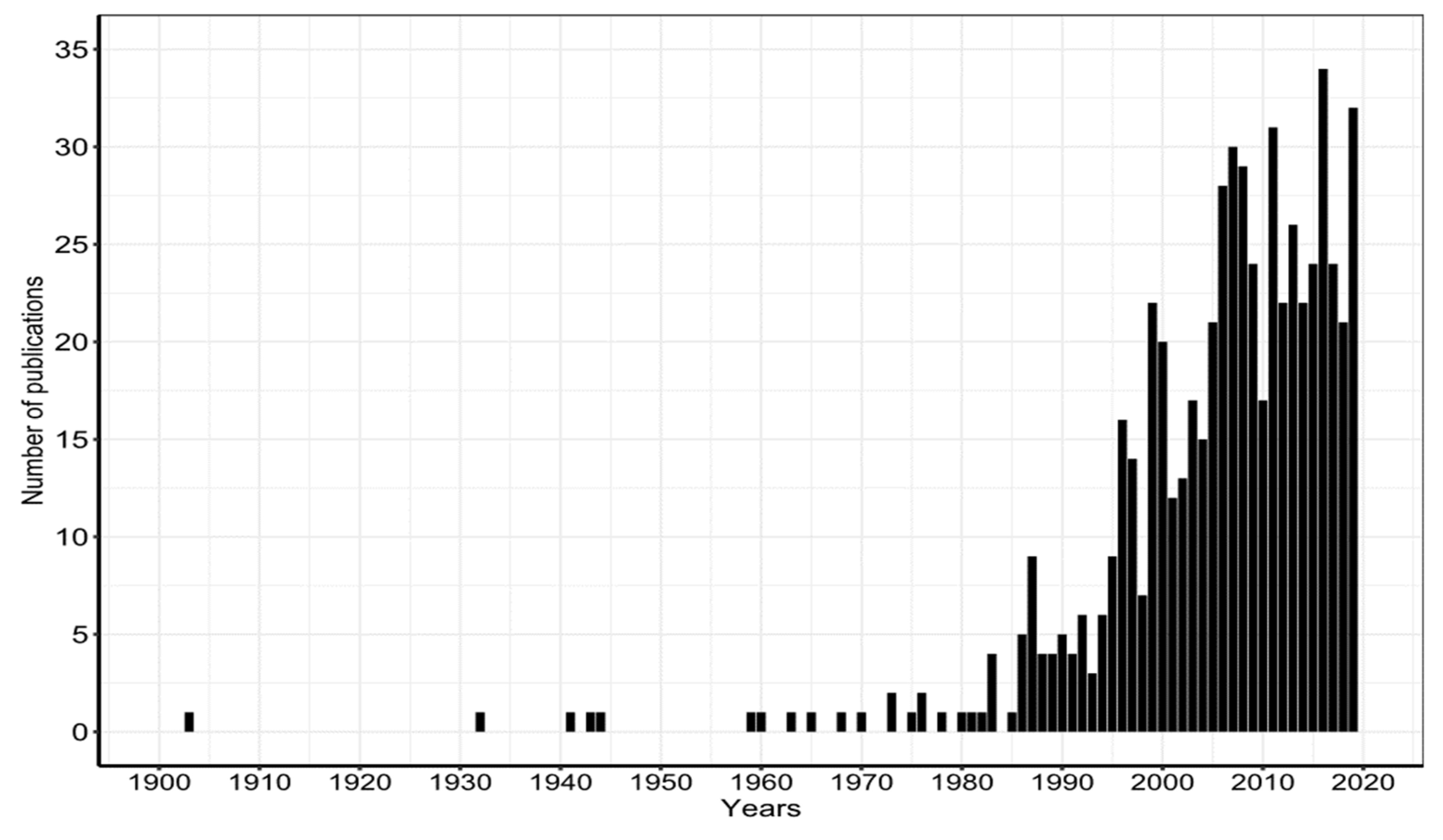
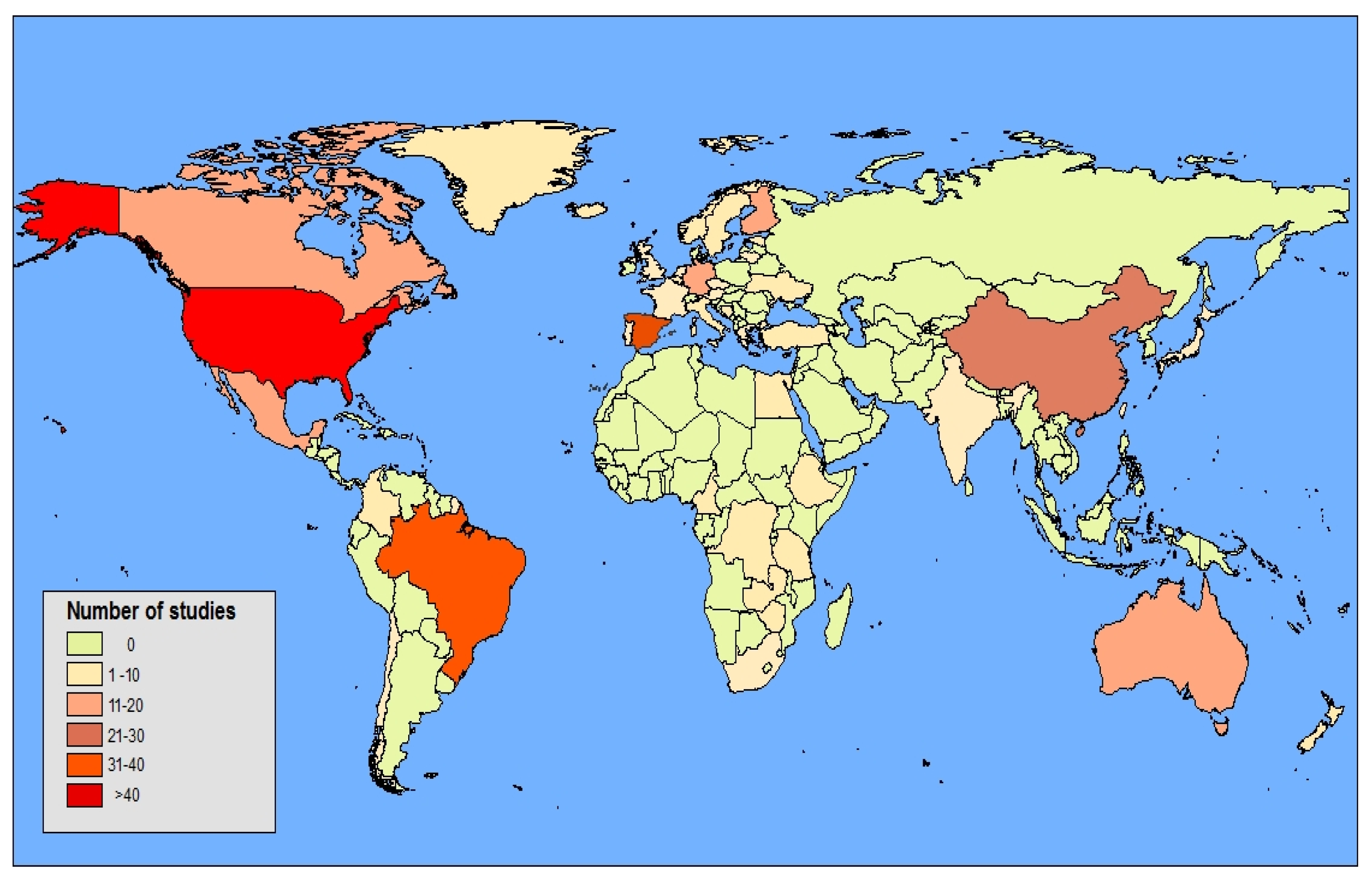
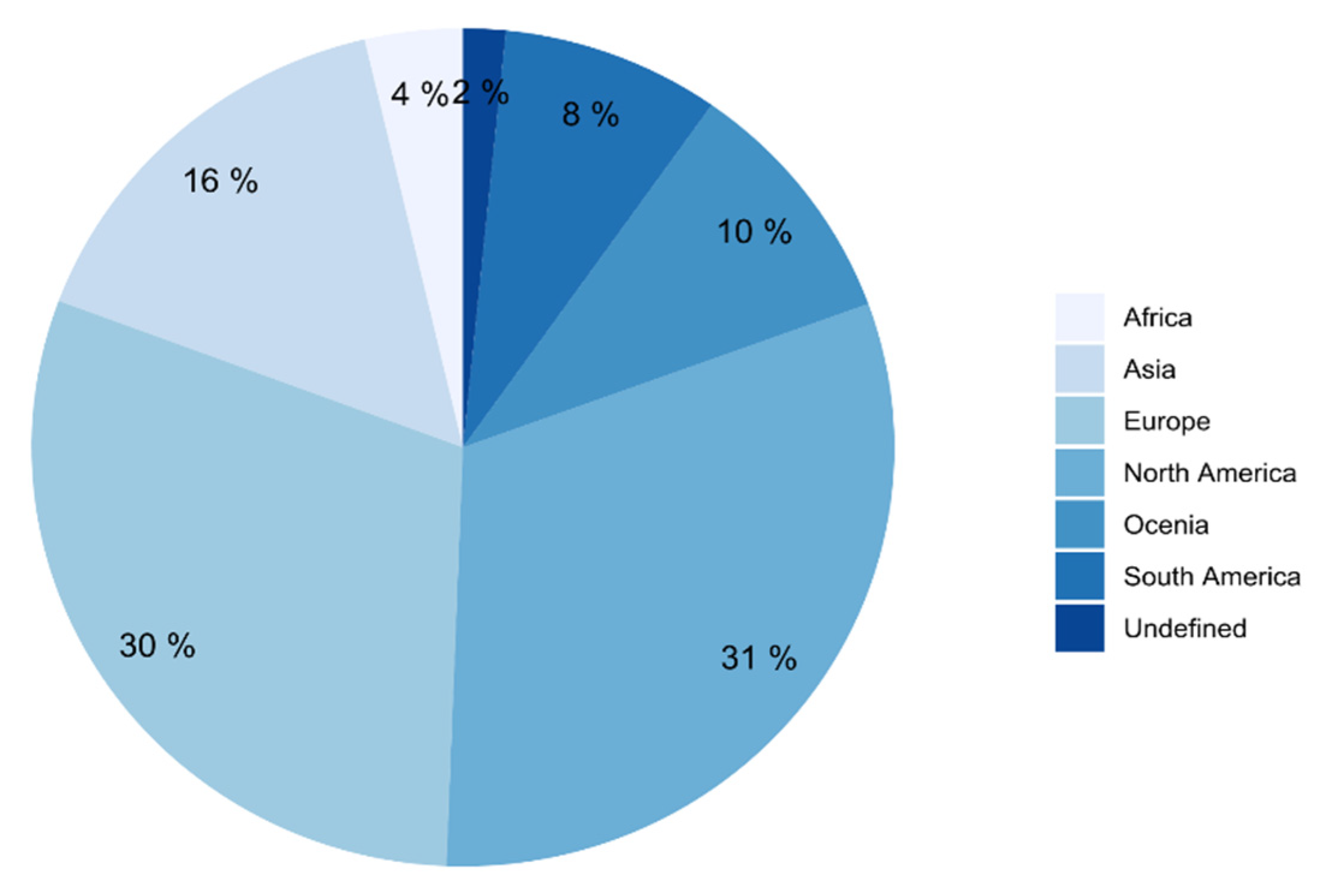
3. Frequency and Geographic Distribution of Taper Functions

Studies of tree taper extend back as far as the early 20th century, though only 25 studies were published between 1903 and 1985. The proliferation of research into the area began in 1985 and the development and use of taper functions increased markedly since the year 2000 (see Figure 2), during which time no fewer than ten studies per year have been published.

The literature shows that most of the studies on taper functions included in this study were conducted in Europe, North, Central, and South America. Countries such as the United States of America (USA) and Brazil have produced many studies on tree stem taper (Figure 3). Other parts of the world such as Asia and Australia had relatively fewer studies focusing on taper function, while there is a clear dearth of taper research in African countries. It is important to understand that the methods used in this literature review excluded non-English language journal articles, which undoubtedly biases the geographic context of the results. Moreover, many taper functions may have been developed, but only reported in white or grey literature, neither of which were included as part of this literature review. The reported results should be interpreted in this context.

Most of the functions developed in these studies were based on tree species such as pine (Pinus spp.), spruce (Picea spp.), and eucalypts (Eucalyptus spp.). Most of the studies reported on a single tree species, and research on multiple tree species is still limited, especially for the tropical regions. Establishing taper equations for tree species in the tropics is a complex exercise, which may explain the limited amount of research to date that has focused on this topic. Tropical forests contain species with irregular stem forms [22], for example, buttresses [23,24]. As a result, predicting the diameter at any height along the stem, and subsequently merchantable volume, is challenging [25]. Tropical forest species provide multi-dimensional, noisy, strongly non-linear data, and so conventional statistical procedures applied to taper modelling cannot be applied [26]. Another notable challenge to develop taper equations for tropical forest species is related to accessibility [27]; working with these species is time consuming and requires considerable financial resources [28]. Notwithstanding these challenges, establishing taper equations for tropical forests is a great opportunity, as these equations could help to inform forest conservation and sustainable timber production practices, as well as provide more accurate carbon balance estimates [25,29].

4. Forest Types of Studied Taper Functions

A total of 65% of studies focused on coniferous tree species, which is almost seven times higher than broadleaf species (9% of studies); 26% of studies developed taper functions for mixed conifer and broadleaf forests. Most often, taper functions were developed for species used in commercial plantations or production monoculture forestry. The genera most reported upon were Pinus spp., Picea spp., Quercus spp., and Eucalyptus spp., although the published studies covered a wide range of species and ecosystems, e.g., boreal, temperate, or Mediterranean. Studies on tropical forest species and mixed forest situations were very scarce, though there were some studies of Eucalyptus spp. and teak (Tectona grandis L.f.) [30,31] (

Table 1. Base taper function coefficients and goodness-of-fit statistics with brief descriptions.

Equation	Coefficients								Species	Stat., Unit	Value	Country
1	$\mathrm{Not}\mathrm{available}$								-	-	-	-
2	$\mathrm{a}=0.448$ * $\mathrm{b}=0.716$ * $\mathrm{b}=-0.082$ * * Form class = 75								Picea abies (L.) Karst.	-	-	USA
3	$\mathrm{a}=0.333$ * $\mathrm{b}=0.667$ * * Form class = 75								Picea abies (L.) Karst.	SEE vol. (%)	±13.74	USA
4	$\mathrm{a}=1.07923$ $\mathrm{b}=-1.1175$								Tsuga heterophylla (Raf.) Sarg.	-	-	USA
5	${\mathrm{b}}_1=9.127$, ${\mathrm{b}}_2=$ −1.976 ${\mathrm{b}}_3=$ 8.238, ${\mathrm{b}}_4=$ −4.964 ${\mathrm{b}}_5=3.773$, ${\mathrm{b}}_6=$−7.417								Alnus rubra (Bong.)	SEE, in $\frac{{\mathrm{d}}^2}{{\mathrm{D}}^2}$	0.0704	USA
6	$\mathrm{a}=1.116233$ $\mathrm{b}=1.405224$								Pinus resinosa Sol. Ex Aiton	SSE, D (cm)	446.634	USA
	$\mathrm{a}=0.941520$ $\mathrm{b}=1.505741$								Pinus taeda L.	SSE, D (cm)	526.285	USA
7	Not available								Populus tremuloides Michx.	-	-	CAN
8	${\mathrm{b}}_1=0.5144$ ${\mathrm{b}}_2=0.4433$								Populus tremuloides Michx. (Coastal)	SEE, D (inch)	0.59	CAN
	${\mathrm{b}}_1=0.3087$ ${\mathrm{b}}_2=0.5364$								Pseudotsuga menziesii (Mirbel) Franco (Interior)	SEE, D (inch)	1.33	CAN
9	${\mathrm{b}}_1=-3.0257$, ${\mathrm{b}}_2=1.4586$ ${\mathrm{b}}_3=-1.4464$, ${\mathrm{b}}_4=39.1081$ ${\mathrm{a}}_1=0.7431$, ${\mathrm{a}}_2=0.1125$								Pinus taeda L.	MAD, D (cm)	0.53–0.86	USA
10	${\mathrm{b}}_1=0.973539$, ${\mathrm{b}}_2=63.079675$ ${\mathrm{b}}_3=-3.408825$, $\mathrm{c}=0.004322$ ${\mathrm{a}}_1=$0.914280, ${\mathrm{a}}_2=0.275954$								Pinus resinosa Sol. Ex Aiton	SSE, D (inch)	268.918	USA
	${\mathrm{b}}_1=0.906743$, ${\mathrm{b}}_2=149.933632$ ${\mathrm{b}}_3=-2.663458$, $\mathrm{c}=0.003181$ ${\mathrm{a}}_1=0.923505$, ${\mathrm{a}}_2=0.234427$								Pinus taeda L.	SSE, D (inch)	294.163
11	${\mathrm{b}}_1=2.58$${\mathrm{b}}_2=-0.763$ ${\mathrm{b}}_3=0.205$${\mathrm{b}}_4=-0.244$								Pinus resinosa Sol. Ex AitonPicea mariana (Mill.) Britton	ME % Vol.	3.92	CAN
12	${\mathrm{a}}_0=0.77460$, ${\mathrm{a}}_1=1.04032$ ${\mathrm{a}}_2=0.99698$, ${\mathrm{b}}_1=0.74575$ ${\mathrm{b}}_2=-0.13018$, ${\mathrm{b}}_3=0.55882$ ${\mathrm{b}}_4=-0.32418$, ${\mathrm{b}}_5=0.19869$ $p=0.25$								Pinus contorta	SEE, D (cm)	1.39	CAN
	${\mathrm{a}}_0=1.21697$,${\mathrm{a}}_1=0.84256$ ${\mathrm{a}}_2=1.00001$, ${\mathrm{b}}_1=1.55322$ ${\mathrm{b}}_2=-0.39719$, ${\mathrm{b}}_3=2.11018$ ${\mathrm{b}}_4=-1.1416$, ${\mathrm{b}}_5=0.09420$ $p=0.30$								Thuja plicata	SEE, D (cm	6.67
13	${\mathrm{b}}_1=-0.569$${\mathrm{b}}_2=0.0741$ ${\mathrm{b}}_3=0.01924$								Quercus phellos (L.)	SEE d (cm)	1.284	USA
14	Species		Region		K1 × 102		K2		Mixed Species	Bias % vol.	−8.2	USA
	Cottonwood		C + I		0.20302		0.37223
	Douglas-Fir		C		0.167216		0.306585
	Douglas-Fir		I		0.181694		0.33313			Bias % vol.	−12.2
	Lodgepole pine		C + I		0.226124		0.41459
	Yellow cedar		C + I		0.219329		0.402132
	Yellow pine		C + I		0.208576		0.382417			Bias % vol.	−7.7
	Region: C= Coastal, I = Interior
19	${\mathrm{b}}_1=22.686$, ${\mathrm{b}}_2=$ −44.310 ${\mathrm{b}}_3=$ 26.708, ${\mathrm{b}}_4=$ −3.5452 ${\mathrm{b}}_5=1.1714$, ${\mathrm{b}}_6=$ 0.33021 ${\mathrm{b}}_7=$ 17.070								Pinus radiata D.Don	SEE, D (cm)	1.43	NZL
20/21	Not available								Pseudotsuga menziesii (Mirbel) Franco; Acer spp. (L.)	SEE D (inch)	0.72/0.49	CAN
22	${\mathrm{a}}_0=0.93242$, ${\mathrm{a}}_1=0.99682$ ${\mathrm{b}}_1=0.38479,$${\mathrm{b}}_2=0.13417$ ${\mathrm{b}}_3=0.04151$, ${\mathrm{b}}_4=-0.14300$ ${\mathrm{b}}_5=0.00015$, ${\mathrm{b}}_6=0.44204$ ${\mathrm{b}}_7=-0.44441$								Pinus contorta	SEE, D (cm)	0.6468	CAN
23	${\mathrm{b}}_1=2.1288$, ${\mathrm{b}}_2=-0.63157$ ${\mathrm{b}}_3=-1.6082$, ${\mathrm{b}}_4=2.4886$ ${\mathrm{b}}_5=-2.4147$, ${\mathrm{b}}_6=2.3619$ ${\mathrm{b}}_7=-1.7539$, ${\mathrm{b}}_8=1.0817$								Pinus spp.	SEE, D (%)	3.63	CAN
24	u	Coefficient							Pinus sylvestris (L.)	RMSE, vol. (%)	3.5	FIN
		a0		a1		a2		a3
	1	0.784		0.958		0.034		−0.118
	2	0.793		0.897		0.043		−0.123
	3	0.746		0.853		0.052		−0.124
	4	0.558		0.933		0.033		−0.111
	5	0.521		0.903		0.038		−0.101
	6	0.483		0.862		0.046		−0.09
	7	318		0.866		0.042		−0.057
	8	0.065		0.939		0.019		−0.011
	9	−0.313		1.054		−0.018		0.056
	10	−0.644		1.12		−0.044		0.113
	11	−1.141		1.194		−0.073		0.169
	12	−1.798		1.23		−0.093		0.206
	13	−0.63		1.276		−0.108		0.23
	14	−2.168		1.396		−0.162		0.524

Note: Eq. = Equation number following different types of taper functions; different numbers and forms of a, b, and K are coefficients; Stat., Units = goodness-of-fit statistics and their units; abbreviations of countries follow ISO 3166; SEE = sum of estimated errors; SSE = sum of squared error; MAE = mean absolute error; MAD = mean absolute deviation; ME = mean error; RMSE = root mean squared error; D = diameter (cm or inch or %); Vol. = volume; abbreviations of countries follow ISO 3166.

and Table 2).

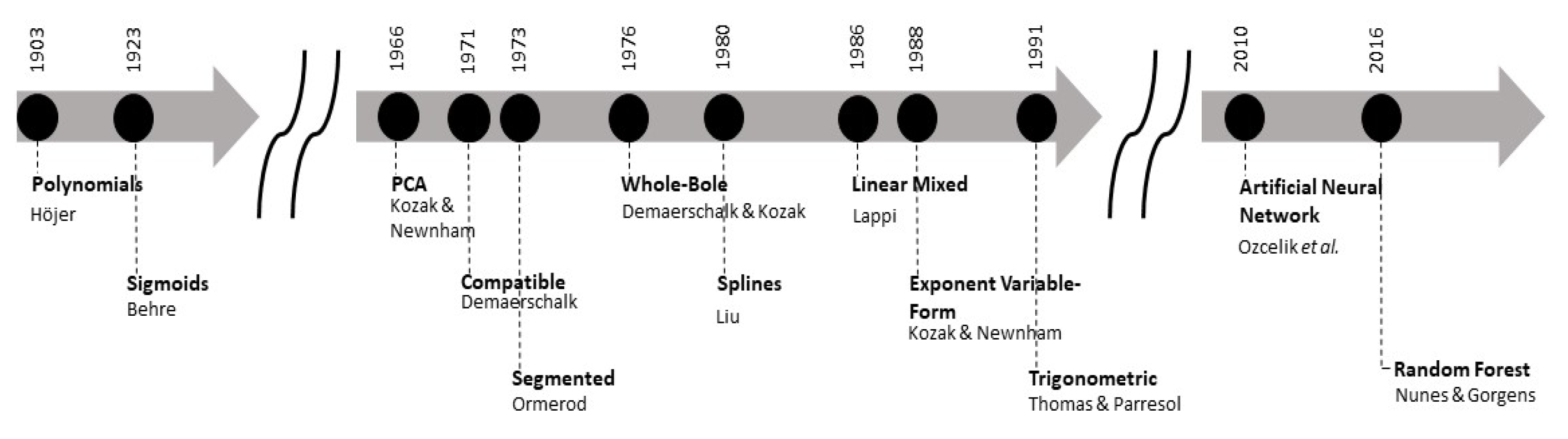
5. A Brief History of Taper Functions

Höjer [32] developed the first taper function from measurements of Norway spruce (Picea abies (L.) H. Karst) in Sweden. This function gives the diameter at any point on the stem as a percentage of diameter at breast height. Jonson [33] showed that Höjer’s [32] formula conformed closely to the measured taper. This function was further calibrated and improved by introducing stand- and species-specific information. Later, Behre [17] proposed a sigmoidal way to model stem curve from western yellow pine measurements. Multivariate methods for construction of an integrated system of models of tree taper curves were introduced in the 1960s [34,35], one of which was principal component analysis (PCA) [36]. This integrated system was expected to overcome the limitations of previously used methods. Grosenbaugh [37] also observed that, although the polynomial method was less efficient, it was a mathematically rational analysis.

In the early 1970s, Demaerschalk [21] introduced the theory of compatible taper and volume equation systems to make these functions more rational and useful. Demaerschalk [21,38] developed ways to ensure that compatible taper equations, when integrated, produce an identical estimate of total volume to that given by tree-level volume equations. Since then, the compatibility concept has been explored and expanded, and several approaches for developing compatible systems of taper and volume have been proposed [39]. However, most equations developed for volume and upper bole diameter estimates are of an empiric, rather than geometric origin. As such, these equations are of limited use, and they need a general, species-specific, stem profile model that can be integrated to give a desirable volume equation [7]. For that reason, Ormerod [20] considered a simple and flexible whole bole geometric model. Later, the common and convenient assumption of tree bole segmentation with various geometric solids was applied. In this case, the whole tree bole was considered and modelled as a series of different frustums, and finally combined as one single model [40,41].

In general, all these polynomials and their variable exponent forms of taper functions are parametric. Despite their wide use and varying model forms, comparisons of taper equation performance in predicting both stem form and volume for a given species are less common [12]. Moreover, Assis et al. [15] pointed out the challenge of using a single taper approach to describe different species and a wide range of tree size classes. Bi [42] suggested a trigonometric method but indicated a problem with the number of parameters of limited biological interpretation in most taper equations. Thus, a lack of flexibility could easily result in highly biased estimates even within a species [6]. Therefore, the most accurate taper functions may be species-, tree size class-, and region-specific. This specificity highlights the need for the development of a generalised and flexible approach.

Consequently, semi-parametric and nonparametric methods aimed to fill the gap of developing generalised and flexible functions. These methods included a semi-parametric smoothing spline [43], B-splines [44], generalised additive models [45], and neural networks [46]. Robinson et al. [45] reported that semi-parametric methods performed like a more traditional parametric approach for predicting whole-stem volume, merchantable volume, number of logs, small-end diameter of the first log, and volume of the first log. On the other hand, Özçelik et al. [46] suggested that a nonparametric neural network was superior to the parametric approach. Penalised splines are robust and flexible for stem taper and volume [47]. This is an evolution of the splines, which are well known for avoiding under- or over-fitting and for avoiding poorly behaved estimation in the tails. However, inference might be difficult as the smoothing function is based on a penalisation criterion [47]. Pedan [48] proposed mixed-effects modelling to overcome the difficulties of penalised spline regression. The key milestones are recorded in Figure 4.

6. Types of Taper Function

Since their inception, several types of taper function have been developed. Based on the development approach, they are mainly classified as parametric or non-parametric approaches.

6.1. Parametric Taper Equations

A wide variety of taper functions have been fitted through different regression approaches. These include purely parametric statistical procedures such as ordinary least squares (OLS) (e.g., [49]), nonlinear least squares (NLS) (e.g., [50]), or semi-parametric statistical procedures such as spline [43], and generalised additive models (GAM) [45]. All these taper functions range from simple to complex. Specifically, they include polynomial, sigmoid, segmented polynomial, compatible, and whole-bole-system taper functions. The characteristics and applications of these different taper functions are presented in Section 6.1.1 and Section 6.1.2.

6.1.1. Static Taper Equations

Static taper functions assume that the changes in the diameter at breast height (D) could reflect changes in upper stem diameters without the inclusion of time or age in the model. This taper equation usually predicts the ratio of diameter or radius at a specific distance from the tip to calculate the volume of the sections of a tree [3]. The general form of this type of equation is presented in Equation (1):

$$\mathrm{y}=\mathrm{k}\sqrt{{\mathrm{x}}^{\mathrm{r}}}$$

(1)

where y is the radius or diameter at a specific distance x from the tip, k is a constant, and r is a form exponent that changes with the geometric solids that reflect different parts of the stem.

Polynomial Form Models

Behre [17] reported on the development of the first taper Equation (2) for P. abies:

$$\frac{\mathrm{d}}{\mathrm{D}}=\mathrm{Clog}\left(\frac{\mathrm{c}-\mathrm{l}}{\mathrm{c}}\right)$$

(2)

where d is the diameter inside the bark at distance l from the tip, D is the diameter at breast height, and C and c are constants. A new taper equation was then developed with a hyperbolic form (Equation (3)):

$$\frac{\mathrm{d}}{\mathrm{D}}=\frac{\left(\frac{\left(\mathrm{H}-\mathrm{h}\right)}{\mathrm{h}}\right)}{{\mathrm{b}}_0+{\mathrm{b}}_1\left(\frac{\left(\mathrm{H}-\mathrm{h}\right)}{\mathrm{h}}\right)}$$

(3)

where d is the diameter inside the bark at height h, D is the diameter at breast height, H is the total height, and b₀ and b₁ are parameters.

Equation (3) is a more useful form than Equation (2). The parameters of Equation (3) can be linearly extended by augmenting them with biologically relevant variables, and the equation can be inverted to predict h. However, in consideration of closed form integration, Equation (2) is superior to Equation (3).

Kozak and Smith [36] developed a simple equation that was a paraboloid and this equation resulted in a low standard error compared with the previous version (Equation (4)):

$$\mathrm{d}=\mathrm{D}\sqrt{\mathrm{a}+\mathrm{b}\left(\frac{\mathrm{h}}{\mathrm{H}-4.5}\right)}$$

(4)

where d is the diameter inside the bark at height h, D is the diameter at breast height, H is the total height, and a and b are parameters.

Bruce et al. [7] developed a polynomial taper equation (Equation (5)) for Alnus rubra (Bong.), which includes a series of exponents for representing different parts of the stem. This equation has been used for a number of hardwoods and softwoods throughout the world.

$$\begin{gathered} \frac{{\mathrm{d}}^2}{{\mathrm{D}}^2}={\mathrm{b}}_1{\mathrm{x}}^{\frac{3}{2}}+{\mathrm{b}}_2\left({\mathrm{x}}^{\frac{3}{2}}-{\mathrm{x}}^3\right)\mathrm{D}+{\mathrm{b}}_3\left({\mathrm{x}}^{\frac{3}{2}}-{\mathrm{x}}^3\right)\mathrm{H}+{\mathrm{b}}_4\left({\mathrm{x}}^{\frac{3}{2}}-{\mathrm{x}}^{32}\right)\mathrm{H}\times \mathrm{D} \\ +{\mathrm{b}}_5\left({\mathrm{x}}^{\frac{3}{2}}-{\mathrm{x}}^{32}\right)\sqrt{\mathrm{H}}+{\mathrm{b}}_6\left({\mathrm{x}}^{\frac{3}{2}}-{\mathrm{x}}^{40}\right){\mathrm{H}}^2 \end{gathered}$$

(5)

where d is the diameter inside the bark at height h, D is the diameter at breast height, H is the total height $\mathrm{x}=\left(\frac{\mathrm{H}-\mathrm{h}}{\mathrm{H}-4.5}\right)$, and ${\mathrm{b}}_1$ to ${\mathrm{b}}_6$ are parameters.

Sigmoid Taper Equations

Ormerod [20] described the form of tree stems with a simple sigmoid equation. Other transformations of Equation (6) have been reported in Byrne and Reed [8]:

$$\mathrm{d}={\mathrm{b}}_1\mathrm{D}{\left(\frac{\mathrm{H}-\mathrm{h}}{\mathrm{H}-\mathrm{BH}}\right)}^{{\mathrm{b}}_2}$$

(6)

where d is the diameter inside the bark at height h, D is the diameter at breast height, H is the total height, BH is the breast height, and b₁ and b₂ are parameters.

Forslund [51] used a simple sigmoidal equation to define the taper of aspen (Populus tremuloides Michx). The model has the form presented in Equation (7):

$$\mathrm{Y}={\left(1-{\mathrm{X}}^{\mathrm{a}}\right)}^{\left(\frac{1}{\mathrm{b}}\right)}$$

(7)

where Y = d/D, d is the diameter at the upper position, D is the basal diameter, X = h/H, h is the height to the measurement position from the base of the stem, H is the total height, and a and b are parameters.

Segmented Polynomial Taper Equations

Ormerod [20] also developed a geometrically segmented taper equation (Equation (8)) using inflection points for different sections of the stem. The data for fitting the equation came from smoothed taper curves that were developed in British Columbia, Canada.

$$\mathrm{d}=\left({\mathrm{d}}_{\mathrm{j}}-{\mathrm{C}}_{\mathrm{i}}\right){\left(\frac{{\mathrm{H}}_{\mathrm{i}}-\mathrm{h}}{{\mathrm{H}}_{\mathrm{i}}-{\mathrm{h}}_{\mathrm{j}}}\right)}^{{\mathrm{p}}_{\mathrm{i}}}+{\mathrm{C}}_{\mathrm{i}}$$

(8)

where d is the estimated diameter at the upper position, h is the height to the estimated diameter position from the base of the section, H_i is the height to the top of the section, h_j is the height to the measured diameter d_j, p_i is the fitted exponent for the section, and C_i is the intercept of sectional diameter.

On the other hand, Max and Burkhart [41] developed a statistical segmented taper model for loblolly pine (Pinus taeda L.) in the USA. In this model, the sum of squared error for the sub-models was minimised by restricting the continuous and smooth functions at the join points. The function (Equation (9)) has been used extensively for conifers and broadleaved trees in many parts of the world [41].

$$\mathrm{d}=\sqrt{{\mathrm{D}}^2\left[{\mathrm{b}}_1\left(\frac{\mathrm{h}}{\mathrm{H}}-1\right)+{\mathrm{b}}_2\left(\frac{{\mathrm{h}}^2}{{\mathrm{H}}^2}-1\right)+{\mathrm{b}}_3{\left({\mathrm{a}}_1-\frac{\mathrm{h}}{\mathrm{H}}\right)}^2{\mathrm{I}}_1+{\mathrm{b}}_4{\left({\mathrm{a}}_2-\frac{\mathrm{h}}{\mathrm{H}}\right)}^2{\mathrm{I}}_2\right]}$$

(9)

where d, D, H, and h have been defined before; a₁ and a₂ are join points; and I₁ and I₂ have the values of 1 or 0 (dummy variables).

Variable Exponent Form Models

A new type of taper equation called a variable exponent taper equation (Equation (10)) was introduced by Newnham [52,53]. These are continuous functions where the exponent varies from the ground to the tip in order to compensate for different shapes.

$$\mathrm{Y}={\mathrm{x}}^{1/\mathrm{k}}$$

(10)

where $\mathrm{Y}=\left(\frac{\mathrm{d}}{\mathrm{D}}\right)$; $\mathrm{x}=\left(\frac{\mathrm{H}-\mathrm{h}}{\mathrm{H}-\mathrm{BH}}\right)$; $\mathrm{k}={\mathrm{b}}_0+{\mathrm{b}}_1\left(\frac{\mathrm{D}}{\mathrm{H}}\right)+{\mathrm{b}}_2\mathrm{x}{\left(\frac{\mathrm{D}}{\mathrm{H}}\right)}^2+{\mathrm{b}}_3{\left(\frac{1}{\mathrm{H}}\right)}^{{\mathrm{b}}_4}$. In this equation, d is the diameter inside the bark at height h and k depends on the diameter at breast height (D), total height (H), and breast height (BH).

Kozak [18], based on previous work of Newnham [52], presented a variable exponent equation (Equation (11)):

$$\mathrm{d}={\mathrm{a}}_0{\mathrm{D}}^{{\mathrm{a}}_1}{\mathrm{a}}_2{}^{\mathrm{D}}{\left(\frac{1-\sqrt{\mathrm{z}}}{1-\sqrt{\mathrm{p}}}\right)}^{{\mathrm{b}}_1{\mathrm{z}}^2+{\mathrm{b}}_2\ln \left(\mathrm{z}+0.001\right)+{\mathrm{b}}_3\sqrt{\mathrm{z}}+{\mathrm{b}}_4{\mathrm{e}}^{\left(\mathrm{z}\right)}+{\mathrm{b}}_5\left(\raisebox{1ex}{$\mathrm{D}$}\!\left/ \!\raisebox{-1ex}{$\mathrm{H}$}\right.\right)}$$

(11)

where d is the diameter inside the bark at height h; D is the diameter at breast height; and Z is h/H, with h and H described previously, p = HI/H, where HI is the inflection point that can be fitted depending on the species, and a₀ and a₁ as well as b₁ to b₅ are parameters.

Trigonometric Models

Thomas and Parresol [54] developed a trigonometric taper equation (Equation (12)) that includes trigonometric functions to describe stem form:

$$\mathrm{d}=\sqrt{{\mathrm{D}}^2\left[{\mathrm{b}}_1\left(\mathrm{z}-1\right)+{\mathrm{b}}_2\sin \left(\mathrm{c}\mathsf{\pi }\mathrm{z}\right)+\frac{{\mathrm{b}}_3}{-\tan \left(\mathsf{\pi }\mathrm{z}∕2\right)}\right]}$$

(12)

where z is the relative height h/H and π is Pi, the mathematical constant, and b₁, b_s, and c are parameters. The variables d, D, h, and H have been described previously.

6.1.2. Complex Taper Functions

Compatible Taper Models

The compatible taper equation (Equation (13)) was developed by Demaerschalk [21] for 16 species in the USA.

$$\frac{{\mathrm{d}}^2}{{\mathrm{D}}^2}=\mathrm{a}+\mathrm{b}\frac{\mathrm{h}}{\mathrm{H}}+\mathrm{c}\frac{{\mathrm{h}}^2}{{\mathrm{H}}^2}$$

(13)

After integrating Equation (13), volume can be obtained by the following:

$$\mathrm{V}={\mathrm{K}}_1{\mathrm{D}}^2\mathrm{H}$$

(14)

and the ratios of volume to basal area can be derived when the constant of integration is set to 0:

$$\frac{\mathrm{V}}{\mathrm{B}}={\mathrm{K}}_2\mathrm{H}$$

(15)

by solving for K₁ and K₂. The formulas for K₁ and K₂ are presented in Equations (16) and (17).

$${\mathrm{K}}_1=0.00545415\left(\mathrm{a}+\frac{\mathrm{b}}{2}+\frac{\mathrm{c}}{3}\right)$$

(16)

$${\mathrm{K}}_2=\left(\mathrm{a}+\frac{\mathrm{b}}{2}+\frac{\mathrm{c}}{3}\right)$$

(17)

where D, V, h, and H have been described previously; and a, b, and c are regression coefficients from Equation (13). d is the diameter inside the bark at the point l that is the distance from the tip; k = π/40,000 numeric units or English units in the case of Equation (16); and b₂ to b_n are parameters and n is the number of the parameter.

Whole-Bole Systems Models

Demaerschalk and Kozak [55] presented a system that consists of two functions that are linked at an inflection point of the stem. These functions are used to predict diameter inside the bark for the top of the tree (Equation (18)), and the calibrated diameter at the bottom of the tree is provided in Equation (19).

$$\mathrm{d}=\left[{\left(\frac{\frac{\mathrm{h}}{\mathrm{H}}}{\mathrm{RH}}\right)}^{{\mathrm{b}}_1}{\mathrm{b}}_2{}^{\left(1-\frac{\frac{\mathrm{h}}{\mathrm{H}}}{\mathrm{RH}}\right)}\right]\mathrm{DI}$$

(18)

$$\mathrm{d}=\left[{\mathrm{b}}_3-\left({\mathrm{b}}_3-1\right){\left(\frac{1-\frac{\mathrm{h}}{\mathrm{H}}}{\mathrm{RHI}}\right)}^{{\mathrm{b}}_4}\right]\mathrm{DI}$$

(19)

where d is the diameter inside bark at point h, DI is the diameter inside bark at the inflection point, RH is the distance of inflection point from the tip, RHI is the distance of the inflection point from the ground level, h and H have been described previously, b₁ and b₂ are regression parameters, and b₃ and b₄ are coefficient in the conditioned tree bottom model. The system of equation [55] is illustrated in the Supplementary Material (Figure S1). It is important to note that no coefficients were available for the system in the original publications.

Dynamic Taper Models

Muhairwe [56] developed a dynamic taper equation to include time in the diameter estimations (Equation (20)).

$${\hat{\mathrm{d}}}_{\mathrm{ijt}}={\mathrm{a}}_0{\hat{\mathrm{D}}}_{\mathrm{it}}{}^{{\mathrm{a}}_1}{\left[1-\sqrt{{\hat{\mathrm{Z}}}_{\mathrm{ijt}}}\right]}^{{\mathrm{b}}_1{\hat{\mathrm{Z}}}_{\mathrm{ijt}}{}^2+{\mathrm{b}}_2\sqrt{{\hat{\mathrm{Z}}}_{\mathrm{ijt}}}+{\mathrm{b}}_3\frac{{\hat{\mathrm{D}}}_{\mathrm{it}}}{{\hat{\mathrm{H}}}_{\mathrm{it}}}+{\mathrm{b}}_4\frac{1}{{\mathrm{Age}}_{\mathrm{it}}}+{\mathrm{b}}_5{\widehat{\mathrm{QD}}}_{50\mathrm{K}}{}^2+{\mathrm{b}}_6\frac{1}{{\hat{\mathrm{H}}}_{\mathrm{it}}}+{\mathrm{b}}_7\frac{1}{{\mathrm{h}}_{\mathrm{ijt}}+0.001}}$$

(20)

where ${\hat{\mathrm{d}}}_{\mathrm{ijt}}$ is the estimated diameter at breast height for the tree i, section j, and time t; ${\hat{\mathrm{D}}}_{\mathrm{it}}$ is the predicted diameter at breast height for the tree i at time t; ${\hat{\mathrm{H}}}_{\mathrm{it}}$ is the predicted tree height for the tree i at time t; ${\mathrm{h}}_{\mathrm{ijt}}$ is the height for the tree i, section j, and time t; ${\mathrm{Age}}_{\mathrm{it}}$ is the breast height age of the tree i at time t; ${\hat{\mathrm{Z}}}_{\mathrm{ijt}}$ is the predicted relative height; ${\widehat{\mathrm{QD}}}_{50\mathrm{k}}$ is the quadratic mean diameter at age 50 years for plot k; and a₀ and a₁ as well as b₁ to b₇ are parameters.

Other Complex Taper Models

Laasasenaho [57] developed a taper function (Equation (21)) that is a simultaneous model containing all the diameters measured at different relative heights in the stem.

$$\frac{{\mathrm{d}}_{\mathrm{l}}}{{\mathrm{d}}_{0.2\mathrm{h}}}={\mathrm{c}}_1{\mathrm{x}}^1+{\mathrm{c}}_2{\mathrm{x}}^2+{\mathrm{c}}_3{\mathrm{x}}^3+{\mathrm{c}}_4{\mathrm{x}}^5+{\mathrm{c}}_5{\mathrm{x}}^8+{\mathrm{c}}_6{\mathrm{x}}^{13}+{\mathrm{c}}_7{\mathrm{x}}^{21}+{\mathrm{c}}_8{\mathrm{x}}^{34}$$

(21)

where d_l is the diameter inside bark at distance l from the ground level, d_0.2h is the diameter at 20% of the tree height, $\mathrm{x}=\left(1-\left(\frac{\mathrm{l}}{\mathrm{h}}\right)\right)$ or the relative distance from the top, and c₁ to c₈ are the fitted parameters.

Lappi [19] developed a linear-mixed model for predicting stem forms that are represented for diameter and height using polar coordinates (Equation (22)) (see Figure S2 in the Supplementary Materials for an illustrative figure).

$${\mathrm{d}}_{\mathrm{ki}}\left(\mathrm{u}\right)={\mathrm{a}}_0\left(\mathrm{u}\right)+{\mathrm{a}}_1\left(\mathrm{u}\right){\mathrm{s}}_{\mathrm{ki}}+{\mathrm{a}}_2\left(\mathrm{u}\right){\mathrm{s}}_{\mathrm{ki}}{}^2-{\mathrm{a}}_3\left(\mathrm{u}\right)\left({\mathrm{s}}_{\mathrm{ki}}-\overline{{\mathrm{s}}_{\mathrm{k}.}}\right)+{\mathrm{v}}_{\mathrm{k}}\left(\mathrm{u}\right)+{\mathrm{e}}_{\mathrm{ki}}\left(\mathrm{u}\right)$$

(22)

where ${\mathrm{a}}_{\mathrm{i}}\left(\mathrm{u}\right)={\mathrm{a}}_{\mathrm{o}}\left(\mathrm{u}\right)+-\mp {\mathrm{a}}_{\mathrm{i}}\left(\mathrm{u}\right)$; ${\mathrm{d}}_{\mathrm{ki}}\left(\mathrm{u}\right)$ is the logarithmic diameter i at angle u for the stand k; u is the angle measured from the ground level; ${\mathrm{s}}_{\mathrm{ki}}$ is the logarithmic size of the tree; $\overline{{\mathrm{s}}_{\mathrm{k}}}$ is the average size for the stand k; ${\mathrm{v}}_{\mathrm{k}}$ and ${\mathrm{e}}_{\mathrm{ki}}$ are the random stand effect and random tree effect, respectively; and a₀ to a₃ are fixed parameters.

Contemporary Taper Models

Apart from all the mathematical parametric and semi-parametric methods, the use of artificial intelligence (AI) tools as a non-parametric method was introduced in taper modelling by Özçelik et al. [46]. So far, this has been done by using a regression tree algorithm named random forest (RF) and artificial neural network (ANN) [25,46]. In the most complex cases, ANN outperformed RF methods in terms of precise prediction; however, the RF algorithm proved to be the most generalisable [25]. Both of these methods work through a trial-and-error method, testing a range of possible values and then verifying through fitting statistics [58].

6.2. Non-Parameric Taper Equations

In the most recent decade, non-parametric methods have been gaining popularity in modelling tree taper. These methods are based on ensemble methods such as machine learning or deep learning (DL) algorithms, which create multiple models and combine them to produce results. So far, different computational algorithms for artificial neural networks (ANNs) [46] and random forest (RF) regression trees [25] have been explored. For example, three different multilayer perceptron algorithms were tested for ANN, namely, backward, forward, and cascade correlation propagated perceptron neural networks [46]. Nonparametric approaches have generally been reported to have superior predictive quality over traditional parametric approaches [25,59]. However, McTague and Weiskittel [16] reported that nonparametric approaches are highly data sensitive, tend to overpredict, and hence are not capable of explaining the underlying biological processes.

7. Parameters and Accuracy of Taper Functions

Researchers often compare the most commonly used functions. In most cases, parameters for similar species from different regions are used as a starting point for testing existing functions. In addition, the collection of reliable parameter values is important; however, this is usually expensive and time consuming. For example, Breuer et al. [60] noticed similar phenomena for plant ecophysiological models in temperate climatic zones and reported that (i) a lot of these investigations on taper functions are relatively old and are not available through current databases, and (ii) the breadth of current scientific databases is quite extensive. As a result, the functions and parameters used in most cases are not particularly suitable. In other cases, looking at a small range of parameters results in high spatial and temporal variability [60]. A current content database search can change this scenario, especially as studies on taper functions have increased steadily after 1980 (Figure 1). However, there is a lack of accessible compiled information, which is inevitably important.

Realizing that there is no comprehensive overview of parameters for parametric taper functions, this study included a comprehensive literature review of taper functions and their parameters. Various studies reported and used different measures with different measurement units to quantify the accuracy or goodness-of-fit (Table 1). In the case of complex taper equations, the number of parameters increased and often included sub-parameters. The taper function studies with reported parameters and accuracy were continentally dominated by Europe and the Americas (Figure 5). Most of the studies compiled here reported on either parameters and goodness-of-fit statistics or both; 78% of studies showed parameters used in taper functions, while 84% showed goodness-of-fit statistics for taper functions. In contrast, some studies failed to report estimated parameters, goodness-of-fit statistics, or in some cases both; for example, Byrne and Reed [8] and Nicoletti et al. [61].

Table 2. Species-specific taper functions.

Types of Taper Functions	Species	Country	Reference
Non-parametric (ML)	Acacia mearnsii (De Wild.)	BRA	Schikowski, et al. [62]
Static, segmented polynomial, and variable-exponent	Abies nordmanniana (subsp. bornmulleriana Mattf.)	TUR	Sakici, et al. [63]
Variable-exponent equation	Alnus rubra (Bong.)	USA, CAN	Hibbs, et al. [64]
Static polynomial equation	Araucaria cunninghamii (Ait. ex D. Don)	AUS	Allen, et al. [65]
Segmented polynomial	Betula platyplhylla (Sukaczev)	CHN	Shahzad, et al. [66]
Single and segmented polynomial	Betula alnoides	CHN	Tang, et al. [67]
Segmented polynomial	Calocedrus formosana	TWN	Wang, et al. [68]
Non-parametric (AI)	Cryptomeria japónica	BRA	Sanquetta, et al. [69]
Sigmoid equation	Cryptomeria japónica. D. Don.	JPN	Hada [70]
Segmented polynomial	Eucalyptus grandis × E. urophylla (Hybrid) E. grandis × E. camaldulensis (Hybrid)	ZAF	Morley and Little [71]
Static polynomial	Eucalyptus grandis × Eucalyptus urophylla (Hybrid)	BRA	Da Silva, et al. [72]
Compatible taper equation	Eucalyptus pilularis; E. obliqua; E. andrewsii; E.saligna; Corymbia maculata	AUS	Muhairwe [30]
Static polynomial	Eucalyptus cloeziana (f. Muell.)	ZMB	Eerikäinen, et al. [73]
Variable-exponent equation	Eucalyptus saligna	CMR	Fonweban [74]
Non-parametric (ANN)	Fagus orientalis Abies nordmanniana	TUR	Sakici and Ozdemir [75]
Segmented polynomial	Larix gmelinii (Rupr.)	CHN	Liu, et al. [76]
Dynamic taper equation	Nothofagus spp.	CHL	Valenzuela, et al. [77]
Segmented polynomial	Picea abies (L.) H. Karst.	CZE	Adamec, et al. [78]
Sigmoid (Spline) taper equation	Picea abies (L. Karst.)	CZE	Kuželka and Marušák [79]
Variable-exponent	Picea sitchensis (Bong. Carr.) Pinus sylvestris (L.)	GBR	Fonweban, et al. [10]
Variable-exponent equation	Picea glauca (Moench. Voss)	CAN	Huang, et al. [80]
Polynomial	Pinus nigra (J.F. Arnold)	ITA	Marchi, et al. [81]
Segmented polynomial	Pinus elliottii × P. caribaea var. hondurensis (Pexc)	ZAF	Algera, et al. [82]
Compatible taper equation	Pinus cooperi Pinus durangensis	MEX	Corral-Rivas, et al. [83]
Mixed segmented compatible	Pinus brutia (Ten.) Pinus nigra (Arnold.)	TUR	Özçelik, et al. [84]
Segmented polynomial	Pinus sylvestris (L.); Pinus pinaster (Ait.); Quercus pyrenaica (Willd.); Populus x euramericana (Dode); Pinus pinea (L.); Juniperus thurifera (L.); Pinus nigra (Arnold.); Fagus sylvatica (L.)	ESP	Rodríguez, et al. [85]
Semi-parametric	Pinus spp. and Quercus spp.	MEX	Návar [86]
Variable-exponent equation	Pinus banksiana (Lamb.) Picea mariana (Mill. BSP)	CAN	Subedi, et al. [87]
Segmented polynomial	Pinus contorta Larix sibirica	ISL	Heidarsson and Pukkala [88]
Segmented polynomial	Pinus sylvestris (L.)	TUR	Özçelik [89]
Compatible taper equation	Pinus taeda (L.)	USA	Coble and Hilpp [90]
Variable-exponent equation	Pinus pinaster (Ait.)	ESP	Rojo, et al. [91]
Variable-exponent equation	Pinus taeda (L.)	USA	Bullock and Burkhart [92]
Static polynomial equation	Pinus kesiya, Pinus oocarpa, Pinus merkusii, Pinus michoacana, Eucalyptus grandis, Eucalyptus doeziana	ZMB	Heinonen, et al. [93]
Segmented polynomial	Populus hybrids (P. trichocarpa/P. deltoids)	FRA	Benbrahim and Gavaland [94]
Segmented polynomial	Pseudotsuga menziesii	ESP	López-Sánchez, et al. [95]
Compatible taper equation	Quercus variabilis	CHN	Zheng, et al. [96]
Dynamic taper equation	Quercus robur (L.)	ESP	Gómez-García, et al. [97]
Segmented polynomial	Quercus fagaceae	MEX	Pompa-García, et al. [98]
Compatible taper equation	Quercus robur L. Q petraea (Matt) Liebl	DNK	Tarp-Johansen, et al. [99]
Compatible taper equation	Quercus robur (L.)	ZAF	Trincado, et al. [100]
Compatible taper equations	Salix schwerinii (E. L. Wolf)	FIN	Salam, et al. [101]
Segmented polynomial	Taiwania cryptomerioides	TWN	Wang, et al. [102]
Mixed polynomial	Tectona grandis (L.f.)	BRA	Lanssanova, et al. [103]
Non-parametric (ANN)	Tectona grandis (Linn.)	BRA	Leite, da Silva, Binoti, Fardin and Takizawa [31]
Spline regression	Not defined	DEU	Kublin, et al. [104]

Note: Abbreviations of countries follow ISO 3166. Parameters of these studies are provided in the Supplementary Information (Table S1).

Table 2. Species-specific taper functions.

Types of Taper Functions	Species	Country	Reference
Non-parametric (ML)	Acacia mearnsii (De Wild.)	BRA	Schikowski, et al. [62]
Static, segmented polynomial, and variable-exponent	Abies nordmanniana (subsp. bornmulleriana Mattf.)	TUR	Sakici, et al. [63]
Variable-exponent equation	Alnus rubra (Bong.)	USA, CAN	Hibbs, et al. [64]
Static polynomial equation	Araucaria cunninghamii (Ait. ex D. Don)	AUS	Allen, et al. [65]
Segmented polynomial	Betula platyplhylla (Sukaczev)	CHN	Shahzad, et al. [66]
Single and segmented polynomial	Betula alnoides	CHN	Tang, et al. [67]
Segmented polynomial	Calocedrus formosana	TWN	Wang, et al. [68]
Non-parametric (AI)	Cryptomeria japónica	BRA	Sanquetta, et al. [69]
Sigmoid equation	Cryptomeria japónica. D. Don.	JPN	Hada [70]
Segmented polynomial	Eucalyptus grandis × E. urophylla (Hybrid) E. grandis × E. camaldulensis (Hybrid)	ZAF	Morley and Little [71]
Static polynomial	Eucalyptus grandis × Eucalyptus urophylla (Hybrid)	BRA	Da Silva, et al. [72]
Compatible taper equation	Eucalyptus pilularis; E. obliqua; E. andrewsii; E.saligna; Corymbia maculata	AUS	Muhairwe [30]
Static polynomial	Eucalyptus cloeziana (f. Muell.)	ZMB	Eerikäinen, et al. [73]
Variable-exponent equation	Eucalyptus saligna	CMR	Fonweban [74]
Non-parametric (ANN)	Fagus orientalis Abies nordmanniana	TUR	Sakici and Ozdemir [75]
Segmented polynomial	Larix gmelinii (Rupr.)	CHN	Liu, et al. [76]
Dynamic taper equation	Nothofagus spp.	CHL	Valenzuela, et al. [77]
Segmented polynomial	Picea abies (L.) H. Karst.	CZE	Adamec, et al. [78]
Sigmoid (Spline) taper equation	Picea abies (L. Karst.)	CZE	Kuželka and Marušák [79]
Variable-exponent	Picea sitchensis (Bong. Carr.) Pinus sylvestris (L.)	GBR	Fonweban, et al. [10]
Variable-exponent equation	Picea glauca (Moench. Voss)	CAN	Huang, et al. [80]
Polynomial	Pinus nigra (J.F. Arnold)	ITA	Marchi, et al. [81]
Segmented polynomial	Pinus elliottii × P. caribaea var. hondurensis (Pexc)	ZAF	Algera, et al. [82]
Compatible taper equation	Pinus cooperi Pinus durangensis	MEX	Corral-Rivas, et al. [83]
Mixed segmented compatible	Pinus brutia (Ten.) Pinus nigra (Arnold.)	TUR	Özçelik, et al. [84]
Segmented polynomial	Pinus sylvestris (L.); Pinus pinaster (Ait.); Quercus pyrenaica (Willd.); Populus x euramericana (Dode); Pinus pinea (L.); Juniperus thurifera (L.); Pinus nigra (Arnold.); Fagus sylvatica (L.)	ESP	Rodríguez, et al. [85]
Semi-parametric	Pinus spp. and Quercus spp.	MEX	Návar [86]
Variable-exponent equation	Pinus banksiana (Lamb.) Picea mariana (Mill. BSP)	CAN	Subedi, et al. [87]
Segmented polynomial	Pinus contorta Larix sibirica	ISL	Heidarsson and Pukkala [88]
Segmented polynomial	Pinus sylvestris (L.)	TUR	Özçelik [89]
Compatible taper equation	Pinus taeda (L.)	USA	Coble and Hilpp [90]
Variable-exponent equation	Pinus pinaster (Ait.)	ESP	Rojo, et al. [91]
Variable-exponent equation	Pinus taeda (L.)	USA	Bullock and Burkhart [92]
Static polynomial equation	Pinus kesiya, Pinus oocarpa, Pinus merkusii, Pinus michoacana, Eucalyptus grandis, Eucalyptus doeziana	ZMB	Heinonen, et al. [93]
Segmented polynomial	Populus hybrids (P. trichocarpa/P. deltoids)	FRA	Benbrahim and Gavaland [94]
Segmented polynomial	Pseudotsuga menziesii	ESP	López-Sánchez, et al. [95]
Compatible taper equation	Quercus variabilis	CHN	Zheng, et al. [96]
Dynamic taper equation	Quercus robur (L.)	ESP	Gómez-García, et al. [97]
Segmented polynomial	Quercus fagaceae	MEX	Pompa-García, et al. [98]
Compatible taper equation	Quercus robur L. Q petraea (Matt) Liebl	DNK	Tarp-Johansen, et al. [99]
Compatible taper equation	Quercus robur (L.)	ZAF	Trincado, et al. [100]
Compatible taper equations	Salix schwerinii (E. L. Wolf)	FIN	Salam, et al. [101]
Segmented polynomial	Taiwania cryptomerioides	TWN	Wang, et al. [102]
Mixed polynomial	Tectona grandis (L.f.)	BRA	Lanssanova, et al. [103]
Non-parametric (ANN)	Tectona grandis (Linn.)	BRA	Leite, da Silva, Binoti, Fardin and Takizawa [31]
Spline regression	Not defined	DEU	Kublin, et al. [104]

Note: Abbreviations of countries follow ISO 3166. Parameters of these studies are provided in the Supplementary Information (Table S1).

8. Applications of Taper Functions

The predominant use of tree stem taper functions is to predict and describe the accurate shape of a tree [105]. Mehtätalo and Lappi [106] reported two main uses of taper functions, that is, (i) to predict diameter at any given height and (ii) to predict stem volume between two heights or any given section of a log. Applications of taper functions range from simple prediction of tree diameter at specific tree heights to complex applications such as ecophysiological studies. For example, Fonweban et al. [10] developed taper functions for predicting the volume of spruce and pine tree species in northern Britain, while a handful of these studies have also reported complex applications of these taper functions such as estimating carbon quantities or forest growth [9,49].

Moreover, a major implication of taper functions is that they can be used to predict stem diameters and estimate volumes for a range of merchantability limits. This enables the creation of log size tables and stand level projections for commercial purposes [107]. Taper functions have been largely applied in forest inventories [40,49] and used to estimate the volume per tree to any specific standard of utilisation. Besides, it also enables the estimation of volume per tree of any specified length and diameter inside bark [12]. The taper functions also take into consideration the influence of biological factors on bole shape, hence they can be an important indicator of forest growth [49] and help with silvicultural decision making, such as final stocking of a stand [108]. Other applications of taper functions include Olofsson and Blennow [109], who used a static taper function to develop a decision support system for wind damage to spruce forests in Sweden, and Grossman and Potter-Witter [110], who used a taper function for utility pole timber production in Michigan’s northern lower peninsula. Clearly, taper functions have great utility as they are used by forest managers or policy and decision makers to improve management of forest resources [111].

9. Opportunities for Taper Function Development

It is rare to collect local data to parameterise complex taper equations [107]. However, technological advancements in data collection and computational capabilities may facilitate the development and use of complex taper equations. For example, advances in remote sensing technology have made it possible to acquire data for vast forested areas through light detection and ranging (LiDAR). Specifically, airborne laser scanning (ALS) provides reliable data for describing vertical variables (e.g., height), which can be used as input variables for these taper functions [112,113]. Likewise, terrestrial laser scanning (TLS) can provide highly detailed descriptions of tree form, taper, volume, and other structural characteristics [114,115]. Some studies also achieve similar estimates of stem volume and taper using photogrammetrically derived point clouds [112]. Together, these LiDAR and photogrammetric technologies can improve the efficiency and efficacy of data collection required for taper function development. Moreover, geographic information systems (GISs) offer opportunities to process and analyse site-specific environmental variables such that they can be integrated into spatially explicit stem taper models [26].

Diameter over bark is the most commonly measured tree attribute from both manual or remotely sensed forest inventory; however, information about diameter inside bark is more valuable as it defines the actual product volume, as the bark has very limited market value [16]. Therefore, there is a need to introduce several other new cost-effective technologies like terrestrial stereoscopic photogrammetry [116] and electronic resistance tomography [117] to accurately measure different parts of wood (i.e., sapwood, heartwood, bark) in standing trees. Together, these large, multi-dimensional datasets pose an immense challenge for traditional taper functions, though contemporary non-parametric methods are well suited. For example, various machine learning approaches have already been found to have predictive precision [59]. However, they have yet to be demonstrated for their biological consistency and understanding. Moreover, non-parametric methods require training data sets, thus it could be argued that they cannot provide results that can be generalised. Perhaps, a hybrid approach could solve this problem by appropriately mixing and matching the best practices from multiple modelling strategies. Finally, altogether, these different data capturing technologies and contemporary methods (e.g., ANN) offer opportunities to produce robust and biologically explainable taper equations.

10. Summary and Conclusions

The literature review presented herein showed that there has been a consistent rate of development of taper functions for forestry applications, especially for commercially planted tree species. This has been done through different classes of taper functions, including static and complex parametric functions, as well as non-parametric taper equations. The literature also shows that these taper functions play an integral part in decision making by forest managers and decision makers. However, the development of taper functions is still a challenging exercise, often requiring measurement of diameter, by hand, at a range of lengths along the stem. However, remote sensing approaches (e.g., terrestrial laser scanning) have been shown to reliably estimate tree structure, including taper, which can be used to supplement or replace manual measurements. These remotely-derived structural descriptions can then be used to produce robust taper equations. Future studies could consider and evolve by developing taper function by integrating different site factors, which modulate tree growth over time and by mixing traditional and contemporary approaches such as ANN and random forests.

References

1. Burkhart, H.E.; Tomé, M. Modeling Forest Trees and Stands; Springer Science & Business Media: Berlin, Germany, 2012. [Google Scholar]
2. Gray, H.R. The Form and Taper of Forest-Tree Stems; Imperial Forestry Institute, University of Oxford: Oxford, UK, 1956. [Google Scholar]
3. Kershaw, J.A., Jr.; Ducey, M.J.; Beers, T.W.; Husch, B. Forest Mensuration, 5th ed.; John Wiley & Sons: Hoboken, NJ, USA, 2016. [Google Scholar]
4. Clutter, J.L.; Fortson, J.C.; Pienaar, L.V.; Brister, G.H.; Bailey, R.L. Timber Management: A Quantitative Approach; John Wiley & Sons, Inc.: Hoboken, NJ, USA, 1983. [Google Scholar]
5. Trincado, G.; Burkhart, H.E. A generalized approach for modeling and localizing stem profile curves. For. Sci. 2006, 52, 670–682. [Google Scholar] [CrossRef]
6. Scolforo, H.F.; McTague, J.P.; Raimundo, M.R.; Weiskittel, A.; Carrero, O.; Scolforo, J.R.S. Comparison of taper functions applied to eucalypts of varying genetics in Brazil: Application and evaluation of the penalized mixed spline approach. Can. J. For. Res. 2018, 48, 568–580. [Google Scholar] [CrossRef] [Green Version]
7. Bruce, D.; Curtis, R.O.; Vancoevering, C. Development of a system of taper and volume tables for red alder. For. Sci. 1968, 14, 339–350. [Google Scholar] [CrossRef]
8. Byrne, J.C.; Reed, D.D. Complex compatible taper and volume estimation systems for red and loblolly pine. For. Sci. 1986, 32, 423–443. [Google Scholar] [CrossRef]
9. Kozak, A. My last words on taper equations. For. Chron. 2004, 80, 507–515. [Google Scholar] [CrossRef] [Green Version]
10. Fonweban, J.; Gardiner, B.; Macdonald, E.; Auty, D. Taper functions for Scots pine (Pinus sylvestris L.) and Sitka spruce (Picea sitchensis (Bong.) Carr.) in Northern Britain. Forestry 2011, 84, 49–60. [Google Scholar] [CrossRef]
11. Li, R.; Weiskittel, A.; Dick, A.R.; Kershaw, J.A., Jr.; Seymour, R.S. Regional stem taper equations for eleven conifer species in the Acadian region of North America: Development and assessment. North. J. Appl. For. 2012, 29, 5–14. [Google Scholar] [CrossRef] [Green Version]
12. Li, R.; Weiskittel, A.R. Comparison of model forms for estimating stem taper and volume in the primary conifer species of the North American Acadian region. Ann. For. Sci. 2010, 67, 302. [Google Scholar] [CrossRef] [Green Version]
13. Kozak, A.; Smith, J.H.G. Standards for evaluating taper estimating systems. For. Chron. 1993, 69, 438–444. [Google Scholar] [CrossRef] [Green Version]
14. Pang, L.; Ma, Y.; Sharma, R.P.; Rice, S.; Song, X.; Fu, L. Developing an improved parameter estimation method for the segmented taper equation through combination of constrained two-dimensional optimum seeking and least square regression. Forests 2016, 7, 194. [Google Scholar] [CrossRef] [Green Version]
15. Assis, A.L.; Scolforo, J.R.S.; Mello, J.M.; Acerbi, F.W.; Oliveira, A.D. Comparison between segmented and non-segmented polynomial models in the estimates of diameter and merchantable volume of Pinuse taeda. Ciência Florest. 2001, 12, 89–107. [Google Scholar] [CrossRef] [Green Version]
16. McTague, J.P.; Weiskittel, A.R. Evolution, history, and use of stem taper equations: A review of their development, application, and implementation. Can. J. For. Res. 2021, 51, 210–235. [Google Scholar] [CrossRef]
17. Behre, E.C. Preliminary notes on studies of tree form. J. For. 1923, 21, 507–511. [Google Scholar] [CrossRef]
18. Kozak, A. A variable-exponent taper equation. Can. J. For. Res. 1988, 18, 1363–1368. [Google Scholar] [CrossRef]
19. Lappi, J. Mixed Linear Models for Analyzing and Predicting Stem Form Variation of Scots Pine; Metsäntutkimuslaitos: Helsinki, Finland, 1986. [Google Scholar]
20. Ormerod, D.J. A simple bole model. For. Chron. 1973, 49, 136–138. [Google Scholar] [CrossRef] [Green Version]
21. Demaerschalk, J.P. Converting volume equations to compatible taper equations. For. Sci. 1972, 18, 241–245. [Google Scholar] [CrossRef]
22. de Rosayro, R.A. Field characters in the identification of tropical forest trees. Emp. For. Rev. 1953, 32, 124–141. [Google Scholar]
23. Baker, P.J.; Bunyavejchewin, S.; Oliver, C.D.; Ashton, P.S. Disturbance and historical stand dynamics of a seasonal tropical forest in western Thailand. Ecol. Monogr. 2005, 75, 317–343. [Google Scholar] [CrossRef]
24. Young, T.P.; Perkocha, V. Treefalls, crown asymmetry, and buttresses. J. Ecol. 1994, 82, 319–324. [Google Scholar] [CrossRef]
25. Nunes, M.H.; Görgens, E.B. Artificial intelligence procedures for tree taper estimation within a complex vegetation mosaic in Brazil. PLoS ONE 2016, 11, e0154738. [Google Scholar] [CrossRef] [Green Version]
26. Recknagel, F. Applications of machine learning to ecological modelling. Ecol. Model. 2001, 146, 303–310. [Google Scholar] [CrossRef]
27. Perry, D.R.; Williams, J. The tropical rain forest canopy: A method providing total access. Biotropica 1981, 13, 283–285. [Google Scholar] [CrossRef]
28. Sohngen, B.; Mendelsohn, R.; Sedjo, R. Forest management, conservation, and global timber markets. Am. J. Agric. Econ. 1999, 81, 1–13. [Google Scholar] [CrossRef]
29. Cushman, K.C.; Muller-Landau, H.C.; Condit, R.S.; Hubbell, S.P. Improving estimates of biomass change in buttressed trees using tree taper models. Methods Ecol. Evol. 2014, 5, 573–582. [Google Scholar] [CrossRef]
30. Muhairwe, C.K. Bark thickness equations for five commercial tree species in regrowth forests of Northern New South Wales. Aust. For. 2000, 63, 34–43. [Google Scholar] [CrossRef]
31. Leite, H.G.; da Silva, M.L.M.; Binoti, D.H.B.; Fardin, L.; Takizawa, F.H. Estimation of inside-bark diameter and heartwood diameter for Tectona grandis Linn. trees using artificial neural networks. Eur. J. For. Res. 2011, 130, 263–269. [Google Scholar] [CrossRef]
32. Höjer, A.G. Bihang till fr. lovén: Om vära Barrskogar; Department of Agriculture, Forest Service: Stockholm, Sweden, 1903.
33. Jonson, T. Taxatoriska undersökningar om skogsträdens form, I, granens stamform. Sknogsvårdsför Tidskr 1910, 8, 285–328. [Google Scholar]
34. Fries, J. Eigenvector analyses show that Birch and Pine have similar form in Sweden and British Columbia. For. Chron. 1965, 41, 135–139. [Google Scholar] [CrossRef] [Green Version]
35. Fries, J.; Matern, B. On the use of multivariate methods for the construction of tree taper curves. In Proceedings of the IUFRO Advisory Group of Forest Statisticians Conference, Stockholm, Sweden, 27 September–1 October 1965; p. 33. [Google Scholar]
36. Kozak, A.; Smith, J.H.G. Critical analysis of multivatiate techniques for estimating tree taper suggests that simpler methods are best. For. Chron. 1966, 42, 458–463. [Google Scholar] [CrossRef] [Green Version]
37. Grosenbaugh, L.R. Tree form: Definition, interpolation, extrapolation. For. Chron. 1966, 42, 444–457. [Google Scholar] [CrossRef]
38. Demaerschalk, J.P. Integrated systems for the estimation of tree taper and volume. Can. J. For. Res. 1973, 3, 90–94. [Google Scholar] [CrossRef]
39. Zhao, D.; Lynch, T.B.; Westfall, J.; Coulston, J.; Kane, M.; Adams, D.E. Compatibility, development, and estimation of taper and volume equation systems. For. Sci. 2018, 65, 1–13. [Google Scholar] [CrossRef] [Green Version]
40. Husch, B.; Beers, T.W.; Kershaw, J.A., Jr. Forest Mensuration, 3rd ed.; John Wiley & Sons: Hoboken, NJ, USA, 2002. [Google Scholar]
41. Max, T.A.; Burkhart, H.E. Segmented polynomial regression applied to taper equations. For. Sci. 1976, 22, 283–289. [Google Scholar] [CrossRef]
42. Bi, H. Trigonometric variable-form taper equations for Australian Eucalypts. For. Sci. 2000, 46, 397–409. [Google Scholar] [CrossRef]
43. Lappi, J. A multivariate, nonparametric stem-curve prediction method. Can. J. For. Res. 2006, 36, 1017–1027. [Google Scholar] [CrossRef]
44. Kublin, E.; Breidenbach, J.; Kändler, G. A flexible stem taper and volume prediction method based on mixed-effects B-spline regression. Eur. J. For. Res. 2013, 132, 983–997. [Google Scholar] [CrossRef]
45. Robinson, A.P.; Lane, S.E.; Thérien, G. Fitting forestry models using generalized additive models: A taper model example. Can. J. For. Res. 2011, 41, 1909–1916. [Google Scholar] [CrossRef]
46. Özçelik, R.; Diamantopoulou, M.J.; Brooks, J.R.; Wiant, H.V. Estimating tree bole volume using artificial neural network models for four species in Turkey. J. Environ. Manag. 2010, 91, 742–753. [Google Scholar] [CrossRef]
47. Harrell, F.E. Regression Modeling Strategies: With Applications to Linear Models, Logistic and Ordinal Regression, and Survival Analysis; Springer: Berlin, Germany, 2015. [Google Scholar]
48. Pedan, A. Smoothing with SAS® Proc Mixed. In Proceedings of the SAS Users Group International Proceedings, Seattle, WA, USA, 30 March–2 April 2003; pp. 268–328. [Google Scholar]
49. Kozak, A.; Munro, D.D.; Smith, J.H.G. Taper functions and their application in forest inventory. For. Chron. 1969, 45, 278–283. [Google Scholar] [CrossRef]
50. Goodwin, A.N. A cubic tree taper model. Aust. For. 2009, 72, 87–98. [Google Scholar] [CrossRef]
51. Forslund, R.R. The power function as a simple stem profile examination tool. Can. J. For. Res. 1991, 21, 193–198. [Google Scholar] [CrossRef]
52. Newnham, R. A Variable-Form Taper Function; PI-X-83; Forestry Canada Petawawa National Forestry Institute: Mattawa, ON, Canada, 1988. [Google Scholar]
53. Newnham, R. Variable-form taper functions for four Alberta tree species. Can. J. For. Res. 1992, 22, 210–223. [Google Scholar] [CrossRef]
54. Thomas, C.E.; Parresol, B.R. Simple, flexible, trigonometric taper equations. Can. J. For. Res. 1991, 21, 1132–1137. [Google Scholar] [CrossRef]
55. Demaerschalk, J.P.; Kozak, A. The whole-bole system: A conditioned dual-equation system for precise prediction of tree profiles. Can. J. For. Res. 1977, 7, 488–497. [Google Scholar] [CrossRef]
56. Muhairwe, C.K. Tree form and taper variation over time for interior lodgepole pine. Can. J. For. Res. 1994, 24, 1904–1913. [Google Scholar] [CrossRef]
57. Laasasenaho, J. Taper Curve and Volume Functions for Pine, Spruce and Birch; Communicationes Instituti Forestalis Fenniae, Metsäntutkimuslaitos: Helsinki, Finland, 1982. [Google Scholar]
58. Feng, G.; Huang, G.; Lin, Q.; Gay, R. Error minimized extreme learning machine with growth of hidden nodes and incremental learning. IEEE Trans. Neural Netw. 2009, 20, 1352–1357. [Google Scholar] [CrossRef]
59. Yang, S.-I.; Burkhart, H.E. Robustness of parametric and nonparametric fitting procedures of tree-stem taper with alternative definitions for validation data. J. For. 2020, 118, 576–583. [Google Scholar] [CrossRef]
60. Breuer, L.; Eckhardt, K.; Frede, H.-G. Plant parameter values for models in temperate climates. Ecol. Model. 2003, 169, 237–293. [Google Scholar] [CrossRef]
61. Nicoletti, M.F.; e Carvalho, S.D.P.C.; do Amaral Machado, S.; Costa, V.J.; Silva, C.A.; Topanotti, L.R. Bivariate and generalized models for taper stem representation and assortments production of loblolly pine (Pinus taeda L.). J. Environ. Manag. 2020, 270, 110865. [Google Scholar] [CrossRef]
62. Schikowski, A.B.; Corte, A.P.D.; Ruza, M.S.; Sanquetta, C.R.; Montaño, R.A. Modeling of stem form and volume through machine learning. An. Acad. Bras. Cienc. 2018, 90, 3389–3401. [Google Scholar] [CrossRef]
63. Sakici, O.E.; Misir, N.; Yavuz, H.; Misir, M. Stem taper functions for Abies nordmanniana subsp. bornmulleriana in Turkey. Scand. J. For. Res. 2008, 23, 522–533. [Google Scholar] [CrossRef]
64. Hibbs, D.; Bluhm, A.A.; Garber, S. Stem taper and volume of managed red alder. West. J. Appl. For. 2007, 22, 61–66. [Google Scholar] [CrossRef] [Green Version]
65. Allen, P.J.; Henry, N.B.; Gordon, P. Polynomial taper model for Queensland plantation hoop pine. Aust. For. 1992, 55, 9–14. [Google Scholar] [CrossRef]
66. Shahzad, M.K.; Hussain, A.; Burkhart, H.E.; Li, F.; Jiang, L. Stem taper functions for Betula platyphylla in the Daxing’an Mountains, northeast China. J. For. Res. 2020, 32, 529–541. [Google Scholar] [CrossRef]
67. Tang, C.; Wang, C.S.; Pang, S.J.; Zhao, Z.G.; Guo, J.J.; Lei, Y.C.; Zeng, J. Stem taper equations for Betula alnoides in South China. J. Trop. For. Sci. 2017, 29, 80–92. [Google Scholar]
68. Wang, D.H.; Chung, C.H.; Hsiech, H.C.; Tang, S.C. Taper modeling on Calocedrus formosana plantations in Lienhuachih, Central Taiwan. Taiwan J. For. Sci. 2018, 33, 163–171. [Google Scholar]
69. Sanquetta, C.R.; Piva, L.R.O.; Wojciechowski, J.; Corte, A.P.D.; Schikowski, A.B. Volume estimation of Cryptomeria japonica logs in southern Brazil using artificial intelligence models. South. For. 2018, 80, 29–36. [Google Scholar] [CrossRef]
70. Hada, S. On the taper of the Sugi (Cryptomeria japónica. D. Don.) bole by the form quotient. J. Jpn. For. Soc. 1958, 40, 379–382. [Google Scholar]
71. Morley, T.; Little, K. Comparison of taper functions between two planted and coppiced eucalypt clonal hybrids, South Africa. New For. 2012, 43, 129–141. [Google Scholar] [CrossRef]
72. Da Silva, L.M.S.; Rodriguez, L.C.E.; Caixeta Filho, J.V.; Bauch, S.C. Fitting a taper function to minimize the sum of absolute deviations. Sci. Agric. 2006, 63, 460–470. [Google Scholar] [CrossRef]
73. Eerikäinen, K.P.A.; Mabvurira, D.; Saramäki, J. Alternative taper curve estimation methods for Eucalyptus cloeziana (f. Muell.). South. Afr. For. J. 1999, 184, 12–24. [Google Scholar] [CrossRef]
74. Fonweban, J.N. An evaluation of numerical integration of taper functions for volume estimation in Eucalyptus saligna stands. J. Trop. For. Sci. 1999, 11, 410–419. [Google Scholar]
75. Sakici, O.E.; Ozdemir, G. Stem taper estimations with artificial neural networks for mixed oriental beech and kazdaği fir stands in Karabük region, Turkey. Cerne 2018, 24, 439–451. [Google Scholar] [CrossRef]
76. Liu, Y.; Yue, C.; Wei, X.; Blanco, J.A.; Trancoso, R. Tree profile equations are significantly improved when adding tree age and stocking degree: An example for Larix gmelinii in the Greater Khingan Mountains of Inner Mongolia, Northeast China. Eur. J. For. Res. 2020, 139, 443–458. [Google Scholar] [CrossRef]
77. Valenzuela, C.; Acuña, E.; Ortega, A.; Quiñonez-Barraza, G.; Corral-Rivas, J.; Cancino, J. Variable-top stem biomass equations at tree-level generated by a simultaneous density-integral system for second growth forests of roble, raulí, and coigüe in Chile. J. For. Res. 2019, 30, 993–1010. [Google Scholar] [CrossRef]
78. Adamec, Z.; Adolt, R.; Drápela, K.; Závodský, J. Evaluation of different calibration approaches for merchantable volume predictions of norway spruce using nonlinear mixed effects model. Forests 2019, 10, 1104. [Google Scholar] [CrossRef] [Green Version]
79. Kuželka, K.; Marušák, R. Input point distribution for regular stem form spline modeling. For. Syst. 2015, 24. [Google Scholar] [CrossRef] [Green Version]
80. Huang, S.; Titus, S.; Price, D.; Morgan, D. Validation of ecoregion-based taper equations for white spruce in Alberta. For. Chron. 1999, 75, 281–292. [Google Scholar] [CrossRef]
81. Marchi, M.; Scotti, R.; Rinaldini, G.; Cantiani, P. Taper function for Pinus nigra in central Italy: Is a more complex computational system required? Forests 2020, 11, 405. [Google Scholar] [CrossRef] [Green Version]
82. Algera, M.; Kätsch, C.; Chirwa, P.W. Developing a taper model for the Pinus elliottii × P. caribaea var. hondurensis hybrid in South Africa. South. For. 2019, 81, 141–150. [Google Scholar] [CrossRef]
83. Corral-Rivas, J.J.; Vega-Nieva, D.J.; Rodríguez-Soalleiro, R.; López-Sánchez, C.A.; Wehenkel, C.; Vargas-Larreta, B.; Álvarez-González, J.G.; Ruiz-González, A.D. Compatible system for predicting total and merchantable stem volume over and under bark, branch volume and whole-tree volume of pine species. Forests 2017, 8, 417. [Google Scholar] [CrossRef] [Green Version]
84. Özçelik, R.; Karatepe, Y.; Gürlevik, N.; Cañellas, I.; Crecente-Campo, F. Development of ecoregion-based merchantable volume systems for Pinus brutia Ten. and Pinus nigra Arnold. in southern Turkey. J. For. Res. 2016, 27, 101–117. [Google Scholar] [CrossRef]
85. Rodríguez, F.; Lizarralde, I.; Bravo, F. Comparison of stem taper equations for eight major tree species in the Spanish Plateau. For. Syst. 2015, 24. [Google Scholar] [CrossRef] [Green Version]
86. Návar, J. A stand-class growth and yield model for Mexico’s northern temperate, mixed and multi-aged forests. Forests 2014, 5, 3048–3069. [Google Scholar] [CrossRef]
87. Subedi, N.; Sharma, M.; Parton, J. Effects of sample size and tree selection criteria on the performance of taper equations. Scand. J. For. Res. 2011, 26, 555–567. [Google Scholar] [CrossRef]
88. Heidarsson, L.; Pukkala, T. Taper functions for lodgepole pine (Pinus contorta) and siberian larch (Larix sibirica) in Iceland. Icel. Agric. Sci. 2011, 24, 3–11. [Google Scholar]
89. Özçelik, R. Comparison of formulae for estimating tree bole volumes of Pinus sylvestris. Scand. J. For. Res. 2008, 23, 412–418. [Google Scholar] [CrossRef]
90. Coble, D.W.; Hilpp, K. Compatible cubic-foot stem volume and upper-stem diameter equations for semi-intensive plantation grown loblolly pine trees in East Texas. South. J. Appl. For. 2006, 30, 132–141. [Google Scholar] [CrossRef] [Green Version]
91. Rojo, A.; Perales, X.; Sánchez-Rodríguez, F.; Álvarez-González, J.G.; von Gadow, K. Stem taper functions for maritime pine (Pinus pinaster Ait.) in Galicia (Northwestern Spain). Eur. J. For. Res. 2005, 124, 177–186. [Google Scholar] [CrossRef]
92. Bullock, B.P.; Burkhart, H.E. Equations for predicting green weight of loblolly pine trees in the South. South. J. Appl. For. 2003, 27, 153–159. [Google Scholar] [CrossRef]
93. Heinonen, J.; Saramäki, J.; Sekeli, P.M. A polynomial taper curve function for Zambian exotic tree plantations. J. Trop. For. Sci. 1996, 8, 339–354. [Google Scholar]
94. Benbrahim, M.; Gavaland, A. A new stem taper function for short-rotation poplar. Scand. J. For. Res. 2003, 18, 377–383. [Google Scholar] [CrossRef]
95. López-Sánchez, C.A.; Rodríguez-Soalleiro, R.; Castedo-Dorado, F.; Corral-Rivas, S.; Álvarez-González, J.G. A taper function for Pseudotsuga menziesii plantations in Spain. South. For. 2016, 78, 131–135. [Google Scholar] [CrossRef]
96. Zheng, C.; Wang, Y.; Jia, L.; Mason, E.; We, S.; Sun, C.; Duan, J. Compatible taper-volume models of Quercus variabilis Blume forests in north China. iForest Biogeosci. For. 2017, 10, 567–575. [Google Scholar] [CrossRef] [Green Version]
97. Gómez-García, E.; Crecente-Campo, F.; Barrio-Anta, M.; Diéguez-Aranda, U. A disaggregated dynamic model for predicting volume, biomass and carbon stocks in even-aged pedunculate oak stands in Galicia (NW Spain). Eur. J. For. Res. 2015, 134, 569–583. [Google Scholar] [CrossRef]
98. Pompa-García, M.; Corral-Rivas, J.J.; Hernández-Díaz, J.C.; Alvarez-González, J.G. A system for calculating the merchantable volume of oak trees in the northwest of the state of Chihuahua, Mexico. J. For. Res. 2009, 20, 293–300. [Google Scholar] [CrossRef]
99. Tarp-Johansen, M.J.; Skovsgaard, J.P.; Madsen, S.F.; Johannsen, V.K.; Skovgaard, I. Compatible stem taper and stem volume functions for oak (Quercus robur L and Q petraea (Matt) Liebl) in Denmark. Ann. Sci. For. 1997, 54, 577–595. [Google Scholar] [CrossRef]
100. Trincado, G.; Gadow, K.V.; Tewari, V.P. Comparison of three stem profile equations for Quercus robur L. S. Afr. For. J. 1996, 177, 23–28. [Google Scholar] [CrossRef]
101. Salam, M.M.A.; Pelkonen, P.; Mehtätalo, L.; Gong, J. Using stem analysis data for modelling the volume of Kinuyanagi willow (Salix schwerinii E. L. Wolf). Balt. For. 2015, 21, 259–271. [Google Scholar]
102. Wang, D.H.; Hsieh, H.C.; Tang, S.C. Taper modeling on Taiwania plantation trees in the Liukuei area. Taiwan J. For. Sci. 2007, 22, 339–353. [Google Scholar]
103. Lanssanova, L.R.; Machado, S.D.A.; Garrett, A.T.D.A.; Bonete, I.P.; Pelissari, A.L.; Filho, A.F.; da Silva, F.A.; Ciarnoschi, L.D. Mixed-effect non-linear modelling for diameter estimation along the stem of Tectona grandis in mid-western Brazil. South. For. 2019, 81, 167–173. [Google Scholar] [CrossRef]
104. Kublin, E.; Augustin, N.H.; Lappi, J. A flexible regression model for diameter prediction. Eur. J. For. Res. 2008, 127, 415–428. [Google Scholar] [CrossRef]
105. Gomat, H.Y.; Deleporte, P.; Moukini, R.; Mialounguila, G.; Ognouabi, N.; Saya, A.R.; Vigneron, P.; Saint-Andre, L. What factors influence the stem taper of Eucalyptus: Growth, environmental conditions, or genetics? Ann. For. Sci. 2011, 68, 109–120. [Google Scholar] [CrossRef] [Green Version]
106. Mehtätalo, L.; Lappi, J. Taper curves. In Biometry for Forestry and Environmental Data: With Examples in R; CRC Press, Taylor & Francis Group: Boca Raton, FL, USA, 2020; pp. 377–378. [Google Scholar]
107. Larsen, D.R. Simple taper: Taper equations for the field forester. In General Technical Report NRS-P-167, Proceedings of the 20th Central Hardwood Forest Conference, Columbia, MO, USA, 28 March–1 April 2016; Kabrick, J.M., Dey, D.C., Knapp, B.O., Larsen, D.R., Shifley, S.R., Stelzer, H.E., Eds.; US Department of Agriculture, Forest Service, Northern Research Station: Newtown Square, PA, USA, 2016; pp. 265–278. [Google Scholar]
108. Cremer, K.; Borough, C.; McKinnell, F.; Carter, P. Effects of stocking and thinning on wind damage in plantations. N. Zeal. J. For. Sci. 1982, 12, 244–268. [Google Scholar]
109. Olofsson, E.; Blennow, K. Decision support for identifying spruce forest stand edges with high probability of wind damage. For. Ecol. Manag. 2005, 207, 87–98. [Google Scholar] [CrossRef]
110. Grossman, G.H.; Potter-Witter, K. Economics of red pine management for utility pole timber. North. J. Appl. For. 1991, 8, 22–25. [Google Scholar] [CrossRef]
111. Salam, M.; Pelkonen, P. Applying taper function in standard volume equation for the past volume increment analysis of Kinuyanagi Willow. J. Basic Appl. Sci. Res. 2012, 2, 6084–6097. [Google Scholar]
112. Mulverhill, C.; Coops, N.C.; Tompalski, P.; Bater, C.W.; Dick, A.R. The utility of terrestrial photogrammetry for assessment of tree volume and taper in boreal mixedwood forests. Ann. For. Sci. 2019, 76, 83. [Google Scholar] [CrossRef] [Green Version]
113. Xu, C.; Morgenroth, J.; Manley, B. Integrating data from discrete return airborne LiDAR and optical sensors to enhance the accuracy of forest description: A review. Curr. For. Rep. 2015, 1, 206–219. [Google Scholar] [CrossRef] [Green Version]
114. Chianucci, F.; Puletti, N.; Grotti, M.; Ferrara, C.; Giorcelli, A.; Coaloa, D.; Tattoni, C. Nondestructive Tree stem and crown volume allometry in hybrid poplar plantations derived from terrestrial laser scanning. For. Sci. 2020, 66, 737–746. [Google Scholar] [CrossRef]
115. Yrttimaa, T.; Luoma, V.; Saarinen, N.; Kankare, V.; Junttila, S.; Holopainen, M.; Hyyppä, J.; Vastaranta, M. Structural changes in boreal forests can be quantified using terrestrial laser scanning. Remote Sens. 2020, 12, 2672. [Google Scholar] [CrossRef]
116. Eliopoulos, N.J.; Shen, Y.; Nguyen, M.L.; Arora, V.; Zhang, Y.; Shao, G.; Woeste, K.; Lu, Y.-H. Rapid tree diameter computation with terrestrial stereoscopic photogrammetry. J. For. 2020, 118, 355–361. [Google Scholar] [CrossRef]
117. Benson, A.R.; Koeser, A.K.; Morgenroth, J. Estimating conductive sapwood area in diffuse and ring porous trees with electronic resistance tomography. Tree Physiol. 2018, 39, 484–494. [Google Scholar] [CrossRef] [PubMed]
Figure 1. Number of published articles on taper functions and refinement process of this study’s literature search.
Forests 12 00913 g001
Figure 2. Number of publications on taper functions after first phase screening (n = 818), by publication year, based on a keyword search of the Scopus and Web of knowledgeTM databases (accessed on 31 July 2020).
Forests 12 00913 g002
Figure 3. Global distribution of taper functions studies.
Forests 12 00913 g003
Figure 4. Key milestones in taper function development, associated concepts, and techniques. Author names are provided beneath concepts and techniques.
Forests 12 00913 g004
Figure 5. The percentage of reported parameters provided by continent.
Forests 12 00913 g005