The Return of Nature to the Chernobyl Exclusion Zone: Increases in Forest Cover of 1.5 Times Since the 1986 Disaster

Abstract

For 34 years since the 1986 nuclear disaster, the Chernobyl Exclusion Zone (ChEZ) landscapes have been protected with very limited human interventions. Natural afforestation has largely occurred throughout the abandoned farmlands, while natural disturbance regimes, which dominantly include wildfires, have become more frequent and severe in the last years. Here, we utilize the dense time series of Landsat satellite imagery (1986–2020) processed by using the temporal segmentation algorithm LandTrendr in order to derive a robust land cover and forest mask product for the ChEZ. Additionally, we carried out an analysis of land cover transitions on the former farmlands. The Random Forest classification model developed here has achieved overall accuracies of 80% (using training data for 2017) and 89% on a binary “forest/non-forest” validation (using data from 1988). The total forest cover area within the ChEZ has increased from 41% (in 1986) to 59% (in 2020). This forest gain can be explained by the afforestation that has occurred in abandoned farmlands, which compensates for forest cover losses due to large fire events in 1992, 2015–2016, and 2020. Most transitions from open landscapes to dense forest cover occurred after the year 2000 and are possibly linked to past forest management practices. We conclude that a consistent forest strategy, with the aid of remote monitoring, is required to efficiently manage new forests in the ChEZ in order to retain their ecosystem functions and to ensure sustainable habitats.

1. Introduction

Anthropogenic pressures substantially alter ecosystems and landscapes worldwide, threatening their resilience and the important functions they play through the interaction with climate and land use change [1]. Forests in the 21st century have experienced an additional vulnerability due to shifts in natural disturbance regimes and the legacies of inappropriate past management [2]. Meanwhile, there is an expectation from society that the negative consequences of climate change will be partly addressed by utilizing the potential of forest ecosystems to store carbon dioxide and, thus, to cool the atmosphere. A recent study has called upon the need to fully harness open areas for afforestation programs [3]. However, the ability of such new forests to survive into the future and to provide the full range of expected ecosystem services remains unclear [4].

Temperate forests in Eastern Europe have been hitherto highly vulnerable; they are simultaneously threatened by the changing environmental conditions and from direct human impacts (e.g., [5]). Typically, artificially planted forests, which are of a similar age and homogeneous in terms of structure and tree species composition, experience high mortality because of droughts and related water stress, massive bark beetle outbreaks, and increasingly severe wildfires (e.g., [6]). While forest managers implement a range of measures, e.g., deadwood removal by salvage loggings, dealing with natural forests that appear on abandoned farmlands are beyond the scope of state authorities [7]. The process of uncontrolled afforestation, which is a common phenomenon in post-Soviet countries, can result in consequences that are both positive (i.e., carbon uptake and fuelwood for the locals) and negative (i.e., certain types of habitat conversion and increased wildfire occurrence and spreading risks) (e.g., [8,9]).

The abandonment of former agricultural lands in northern and western Ukraine has been well studied and is typically considered as an additional source of carbon sequestration through natural forest succession [10,11]. This process also commonly occurs in the Chernobyl Exclusion Zone (ChEZ). This area originated to avoid excessive exposure of the local population to ionizing irradiation, as well as the formation of a buffer zone to maintain a barrier function so as to reduce the transfer of artificial radionuclides outside of the ChEZ [12]. Currently, the area continues to be restricted to most human access.

More recently, the appearance of young forests formed mainly of Scots pine (Pinus sylvestris L.) and silver birch (Betula pendula Roth.) across the abandoned farmlands within the ChEZ has been documented (e.g., [13]). In contrast to post-catastrophe young woody vegetation, pre-existing forests were created by replanting monocultures. Without proper silvicultural interventions, there has been significant tree mortality during the last decades. The substantial deadwood stock that has accumulated and the lack of fuel treatment in fire-prone landscapes in the new forests nearby have resulted in the severe and numerous wildfires that have occurred in the ChEZ between 2015 and 2021 [14,15]. In addition to the respective carbon emissions and the shift in habitats, a potential secondary radionuclide redistribution issue has been raised in public discussions regarding the fate of such forest ecosystems [16].

A transparent assessment of the carbon budget and an ecosystem services portfolio of the ChEZ (currently designated as a natural reserve) requires robust data on the local land cover. Moreover, drivers of both forest loss and gain must be determined in a spatially and temporally consistent manner. While satellite data from open and freely available Landsat archives have been utilized for the last decade across the globe, it is essential to fully harness its potential when predicting land cover transitions. Novel temporal segmentation algorithms, such as LandTrendr [17], allow the features of natural forest succession that have occurred within open landscapes to be depicted, as well as detecting disturbances of dense forest cover because of cuts, wildfires, or biotic damage.

While the direct damage to forests from the Chernobyl nuclear disaster has only affected a relatively small area near the power plant, which is currently known as the “Red Forest” (4–6 km²) where Scots pine trees died out completely in 1986, the morphological changes and reductions in growth processes in coniferous forests have been observed over a much larger area (i.e., over 120 km²) [18]. However, further studies of annual wood increases have shown a rapid recovery in the growth levels 3–5 years after the acute effects of exposure to ionizing radiation even in Scots pine trees, which survive in the most contaminated places [19,20]. Therefore, most researchers do not expect to observe negative consequences that could postpone the regeneration of the tree biota [21,22]. Under a restricted access regime, the ChEZ should experience even larger regrowth rates than in the rest of northern Ukraine and this feature substantially shapes the future of local landscapes.

Intensive discussions, which have been held to consider possibilities for rehabilitating the contaminated areas of the ChEZ by using normal management practices for local natural resources, have driven the need to better understand forest cover dynamics and how they respond to changing disturbance regimes. For this reason, we aim, by using historical satellite images, to understand the following: (i) the trend in forest cover change across the ChEZ over the last few decades; and (ii) whether a natural succession on abandoned farmlands has compensated for the forest cover loss associated with severe natural disturbances such as wildfires that have happened during the last 5 years.

2. Materials and Methods

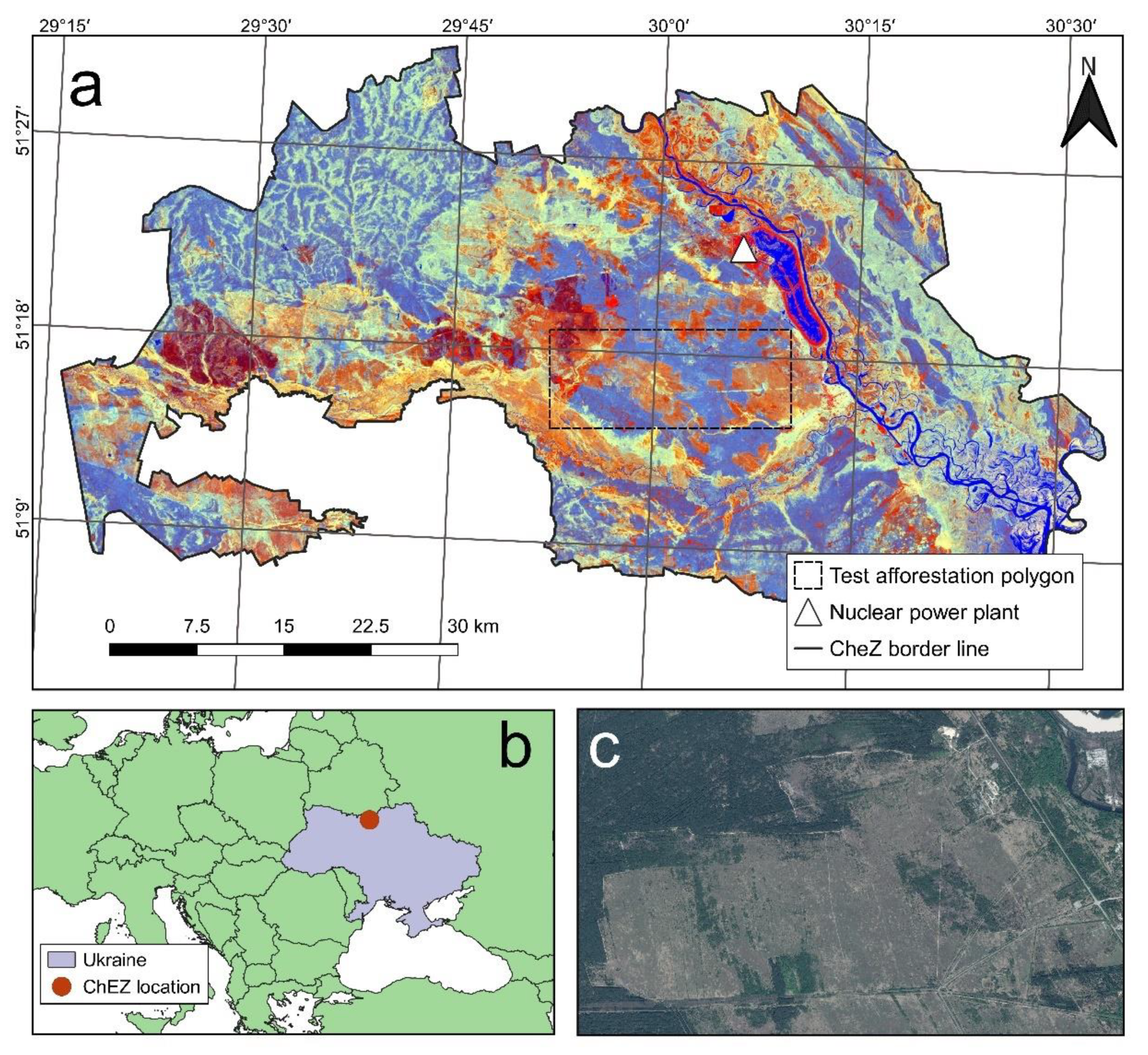
2.1. Study Site

The ChEZ has an area of 2600 km² and is located in northern Ukraine, nearby the border with Belarus (within N 51.084 and N 51.351; E 29.262 and E 30.384). The relief is represented by a plain (i.e., the elevation does not exceed 200 m above sea level). The local climate is continental, with a mean annual temperature of +8.20C and a mean total annual precipitation of 619 mm (for the period 1955–2019). Forests within the ChEZ grow mainly on sod-podzolic soils and are represented either by pure Scots pine planted forests or its mixtures with silver birch, common aspen (Populus tremula L.), black alder (Alnus glutinosa (L.) Gaertn.), and European oak (Quercus robur L.) [13].

To date, the local forests remain largely unmanaged, with limited silvicultural interventions that are confined to the building of assets associated with nuclear waste management infrastructure or to organize firebreaks. In addition, some small portions of the ChEZ forest stands are cut during sanitary loggings (i.e., the clear felling of stands with either infested alive or dead trees up to 200 ha per year). Since the 1986 nuclear disaster, all agricultural activities within the ChEZ have been prohibited and, hence, the abandoned farmlands with the ChEZ have been rapidly afforested. Moreover, large stand-replacing wildfires occurred in that region in the early 1990s, 2015–2016, and 2020. Importantly, the substantial standing deadwood stocks within the severely burned sites have not been treated by any kind of salvage logging since most of these areas (86.7%) are managed as a natural reserve and the deadwood cannot be legally removed, even with the aim of decreasing secondary radionuclide redistribution risks (due to the burning of biomass during wildfires).

2.2. Available Satellite Data

We utilized an open Landsat archive available within the Google Earth Engine (GEE [23]) platform over the time frame of 1986–2020. We applied a standard cloud mask available in GEE to obtain cloud-free mosaics of surface reflectance. The images provided were for the leaf-on season that is typical for woody biota in Ukraine (end of May to the end of September). These multispectral images were the preliminary inputs to building the spectral dataset for use with the LandTrendr (LT) algorithm [17].

The LT algorithm is a well-documented and explored approach to temporally segment an available spectral time series with the main aim of examining changes in biomass and ecosystems in a spatially explicit manner. Typically, it is utilized to map forest disturbances. In addition, by applying a simple linear regression to each pixel in a spatial data set, the LT algorithm allows the spectral value in each pixel to be adjusted according to the trend in the entire time series. That is, this approach is suitable for obtaining spectral data sets with corrected values that are relatively free from noise imputed by clouds, their shadows, and smoke. We applied a standard set of LT hyper-parameters (e.g., the maximum number of segments in the time series for a pixel = 6 and spike threshold = 0.8) fitted by the Normalized Burn Ratio (NBR), which are suitable for detecting the real changes in temperate forests. Based on the adjusted spectral data, we extracted a data set from GEE containing the Normalized Difference Vegetation Index (NDVI), the NBR, the Tasseled Cap Brightness (TCB), the Tasseled Cap Greenness (TCG), and the Tasseled Cap Wetness (TCW) for each year in the 1986–2018 time series. For each annual stack of spectral raster data, we included an elevation data set from the Digital Elevation Model (DEM) provided by the Shuttle Radar Topographic Mission (SRTM, 2000). Thus, the final data set had a 30 m spatial resolution (Figure 1).

We used two historical satellite grayscale images available for the whole ChEZ (SPOT-1; 1987–1988) or for part of it (CORONA, 1967). A Panchromatic Spot-1 image with 10 m spatial resolution was used to manually delineate the forest/non-forest areas with the aim of validating our land cover model for the year 1988. The CORONA image, which is rescaled to a 4 m spatial resolution, was used to manually draw the polygons containing the forests for 1967 within an additional test rectangle polygon located in the central part of the ChEZ (which included both forests and farmlands before the 1986 disaster; see Section 2.4).

2.3. Land Cover Classification and Its Validation

We used a Random Forest (RF [24]) model built on data collected for the year 2017. A training dataset contained 1065 manually interpreted pixels (30 m spatial resolution) with seven assigned land cover classes: “bare soil”; “built-up”; “burned”; “forest”; “grassland”; “water bodies”; and “woodlands”. Pixels were randomly arranged across the ChEZ with a minimum 100 m distance between each one (Figure 2a). This dataset contained 100 pixels from the field observations in the central part of the ChEZ, 900 pixels interpreted using high-resolution images, and 65 pixels manually assigned to the known locations of rare land cover classes such as “water bodies”, “built-up”, and “burned”. The class “forest” was assigned to areas with dense tree cover (covering more than 50% of the pixel area) while the class “woodland” was assigned to areas with sparse forest cover (less than 50% of pixel area under the forest) or shrub cover. Pixels of the ground truth class “burned” were assigned to this class if they were in areas known to be severely disturbed by the massive wildfires that occurred in 2015–2016. The land cover for the pixels from the training sample were manually delineated by using the Google Earth application and the Collect Earth plugin [25]. The RF model was built by using the R-package “randomForest” with standard hyper-parameters (i.e., the number of decision trees in the model ensemble was 500 and the mtry value, which is number of predictors sampled at each decision tree node, was defined as the square root of the total number of model variables). We analyzed the trained RF model by using the out-of-bag overall error rate, user’s accuracies for specific land cover classes, and the relative importance of the variables used in the RF model to predict the land cover classes.

We applied this model to classify each annual stack of LT-fitted spectral values and the elevation from the DEM. In order to validate the model performance in a remote period before 2017 (for which the training data were obtained), we used a dataset of 777 pixels with two assigned classes: “forest” and “non-forest”. We only focused on these two land cover classes instead of the initial seven classes since the available data for land cover delineation were too coarse in resolution to permit different non-forest open landscape types to be properly distinguished (Figure 2b). These pixels were manually delineated by using the aforementioned SPOT-1 image available for 1988 as the “ground-truth” data. We extracted the respective values from our land cover dataset predicted for the same year and reclassified every class, except “forest” to “non-forest”.

We chose an Area Under Curve (AUC) value to assess our model performance. This value, which is calculated for the Receiver Operating Characteristic (ROC), is typically used in a binary classification validation. More specifically, the AUC-ROC can be formulated as Equation (1):

$$AUC={{\displaystyle \int }}_0^{1}TPR\left(FP{R}^{-1}\left(x\right)\right)dx$$

(1)

where TPR is the true positive rate (i.e., the ratio of true positives to the sum of true positives and false negatives) and FPR is the false positive rate (i.e., the ratio of false positives to the sum of true negatives and false positives).

2.4. Analysis of Trends

In addition to providing summary statistics of land cover area dynamics, we calculated the dynamics of the forested area within the aforementioned test rectangular polygon in the central part of the ChEZ. This test site, with an area of 177 km², was chosen to capture the probable change in the ratio of forested and agricultural lands, where these types of land use had taken place prior to the 1986 disaster. The area of forests was obtained from land cover classification maps for the years 2017 and 1988. For the year 1967, we used the CORONA image. The size of this test landscape was chosen so that all available satellite images including the CORONA data were available since the CORONA data do not cover all of the ChEZ area in later years.

In order to observe whether some forest disturbances have resulted in a net forest cover loss in some local areas within the ChEZ, we calculated the net change in the respective land cover class between 1986 and 2020. This calculation was performed for each specific hexagon (with a 3 km side) in a grid drawn for the ChEZ area. A hexagonal grid was chosen to better visualize the summarized changes since using the original 30 m spatial resolution to map change for the entire ChEZ area would be too noisy.

Additionally, we explored the land cover dynamics across three time points in time (1986, 2000, and 2018) by using our land cover maps for these years and a Sankey flowchart diagram. This figure shows how land cover changes through time for each pixel in the data set. In this case, the colors of the three main land cover classes (“forest”, “grassland”, and “woodland”) are defined by the land cover of pixels in 1986 (left part of the diagram) and in 2018 (right part of the diagram), while the year 2000 is presented only by the vertical axis. In order to build this flowchart, we used a data set of 1000 pixels randomly allocated within the mask of abandoned farmlands (Figure 2c). This mask was obtained by manually delineating former agricultural lands by using historical images for 1986. We performed this analysis with the aim of examining the rate of land cover transitions and afforestation within the abandoned farmlands.

3. Results

3.1. Model Training and Validation

The out-of-bag estimate of the overall error for the trained RF model was 22.1%. According to the confusion matrix (

Table 1. Confusion matrix of RF land cover prediction.

Observed/Predicted	Bare Soil	Built-Up	Burned	Forest	Grassland	Water Bodies	Woodland	Classification Error (%)
bare soil	6	1	0	1	2	0	0	40.0
built-up	0	22	1	0	0	1	2	15.3
burned	0	1	43	1	3	0	6	20.4
forest	0	0	2	439	14	0	31	9.7
grassland	1	1	0	16	119	6	55	39.9
water bodies	0	1	0	3	7	19	1	38.7
woodland	0	0	2	28	48	0	182	30.0

), almost all land cover classes achieved 60–70% for the user’s accuracy, while the class “forest” was predicted with the best accuracy (90.4% user’s accuracy) and the class “bare soil” obtained the largest error (60.0% user’s accuracy). The large error that occurred for the land cover class “grassland” was related to the confusion with the “woodland” transitioning class, which is described by highly varying spectral characteristics. The drying landscape of the ChEZ cooling pond (formerly used for the nuclear power plant) may be contributing to the misclassification of “water bodies” as “grasslands” and the rarity of local sandy cover in the ChEZ may be contributing to the respective error for the “bare soil” class. The Tasseled Cap predictors (especially TCW and TCB) together with the DEM elevation were amongst the most important variables for all the land cover classes, while the NDVI and NBR contributed less to the prediction accuracies (Figure 3). The NDVI was better for delineating built-up areas. The predictor’s relative importance for the class “built-up” clearly illustrates how the low number of such training samples had a negative impact on the classification results.

For the year 1988, the land cover classification model applied here achieved a high value of ROC-AUC (0.89, Figure 4). The overall accuracy was quite similar and was 88%. The model incorrectly predicted the “non-forest” class when the true class was “forest” in 17.8% of cases, while the wrong predictions of open landscapes (classified as “forest”) were rarer (4.7%).

3.2. Land Cover Dynamics

Dense forest cover has increased by almost 1.5 times since 1986: from 41.0% up to 59.5% in 2020 (Figure 5). The largest forested proportion of the ChEZ could be observed in 2014, namely 60.4%. This number has been decreasing since then because of the numerous severe wildfires that occurred in 2015–2016 and 2020. While the area of “woodlands” was quite stable during the time frame of this study, there has been a subsequent decrease in the “grassland” area since the late 1980s. Importantly, the area of forest cover is characterized by a constant growth; the exceptions are observed in 1987 when numerous loggings were carried out immediately after the disaster to build necessary infrastructure assets and in 1993 due to salvage logging after a severe wildfire. Such phenomena can be observed even for the first years after the 1986 disaster when abandoned farmlands, which are the main source of natural succession across the timeline, could not contribute to the afforestation process. Maps of land cover for 1986 and 2020 are provided in the Supplementary Materials (Figures S1 and S2).

Most of the ChEZ has experienced net forest cover gain, whilst the respective net loss is reflected by hexagons representing severe wildfires in the early 1990s, the middle 2010s, and in 2020 (Figure 6).

Hexagons where there have been no net forest cover gains compared to 1986 are not all associated with severely burned areas (Figure 6). For example, three hexagons in the southern part of the ChEZ show forest loss due to the flooding of trees and windstorms that occurred in 2016. Regarding burned areas, only the visual cluster of such hexagons located in the southeastern part of the ChEZ represents a large landscape cleared with salvage logging after a severe wildfire occurred in 1993. Other wildfire events (illustrated by dark purple hexagons in the western, northern, and central parts of the ChEZ in Figure 6) were not followed by any human interventions. The yellow hexagons on the map in Figure 6 (with net forest cover gain of up to 450 ha within each one) refer to the abandoned farmlands throughout the ChEZ.

3.3. Forest Transitions

Only a small portion of the land cover class “grassland” was converted to either “forests” or “woodlands” up until the year 2000. However, over the next 18 years, we can observe an increase in the tree density across the abandoned farmlands, which entailed a rapid afforestation and a subsequent change in the land cover mosaics. According to Figure 7, the process of natural succession is hitherto ongoing: an area of “woodlands” is even larger than the dense forest cover in 2018.

Forest cover increased 2.2 times (as of 2017) within the test site in the central part of the ChEZ compared to 1967 (Figure 8). Both a planting of new forest (northern part of the test site; marked by green) and an assisted reforestation of clear-cuts (southwestern part of the test site, marked by red) are visible on the 1988 image: these resulted in a 25% increase compared to 1967. Up to 2017, the most obvious reason for forest cover gain was the succession over the former farmlands, while some new clear-cuts (blue circle) can still be observed in the southwestern part of the test site.

4. Discussion and Conclusions

4.1. Applying Satellite Data to Historical Land Cover Analysis

In this paper, we investigated the suitability of medium spatial resolution Landsat data to map land cover over time. We applied a model trained on novel data (delineated from 2017; very high-resolution data available in Google Earth) and validated the data by using historical data. Panchromatic SPOT-1 images were found to be quite suitable for deriving “forest/non-forest” validation data and this satisfied our aim to examine model performance at a remote point in time (i.e., for 1988). We achieved a good agreement between the model estimates and the empirical data, even considering that the image with a 10 m spatial resolution (i.e., SPOT-1 in this case) cannot be fully harnessed as a source of visual interpretation of “ground-truth” data. However, it is a well known fact that Landsat images robustly capture forest cover dynamics even in fragmented landscapes such as those in Ukraine [26]. Here, we revealed that other land cover classes linked to open landscapes (grasslands and woodlands) can inherit some increased classification errors in the model (Table 1). We assume that this is because of the temporal smoothing when using spectral data fitted by LandTrendr algorithm: emerging additional uncertainty results in misclassification while considering transitioning land cover (grassland to woodland to forest) with similarly specific spectral values.

Typically, by utilizing several images or digitized historical maps available at specific points of time (with the period between the acquisitions ranging from 5 to10 to 50 years, [27,28]), it is possible to capture land cover dynamics with a sufficient degree of accuracy and adequacy. Moreover, temporally segmented Landsat time series can support a smoother, continuous, and more error-free background for the comprehensive analysis of forest transitions under rapid natural successions. In this regard, the LandTrendr algorithm allows not only forest disturbances and the subsequent biomass restoration to be mapped but it also allows the monitoring of afforestation processes within landscapes that were not previously covered by woody vegetation.

We have shown that our classification model has captured the main forest cover loss driven by severe wildfires (Figure 4 and Figure 5). Substantial forested areas (>800 km²) have been reported to be burned according to Beresford et al. (2021 [16]), but there were only 143 km² of the land cover class “burned” in our remote sensing-based predictions (Figure S2). However, this mask of “burned” areas coincides well with a mapped delta NBR (a net change of NBR between 2020 and 2019 as a typically used indicator of wildfire and other disturbance severities [15]) shown in Figure S3. Only a delta NBR larger than 100 was mapped, i.e., the mean delta NBR in this map was 300, while the delta NBR filtered by land cover class “burned” was only 400. Additionally, ~290 km² of the ChEZ experienced a 2020 NBR drop in the total NBR values larger than 50, compared to 2019. Therefore, our model captured only severely disturbed woody communities, namely stand replacing. It is important to mention that the LandTrendr algorithm smooths spectral trajectories in temporal trends [17] and the data for 2020, as the last point in the time series, might be affected by this feature.

Compared to global forest cover datasets of different spatial and temporal resolutions, our classification model better captured the forest cover gain dynamics for the area of the ChEZ. Global Forest Change (GFC [1]) data are frequently applied to examine forest cover loss and gain after 2000. Setting the canopy closure threshold for the GFC data to 40%, we show in Figure 9 that forest cover loss values (2000–2020) match quite well with our ChEZ land cover product at the same spatial (30 m) and temporal resolution.

However, while forest cover loss values were quite similar (233 km² defined by the GFC vs. 174 km² defined by our RF model), the GFC dataset underestimated the forest cover gain during the last 20 years by 6.3 times (78 km² defined by GFC vs. 490 km² as found by our land cover model). The insufficient capability of the GFC data to fully capture the forest cover gain dynamics in Ukraine has already been reported [26]. Similar conclusions can be made when our local model and the global Historic Land Dynamics Assessment (HILDA [29]) dataset are compared (Figure 10).

The two maps in Figure 10 do not include the year 2020 when severe wildfires occurred and, similar to the GFC, they represent forest cover loss in the central and western parts of the ChEZ associated with burned areas in 2015–2016. In addition, the HILDA dataset can be used to visualize additional forest cover loss in the south-eastern part of the ChEZ that occurred before 1986. However, similar to the GFC, it failed to reflect the proper forest cover gain with an underestimation compared to our model of almost 10 times. Therefore, only local products can realistically reproduce afforestation processes, although global products are still good for mapping deforestation.

4.2. Net Afforestation in the ChEZ

Through our analysis, we revealed that natural forests within the ChEZ have totally compensated for any forest cover loss from disturbances (Figure 6), despite the fact that disturbances, i.e., mainly wildfires, have been frequently reported [14,15]. These findings fill the gaps between the sparse sources of data on the forest covers in ChEZ, which were typically quantified by only using conventional forest surveys conducted in 2006 and 2016. The net forest gain has literally converted the area of the ChEZ into a system of landscapes dominated by woody vegetation (Figure 5). The trend in the land cover class “woodlands” has been stable over time: The annual area values have remained similar because of simultaneous transitions, i.e., “grassland ≥ woodland” and “woodland ≥ forest”. Meanwhile, some declines can be observed during the last few years, which are clearly linked to the severe wildfires that occurred both in dense and sparse woody communities in 2015–2016. However, this does not really reflect the possible catastrophic situation in which wildfires dynamically shape land cover [16] within abandoned fields, as wildfires are now occurring with an almost annual frequency. Disregarding the ongoing negative consequences of droughts on forests in the temperate zone [30], the forest covers in the ChEZ have not generally decreased.

We have found that the transition of open landscapes (Figure 7) to somewhat woody communities within former farmlands (as revealed by remote sensing techniques) has taken at least 14 years to occur (i.e., from 1986 to 2000). However, even pioneer tree species (such as silver birch and common aspen) did not create a dense forest cover within most of the 900 m² pixels up until the year 2000, i.e., only 39 pixels out of a sample of 1000 had dense forest cover. During the last 18 years, the “woodlands” fraction has become significantly larger. Such continuous afforestation can be explained by the fact that even during the last decade, the dominant tree species has been Scots pine, which possesses lower growth rates than the aforementioned broadleaved species. This past management legacy is important for understanding the current situation, as young conifers with dense herbaceous ground floors are highly prone to rapidly spreading severe wildfires.

4.3. Implications

Conventional but still balanced forest management in Soviet times (based on full replanting of large clear-cuts and continuous artificial afforestation, Figure 7) has restored the forest cover in the post-war period and kept it stable until the collapse of the USSR [31]. Additionally, the cessation of crop production carried out within relatively small-populated regions with low-fertile soils [7,10] has resulted in projections of uncontrolled afforestation throughout northern Ukraine and, specifically, in the ChEZ. This uncontrolled afforestation on abandoned farmlands is frequently considered as a robust source of official forest cover “gain”, which is the main target of Ukraine’s forest policy due to insufficient state financial support for a wide afforestation program (by planting trees [5]). However, unlike the non-protected landscapes outside of the ChEZ, such forests cannot be managed in a traditional way. That is, policy makers should consider, with caution, the fact that these new forests do not really provide a stable cover, a carbon sink, or woody habitats for certain ChEZ fauna.

By contrast, the neighboring countries of Ukraine, which share similar environmental conditions and dominant tree species, typically consider uncontrolled afforestation as a threat to open natural landscapes such as meadows [32,33]. In Poland, such forests are properly monitored by utilizing satellite and laser scanning data (e.g., [34]). It is crucial to consider the woody succession, focusing not on the natural meadows and steppes with an important herbaceous flora but rather on typical farmlands abandoned immediately after the socialist era. Such phenomenon should be accounted for and managed with respect to both the public and the scientific community. Yet, researchers recommend preventing such afforestation as former agricultural fields can transition instead to natural fields [9]. Importantly, the area of indigenous meadows and steppes in Ukraine is rather small. Therefore, the importance of widespread and rapid afforestation within protected areas of the ChEZ is questionable.

At the same time, it is worth mentioning that the ChEZ performs a number of protective functions, where the basic one is the restriction of the spatial migration of radionuclides outside of the contaminated territories. In this context, forest and shrub ecosystems have greater advantages over grassy landscapes because woody vegetation reduces the lateral migration of unnatural radioisotopes in the upper soil layers more efficiently. Currently, ¹³⁷Cs and ⁹⁰Sr contribute the largest share in the formation of the absorbed dose rate of organisms in the ChEZ (i.e., two biologically mobile radionuclides that are easily incorporated into biogenic fluxes). If the main depot for these radionuclides in grassland ecosystems [35] is only soil, then forests and woodlands can accumulate significant amounts of ¹³⁷Cs and ⁹⁰Sr in tree trunks and litter (i.e., up to 50%) [12]. In this regard, wildfires in forest ecosystems are more dangerous for some aspects of radionuclide transfer; this applies not only in the form of aerosols in the air but also due to wash off from post-fire materials into running water basins if they are compared to meadow wildfires [14,15,36]. However, the aforementioned radionuclides have a half-life of about 30 years compared to most isotopes of trans-uranium elements, which suggests that in 60–90 years, it will be possible to harvest wood products in forest areas represented by young stands without violating the current hygienic standards of Ukraine. These stands are characterized by insignificant contamination of tree trunks and are not included in the ChEZ core reserve areas. Therefore, the Chernobyl forests can be grown as a future reserve of probable wood products for economic purposes while simultaneously ensuring the barrier function near highly contaminated territories.

We conclude that local forests of ChEZ are not sufficiently resilient to be left totally untouched since the social demand to keep radionuclides’ depos stable hitherto prevails. The main purpose of these ecosystems should be thought in terms research and preservation goals, with limited silvicultural interventions to decrease fuel stocks and possible options for timber production in certain future. Time series of freely available satellite data should be continuously harnessed by ChEZ managers and researchers as the efficient tool for capturing annual land cover change and for correctly adjusting local planning activities.

References

1. Hansen, M.C.; Potapov, P.V.; Moore, R.; Hancher, M.; Turubanova, S.A.; Tyukavina, A.; Thau, D.; Stehman, V.; Goetz, S.J.; Loveland, T.R.; et al. High-resolution global maps of 21st-century forest cover change. Science 2013, 342, 850–853. [Google Scholar] [CrossRef] [Green Version]
2. Seidl, R.; Thom, D.; Kautz, M.; Martin-Benito, D.; Peltoniemi, M.; Vacchiano, G.; Wild, J.; Ascoli, D.; Petr, M.; Honkaniemi, J.; et al. Forest disturbances under climate change. Nat. Clim. Chang. 2017, 7, 395–402. [Google Scholar] [CrossRef] [Green Version]
3. Bastin, J.-F.; Finegold, Y.; Garcia, C.; Mollicone, D.; Rezende, M.; Routh, D.; Zohner, C.M.; Crowther, T.W. The global tree restoration potential. Science 2019, 365, 76–79. [Google Scholar] [CrossRef] [PubMed]
4. Doelman, J.C.; Stehfest, E.; van Vuuren, D.P.; Tebeau, A.; Hof, A.F.; Braakhekke, M.C.; Gernaat, D.E.H.J.; van der Berg, M.; van Zeist, W.-J.; Daioglou, V.; et al. Afforestation for climate change mitigation: Potentials, risks and trade-offs. Glob. Chang. Biol. 2019, 26, 1576–1591. [Google Scholar] [CrossRef]
5. Shvidenko, A.; Buksha, I.; Krakovska, S.; Lakyda, P. Vulnerability of Ukrainian Forests to Climate Change. Sustainability 2017, 9, 1152. [Google Scholar] [CrossRef] [Green Version]
6. Thom, D.; Rammer, W.; Garstenauer, R.; Seidl, R. Legacies of past land use have a stronger effect on forest carbon exchange than future climate change in a temperate forest landscape. Biogeosciences 2018, 15, 5699–5713. [Google Scholar] [CrossRef] [Green Version]
7. Bilous, A.; Myroniuk, V.; Holiaka, D.; Bilous, S.; See, L.; Schepaschenko, D. Mapping growing stock volume and forest live biomass: A case study of the Polissya region of Ukraine. Environ. Res. Lett. 2017, 12, e105001. [Google Scholar] [CrossRef] [Green Version]
8. Kuemmerle, T.; Olofsson, P.; Chaskovskyy, O.; Baumann, M.; Ostapowicz, K.; Woodcock, C.E.; Houghton, R.A.; Hostert, P.; Keeton, W.S.; Radeloff, W. Post-soviet farmland abandonment, forest recovery, and carbon sequestration in western Ukraine. Glob. Chang. Biol. 2011, 17, 1335–1349. [Google Scholar] [CrossRef]
9. Osinska-Skotak, K.; Radecka, A.; Piorkowski, H.; Michalska-Hejduk, D.; Kopec, D.; Tokarska-Guzik, B.; Ostrowski, W.; Kania, A.; Niedzielko, J. Mapping Succession in Non-Forest Habitats by Means of Remote Sensing: Is the Data Acquisition Time Critical for Species Discrimination? Remote Sens. 2019, 11, 269. [Google Scholar] [CrossRef] [Green Version]
10. Hostert, P.; Kuemmerle, T.; Prishchepov, A.; Sieber, A.; Lambin, E.F.; Radeloff, V.C. Rapid land use change after socio-economic disturbances: The collapse of Soviet Union versus Chernobyl. Environ. Res. Lett. 2011, 6, 045201. [Google Scholar] [CrossRef]
11. Lesiv, M.; Shvidenko, A.; Schepaschenko, D.; See, L.; Fritz, S. A spatial assessment of the carbon budget for Ukraine. Mitig. Adapt. Strateg. Glob. Chang. 2019, 24, 985–1006. [Google Scholar] [CrossRef] [Green Version]
12. Yoschenko, V.; Ohcubo, T.; Kashparov, V. Radioactive contaminated forests in Fukushima and Chernobyl. J. For. Res. 2017, 21. [Google Scholar] [CrossRef]
13. Matsala, M.; Bilous, A.; Myroniu, V.; Diachuk, P.; Burianchuk, M.; Zadorozhniuk, R. Natural forest regeneration in Chernobyl Exclusion Zone: Predictive mapping and model diagnostics. Scand. J. For. Res. 2021, 36, 164–176. [Google Scholar] [CrossRef]
14. Evangeliou, N.; Zibtsev, S.; Myroniuk, V.; Zhurba, M.; Hamburger, T.; Stohl, A.; Balkanski, Y.; Paugam, R.; Mousseau, T.A.; Moller, A.P.; et al. Resuspension and atmospheric transport of radionuclides due to wildfires near Chernobyl Nuclear Power Plant in 2015: An impact assessment. Sci. Rep. 2016, 6, 26062. [Google Scholar] [CrossRef] [PubMed]
15. Ager, A.A.; Lasko, R.; Myroniuk, V.; Zibtsev, S.; Day, M.A.; Usenia, U.; Bogomolov, V.; Kovalets, I.; Evers, C.R. The wildfire problem in areas contaminated by the Chernobyl disaster. Sci. Total Environ. 2019, 696, 133954. [Google Scholar] [CrossRef]
16. Beresford, N.; Barnett, C.L.; Gashchak, S.; Kashparov, V.; Kirieiev, S.I.; Levchuk, S.; Morozova, V.; Smith, J.T.; Wood, M.D. Wildfires in the Chornobyl Exclusion Zone-risks and consequences. Integr. Environ. Assess. Manag. 2021. [Google Scholar] [CrossRef]
17. Kennedy, R.; Yang, Z.; Cohen, W. Detecting trends in forest disturbance and recovery using yearly Landsat time series: 1. LandTrendr—Temporal segmentation algorithms. Remote Sens. Environ. 2010, 114, 2897–2910. [Google Scholar] [CrossRef]
18. Kozubov, G.; Taskaev, A. Radiological and Radioecological Studies of Woody Plants; Nauka: St. Petersburg, Russia, 1994. (In Russian) [Google Scholar]
19. Holiaka, D.; Fesenko, S.; Kashparov, V.; Protsak, V.; Levchuk, S.; Holiaka, M. Effects of radiation on radial growth of Scots pine in areas highly affected by the Chernobyl accident. J. Environ. Radioact. 2020, 222, 106320. [Google Scholar] [CrossRef]
20. Kukarskih, V.V.; Modorov, M.V.; Devi, N.M.; Mikhailovskaya, L.N.; Shimalina, N.S.; Pozolotina, V.N. Radial growth of Pinus sylvestris in the East Ural Radioactive Trace (EURT): Climate and ionizing radiation. Sci. Total Environ. 2021, 781, 146827. [Google Scholar] [CrossRef]
21. Geraskin, S.A.; Fesenko, S.V.; Alexakhin, R.M. Effects of non-human species irradiation after the Chernobyl NPP accident. Environ. Int. 2008, 34, 880–897. [Google Scholar] [CrossRef] [PubMed]
22. Yoschenko, V.; Kashparov, V.; Melnychuk, M.; Levchuk, S.; Bondar, Y.; Lazarev, M.; Yoschenko, M.; Farfan, E.; Jannik, T. Chronic irradiation of Scots pine trees (Pinus sylvestris) in the Chernobyl Exclusion Zone: Dosimetry and radiobiological effects. Health Phys. 2011, 101, 393–408. [Google Scholar] [CrossRef] [PubMed] [Green Version]
23. Gorelick, N.; Hancher, M.; Dixon, M.; Ilyushchenko, S.; Thau, D.; Moore, R. Google Earth Engine: Planetary-scale geospatial analysis for everyone. Remote Sens. Environ. 2017, 202, 18–27. [Google Scholar] [CrossRef]
24. Breiman, L. Random Forests. Mach. Learn. 2001, 45, 5–32. [Google Scholar] [CrossRef] [Green Version]
25. Bey, A.; Díaz, A.S.-P.; Maniatis, D.; Marchi, G.; Mollicone, D.; Ricci, S.; Bastin, J.-F.; Moore, R.; Federici, S.; Rezende, M.; et al. Collect Earth: Land use and land cover assessment through augmented visual interpretation. Remote Sens. 2016, 8, 807. [Google Scholar] [CrossRef] [Green Version]
26. Myroniuk, V.; Kutia, M.; Sarkissian, A.J.; Bilous, A.; Liu, S. Regional-Scale Forest Mapping Over Fragmented Landscapes Using Global Forest Products and Landsat Time Series Classification. Remote Sens. 2020, 12, 187. [Google Scholar] [CrossRef] [Green Version]
27. Lieskovsky, J.; Kaim, D.; Balasz, P.; Boltiziar, M.; Chmiel, M.; Grabska, E.; Kiraly, G.; Konkoly-Gyuro, E.; Kozak, J.; Antalova, K.; et al. Historical land use dataset of the Carpathian region (1819–1980). J. Maps 2018, 14, 644–651. [Google Scholar] [CrossRef] [Green Version]
28. Shen, W.; Li, M.; Huang, C.; Tao, X.; Li, S.; Wei, A. Mapping annual forest change due to afforestation in Guangdong Province of China using active and passive remote sensing data. Remote Sens. 2019, 11, 490. [Google Scholar] [CrossRef] [Green Version]
29. Winkler, K.; Fuchs, R.; Rounsevell, M.; Herold, M. Global land use changes are four times greater than previously estimated. Nat. Commun. 2021, 12, 2501. [Google Scholar] [CrossRef]
30. Senf, C.; Buras, A.; Zang, C.S.; Rammig, A.; Seidl, R. Excess forest mortality is consistently linked to drought across Europe. Nat. Commun. 2020, 11, 6200. [Google Scholar] [CrossRef] [PubMed]
31. Nilsson, S.; Sallnas, O.; Hugosson, M.; Shvidenko, A. The Forest Resources of the Former European USSR; The Parthenon Published Group Limited: Canrforth, UK, 1992; p. 403. [Google Scholar]
32. Janus, J.; Bozek, P. Using ALS data to estimate afforestation and secondary forest succession on agricultural areas: An approach to improve the understanding of land abandonment cases. Appl. Geogr. 2018, 97, 128–141. [Google Scholar] [CrossRef]
33. Sackov, I.; Barka, I.; Bucha, T. Mapping aboveground woody biomass on abandoned agricultural land based on airborne laser scanning data. Remote Sens. 2020, 12, 4189. [Google Scholar] [CrossRef]
34. Janus, J.; Bozek, P. Land abandonment in Poland after the collapse of socialism: Over a quarter of a century of increasing tree cover on agricultural land. Ecol. Eng. 2019, 138, 106–117. [Google Scholar] [CrossRef]
35. Beresford, N.A.; Scott, E.M.; Copplestone, D. Field effects studies in the Chernobyl Exclusion Zone: Lessons to be learnt. J. Environ. Radioact. 2020, 211, 105893. [Google Scholar] [CrossRef] [PubMed]
36. Igarashi, Y.; Onda, Y.; Wakiyama, Y.; Konoplev, A.; Zheleznyak, M.; Lisovyi, H.; Laptev, G.; Damiyanovich, V.; Samoilov, D.; Nanba, K.; et al. Impact of wildfire on 137Cs and 90Sr wash-off in heavily contaminated forests in the Chernobyl exclusion zone. Environ. Pollut. 2020, 259, 113764. [Google Scholar] [CrossRef]
Figure 1. Study area: (a) the Chernobyl Exclusion Zone (ChEZ) overlaid with a false-color Tasseled Cap composite (TCB, TCG, TCW); (b) the location of the ChEZ in Europe; and (c) an example of a very high-resolution (2017) image from Google Earth for a test afforestation polygon.
Forests 12 01024 g001
Figure 2. Data sets: (a) interpreted land cover training data for the classification model; (b) validation data of forest/non-forest cover in 1988; and (c) a collection of pixels within abandoned farmlands for examining the land cover transitions.
Forests 12 01024 g002
Figure 3. Relative importance of RF model variables for predicting land cover classes for the year 2017.
Forests 12 01024 g003
Figure 4. (a) A confusion matrix of the binary model validation (for the year 1988) and (b) the ROC-AUC graph.
Forests 12 01024 g004
Figure 5. Land cover dynamics (1986–2020) predicted by the classification model applied to the LT-fitted spectral data set.
Forests 12 01024 g005
Figure 6. Forest cover gain between 1986 and 2020. The color gradient is quantile: only dark blue hexagons refer to a forest cover loss, while the gain is represented by other colors.
Forests 12 01024 g006
Figure 7. Land cover transitions within abandoned farmlands.
Forests 12 01024 g007
Figure 8. Change in forest cover within the test site in the central part of the ChEZ. The green circle refers to artificial forest planting, the red circle to regrown clear-cuts up to 1988 and the blue circle refers to new clear-cuts that have appeared up until 2017.
Forests 12 01024 g008
Figure 9. (a) Global Forest Change (GFC [1]) data vs. (b) our forest cover change product for the period 2000–2020.
Forests 12 01024 g009
Figure 10. (a) Historic Land Dynamics Assessment (HILDA [29]) forest cover change data for the period 1960–2019 vs. (b) our forest cover change product for the period 1986–2019. The spatial resolution of both maps is 1 km2.
Forests 12 01024 g010