Article

The Potential Distribution of Juniperus rigida Sieb. et Zucc. Vary Diversely in China under the Stringent and High GHG Emission Scenarios Combined Bioclimatic, Soil, and Topographic Factors

1
College of Forestry, Northwest A & F University, Yangling, Xianyang 712100, China
2
Shaanxi Key Laboratory of Economic Plant Resources Development and Utilization, Yangling, Xianyang 712100, China
*
Author to whom correspondence should be addressed.
Forests 2021, 12(9), 1140; https://doi.org/10.3390/f12091140
Submission received: 16 July 2021 / Revised: 19 August 2021 / Accepted: 20 August 2021 / Published: 24 August 2021
(This article belongs to the Section Forest Ecology and Management)

Abstract

:
Global warming poses an enormous threat to particular species with shifts to their suitable habitat. Juniperus rigida Sieb. et Zucc., an endemic species to East Asia and a pioneer species in the Loess plateau region, is endangered because of the shrinking and scattered habitat threatened by climate change. For the sake of analyzing the impact of climate warming on its possible habitat, we herein projected the current and future potential habitats of J. rigida in China and comparatively analyzed the ecological habitat changes in three main distribution regions. There were 110 specimen records of J. rigida collected across China and 22 environmental datasets, including bioclimatic variables and soil and topographical factors, selected by the Pearson Correlation Coefficient. The MaxEnt model based on specimen presence and environmental factors was used for projecting the potential habitats of J. rigida in China in the 2050s and the 2070s of RCP 2.6 and RCP 8.5 scenarios. The results indicated an excellence model performance with the average value of the area under curve (AUC) is 0.928. The mean temperature of the driest quarter (MTDq) and the temperature annual range (TAR) provided important contributions to the potential distribution of J. rigida. There were three main distribution areas in China, the Xinjiang region, the Loess-Inner Mongolian Plateau region, and the Changbai Mountain region. The distribution increased overall in area under RCP 2.6 and decreased for RCP 8.5. The mean altitude of the core distribution shifted upward in general under both scenarios. The Loess–Inner Mongolian Plateau region is the biggest distribution, encompassing ca. 61.39 × 10⁴ km2 (86.87 × 10⁴ km2 in China). The region threatened most by climate change is located in the Changbai Mountain distribution, with the centroid of the cord suitable habitat migrating southwest about 227.47 and 260.32 km under RCP 2.6 and RCP 8.5 by the 2070s. In summary, these findings provided a well-grounded understanding of the effect of climate change on ecological distribution and furnished theory evidence for the protection, management, and sustainable use of J. rigida.

Graphical Abstract

1. Introduction

Greenhouse gas (GHG) emissions have led to global warming, which has now become a global issue [1]. It was projected that, by the end of the 21st century (2081–2100), relative to 1986–2005 with the reason of increasing GHG emission during the industrial age, the global average surface temperature is likely to increase by 0.3–1.7 °C under the RCP 2.6 scenario, 1.1–2.6 °C under the RCP 4.5 scenario, and could be 1.4–3.1 °C under the RCP 6.0 scenario and 2.6–4.8 °C under the RCP 8.5 scenario [2]. Changing climatic conditions have had a profound impact on the distribution range of species, placing the global ecological environment under inconceivable pressure [3,4], determining the viability and conservation potential of various species [5], and altering species’ dominance, survival, migration, and community structure [6]. Consequently, some species will either shift their distributions or be extinguished as a result of further climate change in the future [7].
The ecological niche was defined by Grinnell [8] in 1917 and Elton [9] in 1927, respectively. Hutchinson [10] proposed the hypervolume niche and defined it as the set of all variables that allow species to exist indefinitely in 1957. There are numerous established models, such as Bioclim [11], DOMAIN [12], GARP [13], and MaxEnt [14], to simulate ecological requirements and distribution areas of species based on niche theory. Among these models, MaxEnt has been widely used owing to its advantages over other approaches, for instance, stable operation result, high simulation precision, and so on [15]. These features stand out in cases involving incomplete known geographical distribution data and the relevant environment variables that affect distributions [16,17].
The Juniperus rigida Sieb. et Zucc., Cupressaceae plant with the characteristics of hardiness, drought resistance, and soil and water conservation, is endemic to East Asia. The species is mainly distributed in cold temperate regions of the northern hemisphere, North and Northeastern China, Korea, and Japan. It is the key protected plant and almost endangered species now in China [18]. It is climate warming and its biological characteristics that shrink and fragment its distributions [19]. Therefore, it is meaningful to figure out the impact of climate change on its distribution in terms of formulating effective conservation strategies for J. rigida.
Here, we used MaxEnt to project the potential distribution of Juniperus rigida Sieb. et Zucc. under current and future climate scenarios and to analyze the change of potential distribution in three main distributions across China. The specific objectives are (1) to project the potential distribution areas of J. rigida across China, (2) to assess the important variables affecting the distribution of J. rigida, and (3) to analyze the rules of the area change and the centroid shift in the three main distributions.

2. Materials and Methods

2.1. Collection and Processing of Species Distribution Data

The current occurrence records of Juniperus rigida Sieb. et Zucc. throughout China derived from the Global Biodiversity Information Facility (GBIF, https://www.gbif.org/, accessed on 20 November 2020), the Chinese Virtual Herbarium databases (CVH, http://v5.cvh.org.cn/, accessed on 28 November 2020) and Specimen Resources Sharing Platform for Education (http://mnh.scu.edu.cn/, accessed on 5 December 2020). We obtained 557 occurrence records. The duplicates and those that lacked exact geo-coordinate record points were not taken into account. Finally, there remained 110 occurrence points that could carry out the MaxEnt model program and develop the distribution map integrated the topographic information with the ArcGIS 10.2 (Esri, Redlands, CA, USA) (Figure 1). Those records were divided into three regions, which will be emphasized.

2.2. Collection and Selection Climate, Soil, and Topographical Data

The current period (1950–2000) bioclimatic variables with 30 arc seconds (approximately 1 km2) spatial resolution were downloaded from the WorldClim-Global Climate Database (http://worldclim.org/, accessed on 11 October 2020). They represented annual or seasonality trends and extreme or limiting environmental factors [20] and were the most crucial variables affecting potential species distribution [21].
Future period (2050s and 2070s) bioclimatic variables with the same geographical accuracy and variable names with current bioclimatic variables were extrapolated by a global circulation model. There were four representative concentration pathways (RCPs) established in the 5th report of the IPCC (Intergovernmental Panel on Climate Change) [22], which means the future climate change was diverse and uncertain. RCP 2.6 was a lower greenhouse gas emission scenario and was paid widespread attention because it could achieve the goal of no more than 2 °C of global warming by 2100 relative to pre-industrial levels [23,24]. Holding the increase in the global average temperature below 2 °C above pre-industrial levels and striving to limit the increase to 1.5 °C above pre-industrial levels is the common goal for all countries in the world by reducing greenhouse gas emissions [25]. RCP 8.5 was a robust GHG emission scenario without additional efforts to constrain emissions, which posed a high risk of abrupt and irreversible regional-scale change in the composition, structure, and function of ecosystems [22]. Therefore, we chose RCP 2.6 and RCP 8.5 under BCC-CSM1-1 climate change modeling, an efficient global climate tool for the simulation of future climatic conditions that performs perfectly for the simulation of precipitation and temperature in the Chinese region [26,27]. There were two periods for model projection; the 2050s and 2070s represent 2041–2060 and 2061–2080, respectively.
Insolation duration and relative humidity were provided by the China Meteorological Data Service Center (CMDC, http://data.cma.cn/en, accessed on 25 October 2020). These data were observed by 613 data and basic ground meteorological observation stations in China, and the mean value of each observation station was calculated during 1951~2000 to develop the relevant lay using kriging interpolation with the software of ArcGIS 10.2 (Esri, Redlands, CA, USA). The China Soil Map-Based Harmonized World Soil Database (v1.1) was derived from the Cold and Dry Area Scientific Data Center (http://westdc.westgis.ac.cn, accessed on 10 September 2020). The aspect and slope variables were generated based on the altitude dataset obtained from ISDSP (http://datamirror.csdb.cn/, accessed on 13 September 2020).
All the data were processed with the same spatial resolution as the climate data. Many of the environmental variables that are spatially correlated can result in model over-fitting [16]. We used the Pearson correlation coefficient to examine the multi-collinearity of variables and removed one or more highly correlated environmental factors if p > 0.8. Ultimately, we retained 22 factors for modeling (Table 1) and converted the data to the ASCII format.

2.3. Model Establishment and Accuracy Test

The maximum entropy model (MaxEnt, version 3.4.1) is available freely online (http://www.cs.princeton.edu/wschapire/Maxent/, accessed on 4 June 2020). All the variables selected were imported into the model to project the potential distribution. The current climate data were replaced with the future climate data when the potential distribution is projected in the future climate scenario, while the soil and terrain data remain unchanged. The Akaike information criterion (AICc) visually manifest the optimal combination for two parameters, feature classes and regularization multiplier, which were of great importance to the fitting degree of MaxEnt [28]. We ran the model with default values of the two parameters, and the good performance had been verified [29].
The fitted model precision was evaluated based on the area under the receiver operating characteristic curve (AUC-ROC), with the criterion of values for AUC > 0.9 representing more adequate fit [30] by 10 fold cross-validation. The receiver operating characteristic curve (ROC) graphically displayed the performance of the model [31]. The output was in cloglog format with the probability (0~1) of the presence of J. rigida in each grid of 30 arc-seconds resolution. The maximum training sensitivity plus specificity criterion we utilized had been recognized as one of the best threshold (TH) selection methods on account of the optimized specificity and sensitivity using training data [32]. The maximum number of background points and iterations were set to 10,000 and 3000, respectively, which ensured that the model had adequate time to converge, while the other parameters defaulted according to the MaxEnt Tutorial [33].

2.4. Potential Habitat Assessment

We classified the distribution into 4 levels, unsuitable (<TH), general (TH~0.5), moderate (0.5~0.8), and core (0.8~1), and illustrated them in pictures, according to the suitable indices for each climate scenario provided by MaxEnt.
The distribution changes in the future climate scenarios were in three patterns, new, disappeared, and unchanged, compared with current habitat. To illustrate the change in future scenarios, we replaced the continuous probability value with the discrete binary and recalculated the grid value using the following formula. The grids with a probability above the threshold were assigned to 1 representing suitability habitats, and the others to 0 representing unsuitability habitats.
It can be calculated using the formula following.
X = GCC × 2 + GCF, X∈(0, 1, 2, 3)
where GCC was the grid code under the current climate, GCF was the grid code under the future climate. When X = 0 represented the unsuitable distribution under current and future climate, X = 1 represented the new distribution under future climate, X = 2 represented the disappeared distribution under future climate, and X = 3 represented the unchanged distribution.

2.5. The Shift of the Core Distribution Centroid

We assumed the core distribution area of Juniperus rigida Sieb. et Zucc. to a single centroid point that could be calculated with the help of the SDM tool-box, a type of python-based GIS software. The core distribution is the geospatially highly suitable area for J. rigida. The magnitude and direction of distribution area change were analyzed more clearly by comparing the centroid point position under the current and future climate.

3. Results

3.1. Model Evaluation and Important Variables

The MaxEnt model for Juniperus rigida Sieb. et Zucc. generated excellent evaluations under the given parameter setting conditions, with the average test AUC value of 0.928 ± 0.025 for the 10 times replicate runs. Making a comprehensive analysis of the percent contribution and permutation importance of all predictive variables provided by the MaxEnt result, those variables, slope (Slo), altitude (Alt), mean temperature of driest quarter (MTDq), and temperature annual range (TAR), were the domain environmental factors with higher percent of contribution relative to other variables. Furthermore, annual mean temperature (AMT), annual precipitation (AP), temperature seasonality (TS), and precipitation of wettest month (PWm) made a greater contribution to the permutation importance. The cumulative contributions of these factors hit a value as high as 76.8% (Table 1).

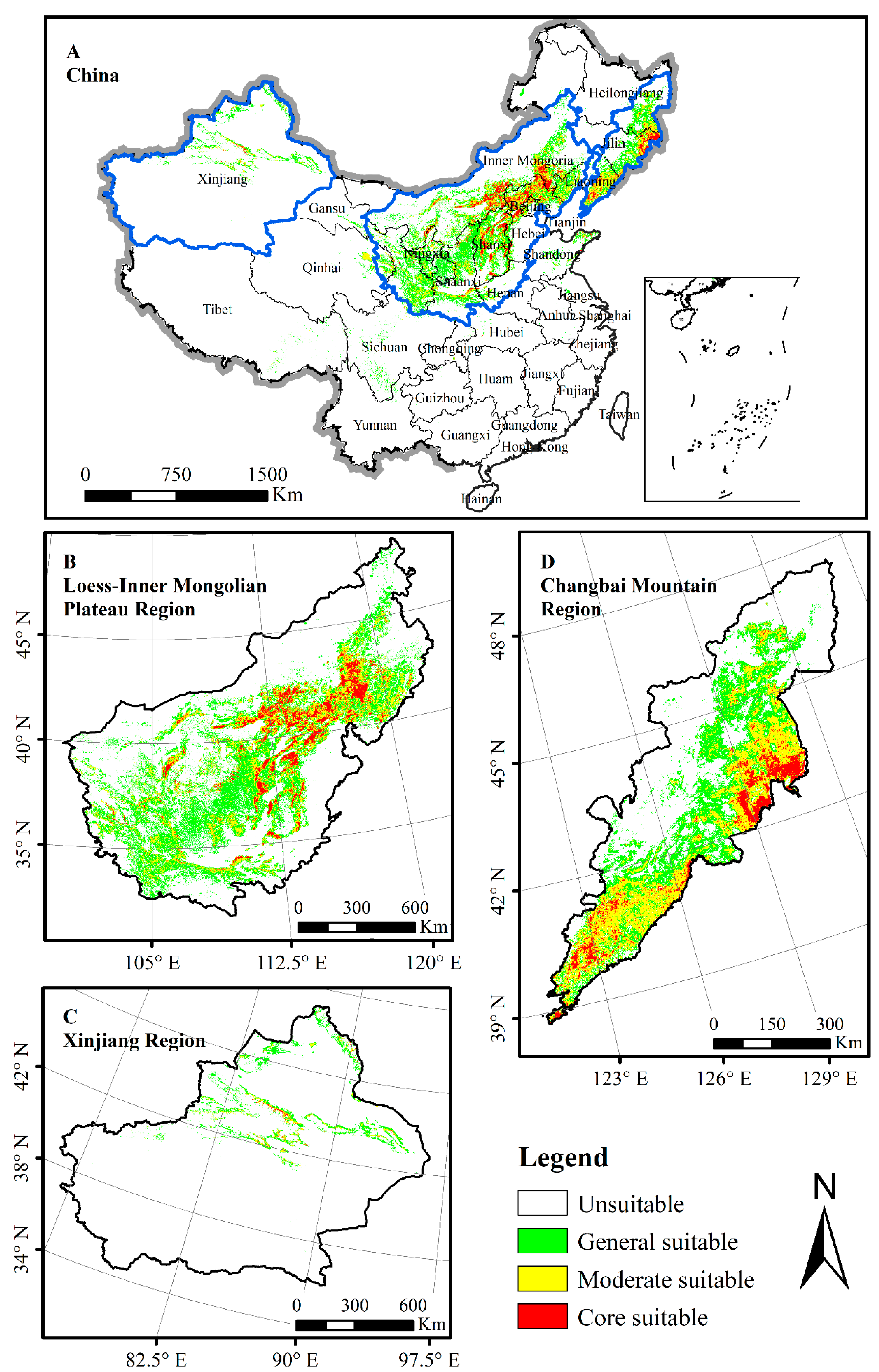
3.2. The Potential Distribution of J. rigida under the Current Climate

The suitability was classified into four levels and was shown in Figure 2A. The simulated suitable habitat under the current climate scenario was mainly distributed in three regions, the Xinjiang region, the Loess-Inner Mongolian Plateau region, and the Changbai Mountain region, which were illustrated in Figure 2B–D, respectively.
The national ecological suitable area was 86.87 × 10⁴ km2 and the core suitable area was 10.13 × 10⁴ km2 accounting for 11.66% of the total potential habitat (Table 2). The suitable distribution of the Loess-Inner Mongolia plateau region was larger than other two regions, reaching 61.39 km2. The core ecological suitable area in this region accounted for 13.04% of the total suitable area, and the percentage was higher than the national average.
The Xingjiang region had the smallest ecological suitable area, with the area size of 5.65 km2. The proportions of the moderate and core suitable habitat were 19.25% and 3.89% respectively, which were significantly lower than the national average.

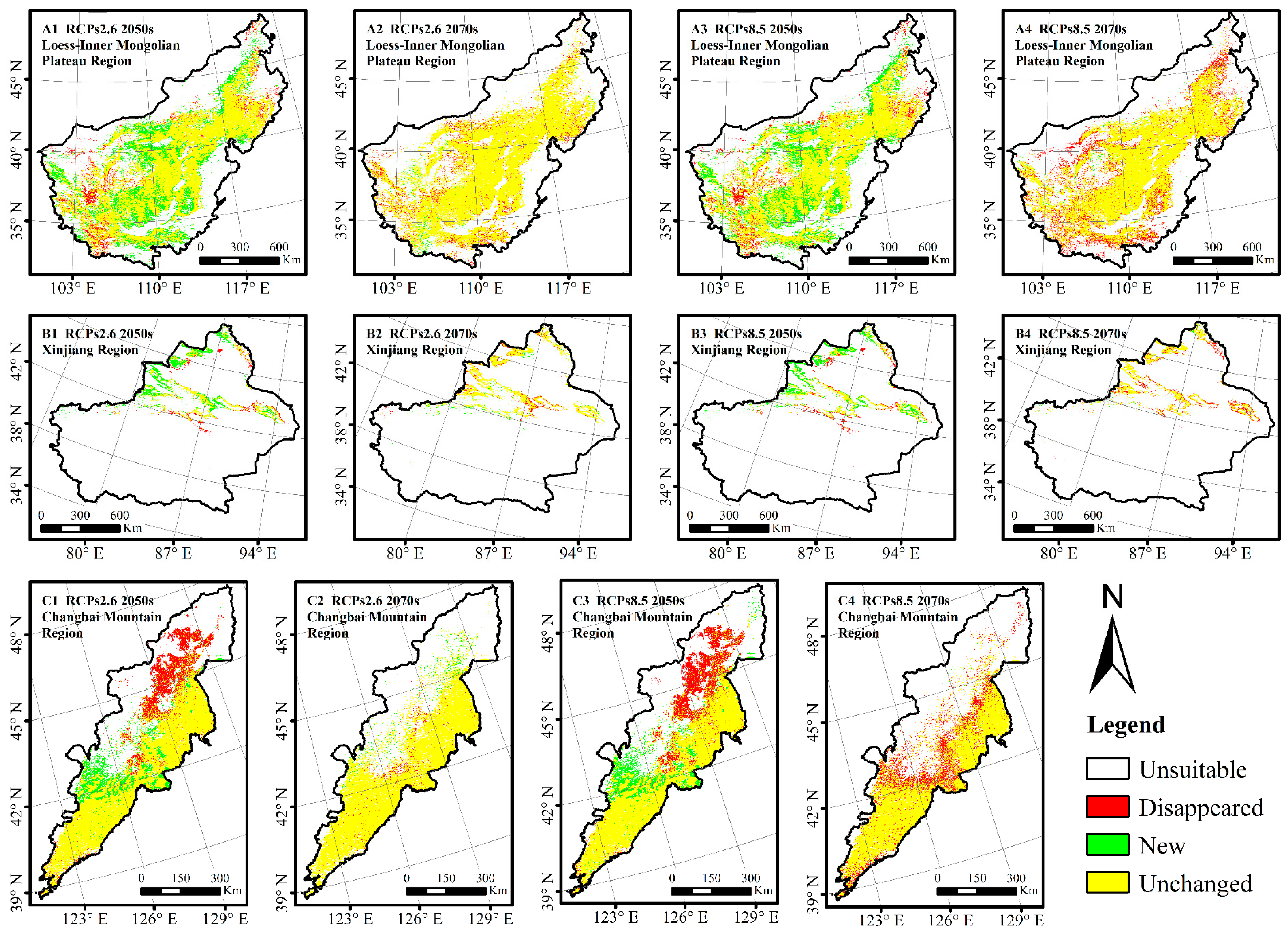
3.3. Diversified Changes of Suitable Habitat Areas among Different Regions under Future Climate

Under the future climate scenario, the variation trends of the suitable habitat area and the pattern of increase–decrease were not exactly the same among the three regions. However, by the period of the 2070s, the area of the newly increased and disappeared suitable habitat in the three regions gradually decreased compared with that in the previous period.
As far as the Loess-Inner Mongolian plateau region was concerned, in the 2050s relative to the current distribution, the area of the potential habitat increased to 74.04 × 10⁴ and 72.10 × 10⁴ km2 (Table 3). The new areas were mainly distributed around the unchanged area, while the disappeared habitat is mainly in the west and northeast of the area under the two climate scenarios (Figure 3(A1,A3)). By the 2070s, the total habitat area decreased to 68.38 × 10⁴ and 58.43 × 10⁴ km2, respectively (Table 3), and the disappeared and new regions will be distributed almost randomly around the suitable regions relative to the 2050s (Figure 3(A2,A4)).
For Xinjiang region, the new habitat area was in the northwest of Xinjiang in 2050s under the two scenarios (Figure 3(B1,B3)), amounting to 4.01 × 10⁴ and 3.42 × 10⁴ km2 (Tabble 3), and the area of the ecological suitable raised 2.67 × 10⁴ km2 with the percentage of 47.16 under RCP 2.6 in 2050s relative to current distribution, 1.89 × 10⁴ km2 for RCP 8.5. The area of ecological suitable loss was 1.35 × 10⁴ and 1.53 × 10⁴ km2, respectively, projected for the south of the Tianshan mountains (Figure 3(B1,B3)). By the 2070s, the total habitat area went down to 7.90 × 10⁴ and 5.6 × 10⁴ km2, and the disappeared and new regions appeared in a sporadic pattern throughout the entire distribution area (Figure 3(B2,B4)).
For the Changbai mountain region, the areas of the total, new, and disappeared ecological habitat were 13.81 × 10⁴, 2.06 × 10⁴, and 2.89 × 10⁴ km2, respectively, in the 2050s under RCP 2.6 and 13.23 × 10⁴, 1.94 × 10⁴, and 3.52 × 10⁴ km2 for RCP 8.5 (Table 3). The northern region disappeared seriously, while the central region gained more area (Figure 3(C1,C3)). By the 2070s, the total suitable area remained down continuously to 13.23 × 10⁴ and 10.20 × 10⁴ km2 relative to the 2050s (Table 3, Figure 3(C2,C4)).

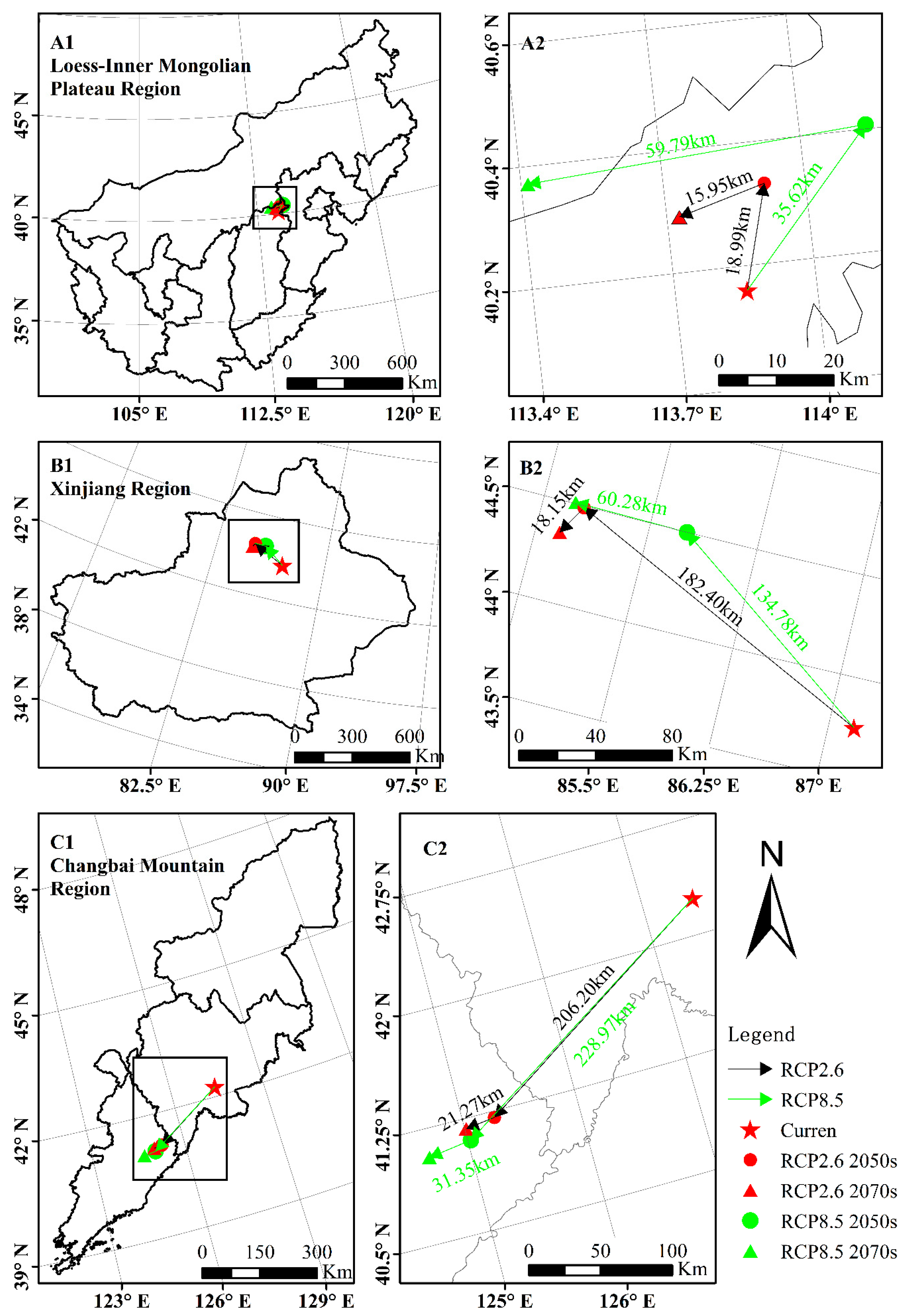
3.4. Varied Spatial Shifts of Core Distribution in China under the Future Climate Scenario

In the Loess-Inner Mongolian plateau region, the geographical centroid of the ecological habitat of Juniperus rigida Sieb. et Zucc. was located at 113.85° E and 40.16° N where the elevation was 1518 m, migrated northeastward about 18.99 km to the position of 113.91° E and 40.33° N in the 2050s, and then shifted southwestward about 15.95 km to 113.73° E and 40.29° N in the 2070s under the RCP 2.6 scenario. There were the same pattern under RCP 8.5 to RCP 2.6. The centroid moved northeastward about 35.62 km and went southwestward 59.79 km. The altitude of the geographical centroid for core distribution decreased and then increased, from 1518 m down to 1373 m and then up to 1464 m under RCP 2.6, and from 1518 m fell to 1373 m and rose to 1618 m under RCP 8.5 (Table 4, Figure 4(A1,A2)).
Talk about the Xinjiang region, the geographical centroid of the core habitat of Juniperus rigida Sieb. et Zucc., moved northwestward under the two scenarios on the whole. The center started at the position of 89.17° E and 49.36° N and stopped at 85.03° E, 44.49° N for RCP 2.6, 84.91° E, 44.35° N for RCP 8.5. Similarly, the elevation of the geographical centroid for core area showed an escalating trend and then task back under the two scenarios. The initial altitude was 2138 m, and in the 2050s descended to 2004 and 2099 m, respectively, afterwards ascending to 2070 m for RCP 2.6 and 2104 m for RCP 8.5 (Table 4, Figure 4(B1,B2)).
There was a difference in the Changbai mountain region compared with the other two regions in terms of migration direction and elevation change. The geographical centroid migrated southwesterly without changing direction, and the elevation raised continuously over the future two periods under the two scenarios. It started at 127.44° E, 42.24° N and then went through 125.27° E, 41.21° N, finally ending at 125.01° E, 41.18° N under RCP 2.6 with the distance of about 227.47 km and positioned at 124.65° E, 40.06° N with about 260.32 km for RCP 8.5. The altitude ran upward from 450 to 477 and 484 respectively (Table 4, Figure 4(C1,C2)).

4. Discussion

4.1. Suitable Distribution in Current Climate Scenario

In this study, we calibrated the MaxEnt model and projected the distribution regions of J. rigida on the national scale under the current and future climate scenario base on the climate, soil, and topographical variables. Overall, the model showed a perfect performance under all the climate scenarios [34], with the AUC 0.928 ± 0.025.
According to the estimated result, the distribution regions of Juniperus rigida Sieb. et Zucc. concentrated on three regions under current and future climate scenarios, which were renamed Xinjiang region, Loess-Inner Mongolian plateau region, and Changbai Mountain region from west to east (Figure 2). The result was in general agreement with the previous occurrence recorded in nine provinces, including Heilongjiang, Jinlin, Liaoning, Inner Mongolian, Shaanxi, Shanxi, Gansu, Ningxia, and Hebei [35]. There was ca. 86.87 × 10⁴ km2 area for the projected suitable habitat of J. rigida in China, and the largest area was located in the Loess-Inner Mongolian plateau region, whose area was ca. 61.39 × 10⁴ km2 with 70.59% of the national ecological suitable area (Table 2). There was a region that we should emphasize, the Xingjiang region. Although there were only three natural occurrence records ever in this region, we projected about 5.65 × 10⁴ km2 suitable distribution in this region. In the background of global climate warming, the arid climate and less rainfall coincided with its physiological characteristics [35] and provided inhabitable conditions for sprouting and growth of J. rigida in this region [36]. Furthermore, the Changbai Mountain region was also the major distribution area, which can be verified by the previous studies on species distribution to some degree [37].

4.2. Ecological Variables Influencing the Spatial Distribution Pattern of J. rigida

The geographical spatial distribution of plants is the result of long-term interaction between plants and the environment. Nevertheless, environmental factors do not affect the geographical spatial distribution equally. There were four identified variables that played a significant role in influencing the distribution pattern among all the factors that characterized the ecological habitat of Juniperus rigida Sieb. et Zucc. by running the model. The properties of J. rigida, light-loving and drought-resistant [35], made the specific requirements for slope (Slo) and altitude (Alt) in different distribution regions. The distribution elevation was 300~600 m in the Changbai mountain region, which was the lowest distribution area, and was ca. 1100~1600 m in Yinshan mountain, 1100~1300 m for the Erdos plateau, and 2000~2500 m for Helan mountain [35]. The complex topography was responsible for the diverse climate on a regional scale, and the slope affected the light intensity, evaporation, soil nutrients, and available water content to some extent.
The two factors associated to the temperature, mean temperature of the driest quarter (MTDq) and temperature annual range (TAR), also played important roles in affecting the distribution. It is stated that temperature was the dominant factor in the progress of the vegetative growth [38], flower bud differentiation [39], and seed dormancy and germination [40]. Temperature could germinate seeds and shortened the dormancy period caused by the encased in hard seed coat and oil [41]. The optimum germination temperature for Juniperus rigida Sieb. et Zucc. seeds was 15~25 °C, and the light could inspire its germination rate [19]. Global warming was accompanied by rising precipitation [42]. The effect of precipitation on the geographic distribution should not be ignored when we focus on the effect of temperature. We projected that the precipitation of the wettest month (PWm) and annual precipitation (AP) were also important factors in terms of percent contribution and permutation importance of all variables.

4.3. Prospective Change on Distribution in the Face of Climate Warming

With global warming, it was reported that species will either migrate [43] or change their physiology [44] to resist climate change. There may be a main trend of species migrating to high latitude or high elevation [45,46]. The mean altitude of the core suitable area gradually increased in Chanbai mountain regions, first up and then down in other two regions, over time, which may be a strategy for Juniperus rigida Sieb. et Zucc. to adapt to the changing environment (Table 3). In this respect, our results were completely consistent with those of previous studies [47]. The migration paths were almost the same in the same study area under the two different climate scenarios; nevertheless, they moved in different directions in different regions (Figure 4). The trajectory of core area centroid was triangular in the Loess-Inner Mongolian Plateau Region, first northeast and then southwest, and almost linear in the Xinjiang Region and Changbai Mountain region, northwest and southwest direction, respectively (Figurre 4). This phenomenon was mainly related to the complexity of climate change. The centroid of Changbai Mountain distribution migrated to low latitude that was different from the previous work [45,46]. The impact of global climate change on China was more obvious than other countries, and the temperature in Northeast of China rose faster than that in other regions [48]. All of those could clarify why the distribution centroid in Changbai Mountain migrated to lower latitudes rather than higher ones. In any region, the centroid shifted further under RCP 8.5 to RCP 2.6 scenario. RCP 8.5, a very high GHG emission scenario, led to robust global surface warming [22,23,24,25], affecting more prominently the distribution of J. rigida in China to RCP 2.6.
In addition to the migration of suitable areas, climate change also affected the area of suitable distribution. On the side, it is also affected the adaptability of species to climate change [49]. We gained the similar achievement of previous studies that showed that the suitable habitat range will increase as global warming intensity proceeds under the low concentration emissions pathway (RCP 2.6) [50], but excessive temperature raised might restrict plants’ diffusion under the powerful GHG emissions pathway (RCP 8.5) [51]. The suitable area increased and then decreased in the Xinjiang region and the Loess-Inner Mongolian plateau region and decreased continuously in Chanbai Mountain region in both scenarios. This may be caused by the more significant effect of climate warming and precipitation in the northeast of China than other regions [48,52]. Comparing the effects of climate change and precipitation on China [53], the change in temperature and precipitation were marked in the following areas where the area of disappeared suitable habitat were severe, including the north part of Chanbai Mountain and the south part of Taihang Mountain and Lvliang Mountain. On the contrary, the adjacent regions of Hebei, Inner Mongolia, and Shaanxi province were flooded with new distributions in the 2050s and 2070s, in which there were mild changea in temperature and precipitation under the stringent concentration emissions pathway (RCP 2.6) and the high greenhouse emission scenario (RCP 8.5) [48].

5. Conclusions

There, we projected the current and future distribution areas of Juniperus rigida Sieb. et Zucc. in China using the MaxEnt model under the climatic scenario of RCP 2.6 and RCP 8.5 for two periods, the 2050s and 2070s. These results indicated that the temperature-dependent variables affected the suitable habitat more than the factors associated with the precipitation. The suitable area increased first and then decreased on the whole, and the centroid of the core habitat migrated to high elevation. These insights were remarkable in the Changbai Mountain region under the same scenario and were more obvious under RCP 8.5 in any region. Though we gained meaningful results that will provide a more effective and evidence-based conservation strategy, they were not comprehensive, and other factors should be taken into account too, for instance, adaptability to climate change, diffusivity, and so on. However, these were unfamiliar to us in this paper.

Author Contributions

Conceptualization, D.L. and Z.L.; methodology, Z.L.; software, Z.L.; validation, D.L. and Z.L.; formal analysis, Z.L.; investigation, D.L. and Z.L.; resources, Z.L.; data curation, Z.L.; writing—original draft preparation, Z.L.; writing—review and editing, D.L.; visualization, Z.L.; supervision, D.L.; project administration, D.L.; funding acquisition, D.L. Both authors have read and agreed to the published version of the manuscript.

Funding

This work was supported by the program from the National Natural Science Foundation of China (No. 31570655).

Data Availability Statement

The bioclimatic variables are available from the WorldClim-Global Climate Database (http://worldclim.org/ (accessed on 16 July 2021)). The occurrence records of Juniperus rigida Sieb. et Zucc presented in this study are available on request from the corresponding author.

Conflicts of Interest

The authors declare no conflict of interest.

References

  1. Şahin, Ü.A.; Onat, B.; Ayvaz, C. Climate Change and Greenhouse Gases in Turkey. In Recycling and Reuse Approaches for Better Sustainability; Balkaya, N., Guneysu, S., Eds.; Environmental Science and Engineering; Springer: Cham, Switzerland, 2019; pp. 201–214. [Google Scholar]
  2. Pachauri, K.; Meyer, A. Climate Change 2014. Synthesis Report. Environ. Policy Collect. 2014, 27, 408. [Google Scholar] [CrossRef]
  3. Moraitis, M.L.; Valavanis, V.D.; Karakassis, I. Modelling the effects of climate change on the distribution of benthic indicator species in the Eastern Mediterranean Sea. Sci. Total Environ. 2019, 667, 16–24. [Google Scholar] [CrossRef]
  4. Wilson, K.L.; Skinner, M.A.; Lotze, H.K. Projected 21st-century distribution of canopy-forming seaweeds in the Northwest Atlantic with climate change. Divers. Distrib. 2019, 25, 582–602. [Google Scholar] [CrossRef] [Green Version]
  5. Nogué, S.; Rull, V.; Vegas-Vilarrúbia, T. Modeling biodiversity loss by global warming on pantepui, northern South America: Projected upward migration and potential habitat loss. Clim. Chang. 2009, 94, 77–85. [Google Scholar] [CrossRef]
  6. Yi, Y.J.; Zhou, Y.; Cai, Y.P.; Yang, W.; Li, Z.W.; Zhao, X. The influence of climate change on an endangered riparian plant species: The root of riparian Homonoia. Ecol. Indic. 2018, 92, 40–50. [Google Scholar] [CrossRef]
  7. Pinedo-Alvarez, C.; Renteria-Villalobos, M.; Aguilar-Soto, V.; Vega-Mares, J.H.; Melgoza-Castillo, A. Distribution dynamics of Picea chihuahuana Martínez populations under different climate change scenarios in Mexico. Glob. Ecol. Conserv. 2019, 17, e00559. [Google Scholar] [CrossRef]
  8. Grinnell, J. The niche-relationships of the California Thrasher. Auk 1917, 34, 427–433. [Google Scholar] [CrossRef]
  9. Elton, C.S. Animal Ecology; University of Chicago Press: Chicago, IL, USA, 1927. [Google Scholar]
  10. Hutchinson, G.E. Concluding remarks. Cold Spring Harb. Sym. 1957, 22, 415–427. [Google Scholar] [CrossRef]
  11. Busby, J.R. BIOCLIM: A bioclimate analysis and prediction system. Plant Prot. Q. 1991, 6, 8–9. [Google Scholar]
  12. Carpenter, G.; Gillison, A.N.; Winter, J. DOMAIN: A flexible modelling procedure for mapping potential distributions of plants and animals. Biodivers. Conserv. 1993, 2, 667–680. [Google Scholar] [CrossRef]
  13. Stockwell, D.; Peters, D. The GARP modelling system: Problems and solutions to automated spatial prediction. Int. J. Geogr. Inf. Sci. 1999, 13, 143–158. [Google Scholar] [CrossRef]
  14. Phillips, S.B.; Aneja, V.P.; Kang, D.; Arya, S.P. Modelling and analysis of the atmospheric nitrogen deposition in North Carolina. Int. J. Glob. Environ. Issues 2006, 6, 231–252. [Google Scholar] [CrossRef] [Green Version]
  15. Pearson, R.G.; Raxworthy, C.J.; Nakamura, M.; Peterson, A.T. Predicting species distributions from small numbers of occurrence records: A test case using cryptic geckos in Madagascar. J. Biogeogr. 2007, 1, 102–117. [Google Scholar] [CrossRef]
  16. Elith, J.; Graham, C.H.; Anderson, R.P.; Dudik, M.; Ferrier, S.; Guisan, A.; Hijmans, R.J.; Huettmann, F.; Leathwick, J.R.; Lehmann, A.; et al. Novel methods improve prediction of species’ distributions from occurrence data. Ecography 2006, 29, 129–151. [Google Scholar] [CrossRef] [Green Version]
  17. Tsoar, A.; Allouche, O.; Steinitz, O.; Rotem, D.; Kadmon, R. A comparative evaluation of presence-only methods for modelling species distribution. Divers. Distrib. 2007, 13, 397–405. [Google Scholar] [CrossRef]
  18. Qin, H.N.; Yang, Y.; Dong, S.Y.; He, Q.; Jia, Y.; Zhao, L.N.; Yu, S.X.; Liu, B.; Yan, Y.H.; Xiang, J.Y.; et al. Threatened Species List of China’s Higher Plants. Biodivers. Sci. 2017, 25, 696–744. [Google Scholar] [CrossRef] [Green Version]
  19. Liu, Y.H.; Ma, Z.H. Influencing factors on seed germination of Juniperus rigida from Helan Mountain. J. Northwest A F Univ. 2016, 44, 62–70. [Google Scholar]
  20. Gelviz-Gelvez, S.M.; Pavón, N.P.; Illoldi-Rangel, P.; Ballesteros-Barrera, C. Ecological niche modeling under climate change to select shrubs for ecological restoration in Central Mexico. Ecol. Eng. 2015, 74, 302–309. [Google Scholar] [CrossRef]
  21. Molloy, S.W.; Davis, R.A.; Van Etten, E.J. Species distribution modelling using bioclimatic variables to determine the impacts of a changing climate on the western ringtail possum (Pseudocheirus occidentals; Pseudocheiridae). Environ. Conserv. 2014, 41, 176–186. [Google Scholar] [CrossRef]
  22. Pachauri, R.K.; Allen, M.R.; Barros, V.R.; Broome, J.; Cramer, W.; Christ, R.; Church, J.A.; Clarke, L.; Dahe, Q.; Dasgupta, P.; et al. Climate Change 2014: Synthesis Report; Contribution of Working Groups I, II and III to the Fifth Assessment Report of the Intergovernmental Panel on Climate Change; Pachauri, R., Meyer, L., Eds.; IPCC: Geneva, Switzerland, 2014; p. 151. Available online: http://hdl.handle.net/10013/epic.45156.d001 (accessed on 13 April 2015).
  23. Vuuren, D.P.V.; Johannes, F.; Lamarque, J.F.; Riahi, K.; Rose, S.; Smith, S.; Hibbard, K. Work Plan for Data Exchange between the Integrated Assessment and Climate Modeling Community in Support of Phase-0 of Scenario Analysis for Climate Change Assessment (Representative Community Pathways); IPCC: Geneva, Switzerland, 2008; Available online: http://www.aimes.ucar.edu/docs/RCPhandshake.pdf (accessed on 6 October 2008).
  24. Weyant, J.; Azar, C.; Kainuma, M.; Kejun, J.; Nakicenovic, N.; Shukla, P.R.; Rovere, E.L.; Yohe, G. Report of 2.6 Versus 2.9 watts/m2 RCPP Evaluation Panel; IPCC: Geneva, Switzerland, 2009; p. 82. Available online: http://www.ipcc.ch/meetings/session30/inf6.pdf (accessed on 31 March 2009).
  25. Masson-Delmotte, V.; Zhai, P.; Pörtner, H.O.; Roberts, D.; Skea, J.; Shukla, P.R.; Pirani, A.; Moufouma-Okia, W.; Péan, C.; Pidcock, R.; et al. Summary for Policymakers. In Global Warming of 1.5 °C; An IPCC Special Report on the Impacts of Global Warming of 1.5 °C above Pre-Industrial Levels and Related Global Greenhouse Gas Emission Pathways, in the Context of Strengthening the Global Response to the Threat of Climate Change, Sustainable Development, and Efforts to Eradicate Poverty; World Meteorological Organization: Geneva, Switzerland, 2018; Available online: https://www.researchgate.net/publication/329866816_Summary_for_Policymakers_In_Global_warming_of_15C_An_IPCC_Special_Report (accessed on 1 October 2018).
  26. Wang, M.H.; Li, H.L.; Sun, X.T. Quantitative evaluation on the inter-annual and inter-decadal precipitation variability simulated by sixCMIP5 models of china. Meteorol. Mon. 2018, 44, 634–644. [Google Scholar] [CrossRef]
  27. Zhang, L.; Ding, Y.H.; Wu, T.W.; Xin, X.G.; Zhang, Y.W.; Xu, Y. The 21st century annual mean surface air temperature change and the 2 °C warming threshold over the globe and China as projected by the CMIPS models. Acta Meteorol. Sin. 2013, 71, 1047–1060. [Google Scholar] [CrossRef]
  28. Morales, N.S.; Fernández, I.C.; Baca-González, V. MaxEnt’s parameter configuration and small samples: Are we paying attention to recommendations? A systematic review. PeerJ 2017, 5, e3093. [Google Scholar] [CrossRef]
  29. Phillips, S.J.; Dudik, M. Modeling of species distributions with Maxent: New extensions and a comprehensive evaluation. Ecography 2008, 31, 161–175. [Google Scholar] [CrossRef]
  30. Rong, Z.; Zhao, C.; Liu, J.; Gao, Y.; Zang, F.; Guo, Z.; Mao, Y.; Wang, L. Modeling the Effect of Climate Change on the Potential Distribution of Qinghai Spruce (Picea crassifolia Kom.) in Qilian Mountains. Forests 2019, 10, 62. [Google Scholar] [CrossRef] [Green Version]
  31. Bewick, V.; Cheek, L.; Ball, J. Statistics review 13: Receiver operating characteristic curves. Crit. Care 2004, 8, 508–512. [Google Scholar] [CrossRef] [PubMed] [Green Version]
  32. Davies, T.J.; Purvis, A.; Gittleman, J.L. Quaternary climate change and the geographic ranges of mammals. Am. Nat. 2009, 174, 297–307. [Google Scholar] [CrossRef] [PubMed]
  33. Phillips, S.J.; A Brief Tutorial on Maxent. Exercise, American Museum of Natural History, New York. 2017. Available online: http://ncep.amnh.org/linc/linc_download.php?component_id=39 (accessed on 16 July 2021).
  34. Janitza, S.; Strobl, C.; Boulesteix, A.L. An AUC-based permutation variable importance measure for random forests. BMC Bioinf. 2013, 14, 119. [Google Scholar] [CrossRef] [Green Version]
  35. Flora of China Editorial Committee. Flora of China; Science Press and Missouri Botanical Garden Press: Beijing, China, 2006; Volume 4, p. 1999. [Google Scholar]
  36. Li, T.B.; Zhang, Y.F.; Li, D.W.; Wang, C.Y. Seed germination performance of Juniperus rigida in different regions of the Loess Plateau and its relation with ecological factors. Agric. Res. Arid. Areas 2015, 3, 139–143. [Google Scholar] [CrossRef]
  37. China forest Editorial Committee. China Forest; China Forestry Press: Beijing, China, 2000. [Google Scholar]
  38. Li, K.; Zheng, B.Q.; Wang, Y.B.; BU, W.S. Numeric dynamics of natural populations of Paeonia delavayi (Paeoniaceae). Chin. J. Plant Ecol. 2012, 36, 522–529. [Google Scholar] [CrossRef]
  39. Philip, M.P.M. Physiological Studies on Floral Bud Development and Flowering Mechanism in Tree Peony (Doctoral dissertation); Beijing Forestry University: Beijing, China, 2011. [Google Scholar]
  40. Baskin, C.C.; Baskin, J.M. Seeds: Ecology Biogeography and Evolution of Dormancy and Germination, 2nd ed.; Academic Press: San Diego, CA, USA, 2014. [Google Scholar]
  41. Li, X.Y.; He, L. Preliminary study of techniques for growing seedlings of Juniperus rigida. For. Shaanxi 2011, 3, 36. [Google Scholar]
  42. Root, T.L.; Price, J.T.; Hall, K.R.; Schneider, S.H.; Rosenzweig, C.; Pounds, J.A. Fingerprints of global warming on wild animals and plants. Nature 2003, 421, 57–60. [Google Scholar] [CrossRef] [PubMed]
  43. Hoffmann, A.A.; Sgro, C.M. Climate change and evolutionary adaptation. Nature 2011, 470, 479–485. [Google Scholar] [CrossRef]
  44. Hu, X.G.; Jin, Y.; Wang, X.R.; Mao, J.F.; Li, Y. Predicting impacts of future climate change on the distribution of the widespread conifer Platycladus orientalis. PLoS ONE 2015, 10, e0132326. [Google Scholar] [CrossRef] [PubMed]
  45. Lenoir, J.; Gégout, J.C.; Marquet, P.A.; Ruffray, P.; Brosse, H. A significant upward shift in plant species optimum elevation during the 20th century. Science 2008, 320, 1768–1771. [Google Scholar] [CrossRef] [PubMed]
  46. Bertrand, R.; Lenoir, J.; Piedallu, C.; Riofrío-Dillon, G.; De Ruffray, P.; Vidal, C.; Pierrat, J.; Gégout, J. Changes in plant community composition lag behind climate warming in lowland forests. Nature 2011, 479, 517–520. [Google Scholar] [CrossRef]
  47. Grabherr, G.; Gottfried, M.; Pauli, H. Climate effects on mountain plants. Nature 1994, 369, 448. [Google Scholar] [CrossRef]
  48. Zhou, M.Z.; Zhou, G.S.; Lv, X.M.; Zhou, L.; Ji, Y.H. Projection of temperature and precipitation changes over China under global warming of 1.5 and 2 °C. Acta Meteorol. Sin. 2019, 77, 728–744. [Google Scholar] [CrossRef]
  49. Woodward, F.I.; Williams, B.G. Climate and plant distribution at global and local scales. In Theory and Models in Vegetation Science; Prentice, I.C., van der Maarel, E., Eds.; Advances in vegetation science; Springer: Dordrecht, The Netherlands, 1987; Volume 8. [Google Scholar] [CrossRef]
  50. Ma, B.; Sun, J. Predicting the distribution of Stipa purpurea across the Tibetan Plateau via the MaxEnt model. BMC Ecol. 2018, 18, 10. [Google Scholar] [CrossRef] [Green Version]
  51. Xu, M.H.; Xue, X. Analysis on the effects of climate warming on growth and phenology of alpine plants. J. Arid Land Resour. Environ. 2013, 27, 137–141. [Google Scholar] [CrossRef]
  52. Jiang, D.B.; Fu, Y.H. Climate change over China with a 2 °C global warming. Chin. J. Atmos. Sci. 2012, 36, 234–246. [Google Scholar] [CrossRef]
  53. Su, Q.H.; Zhou, R.J.; Ke, Z.J.; Liu, C.Z.; Du, L.M.; Yan, Y. Optimal weighted model for ensemble forecast of the surface air temperature in mainland China and its regional applications. J. Univ. Sci. Technol. China 2017, 48, 199–209. [Google Scholar] [CrossRef]
Figure 1. Distribution records of J. rigida in China.
Forests 12 01140 g001
Figure 2. Potential distribution area of Juniperus rigida Sieb. et Zucc. under the current climate. The potential distribution of China was illustrated in (A), and (B), (C) and (D) shown the distribution of the Loess-Inner Mongolian plateau region, Xinjiang region and Changbai Mountain region, respectively.
Forests 12 01140 g002
Figure 3. The potential distribution range shift in the extent of Juniperus rigida Sieb. et Zucc. under the low concentration emissions pathway (RCP2.6) in three regions. The changes in the 2050s to current showed in (A1), (B1), and (C1) under RCP2.6, and in (A3), (B3), and (C3) under RCP 8.5. (A2), (B2), and (C2) illustrated the changes in 2070s relative to 2050s under RCP 2.6, (A4), (B4), and (C4) for RCP 8.5.
Forests 12 01140 g003
Figure 4. The core distributional shift under future climate scenarios for Juniperus rigida Sieb. et Zucc. in three main distribution areas. (A1) illustrated the shift path in the Loess-Inner Mongolian region—full figure, (A2) illustrated the shift path in the Loess-Inner Mongolian region—detail figure, (B1) for the Xinjiang region—full figure, (B2) for the Xinjiang region—detail figure, (C1) for the Changbai Mountain region—full figure, (C2) for the Changbai Mountain region—detail figure.
Forests 12 01140 g004
Table 1. Percentage contributions and permutation importance of the environmental variables.
AbbreviationVariables DescriptionPercent Contribution (%)Permutation Importance
SloSlope16.87637.3039
AltAltitude15.785129.669
MTDqMean Temperature of Driest Quarter12.83161.4061
TARTemperature Annual Range11.677311.4124
PWmPrecipitation of Wettest Month6.62540.7003
SpHSubsoil pH5.39581.2187
PSPrecipitation Seasonality4.95893.4087
RHRelative Humidity3.92512.8779
TSTemperature Seasonality3.86795.0902
IsoIsothermality3.81069.43
InsInsolation Hour3.30073.063
AspAspect2.10472.1337
TpHTopsoil pH1.95481.8882
MDRMean Diurnal Range1.88513.2606
AMTAnnual Mean Temperature1.40838.0216
TTEXTopsoil Texture1.20190.9042
AWCAvailable Water Content1.1130.9102
APAnnual Precipitation0.64864.1459
PCqPrecipitation of Coldest Quarter0.28261.3119
SOCSubsoil organic content0.18340.6614
MTWmMax Temperature of Warmest Month0.15261.1502
TECETopsoil Electric Conductivity0.01050.0318
Table 2. Summary of the area and proportion of various suitable distribution areas of J. rigida in China and three regions.
RegionsGeneral DistributionModerate DistributionCore DistributionTotal
Area
(104 km2)
Percentage
(%)
Area
(104 km2)
Percentage
(%)
Area
(104 km2)
Percentage
(%)
Area
(104 km2)
China49.5957.0827.1531.2510.1311.6686.87
Changbai Mountain region6.5344.586.3243.121.8012.2914.65
Loess-Inner Mongolian
Plateau Region
34.9556.9318.4330.028.0113.0461.39
Xinjiang Region4.0671.821.3919.250.203.895.65
Table 3. Area variation of the suitable habitat in the three kind regions under the future climate scenarios relative to current.
ScenarioTypeXinjiang Region
(104 km2)
Loess-Inner Mongolian
Platea Region (104 km2)
Changbai Mountain
Region (104 km2)
2050s2070s2050s2070s2050s2070s
CurrentTotal5.65161.39414.646
RCP 2.6Disappeared−1.348−1.329−5.789−7.253−2.887−2.891
New4.0123.58018.43414.2372.0572.055
Unchanged4.3034.32255.60454.14011.75611.753
Total8.3167.90274.03968.37713.81313.808
RCP 8.5Disappeared−1.525−2.415−6.094−12.693−3.352−5.244
New3.4162.36216.7999.7291.9430.806
Unchanged4.1263.23655.30048.70111.2849.392
Total7.5425.59872.09958.43013.22710.198
Table 4. The geographic coordinates of the core areas and the average elevation of the suitable regions. The distances represented the migration distance relative to the previous time point. The altitude means the average elevation of the core areas.
RegionsScenariosPeriodsLongitudeLatitudeAltitude (m)Distance (km)
Changbai Mountain
region
Current127.44° E42.24° N450——
RCP 2.62050s125.27° E41.21° N470206.2
2070s125.01° E41.18° N47721.27
RCP 8.52050s125.03° E41.10° N465228.97
2070s124.65° E41.06° N48431.35
Loess-Inner Mongolian
Plateau Region
Current113.85° E40.16° N1518——
RCP 2.62050s113.91° E40.33° N137318.99
2070s113.73° E40.29° N146415.95
RCP 8.52050s114.14° E40.41° N137335.62
2070s113.41° E40.37° N161859.79
Xinjiang RegionCurrent87.17° E43.76° N2138——
RCP 2.62050s85.03 ° E44.49° N2004182.4
2070s84.91° E44.35° N207018.15
RCP 8.52050s85.76° E44.50° N2099134.78
2070s84.97° E44.51° N210460.28
Publisher’s Note: MDPI stays neutral with regard to jurisdictional claims in published maps and institutional affiliations.

