Prediction Comparison of Stand Parameters and Two Ecosystem Services through New Growth and Yield Model System for Mixed Nothofagus Forests in Southern Chile

Abstract

Forest managers need tools to predict the behavior of forests not only for the main stand parameters, such as basal area and volume, but also for ecosystem services such as timber volume and carbon sequestration. Useful tools to predict these parameters are growth and yield model systems with several possible options for modeling, such as the whole stand-level model, with or without diameter distribution generation, individual tree-level model, and compatibility models. However, those tools are scarce or developed mainly for forest plantations that are mostly located in the northern hemisphere. Thus, this study focuses on analyzing predictions of several growth and yield models built for native mixed Nothofagus forests from southern Chile, using the simulator Nothopack. A dataset of 19 permanent plots with three measurements were used for comparing the different models. Individual tree-level simulation presented the best goodness-of-fit statistics for stand parameters and ecosystem services. For example, the basal area gave an R²_emp of 0.97 and 0.87 at 6 and 12 years of projection. However, the stand-level simulations with a generation of diameter distribution and both compatibility models showed satisfactory performance, both in accuracy and bias control. The simulator Nothopack, which has the capability of obtaining detailed outputs, is a useful tool to support management plans for these forest ecosystems.

1. Introduction

Growth and yield (G&Y) models help to represent the dynamics of natural and artificial forest stands and they include growth, mortality, and other modules to describe changes in stand structure [1]. Forest G&Y models can be classified into stand-level (low resolution) or individual-level (high resolution) models [2]. Stand-level models are those in which the modeling units are aggregated parameters such as basal area, stocking, and site productivity [3]. In contrast, individual-level models keep track and describe each tree in the stand. Both levels have advantages and disadvantages: stand-level models present well-behaved predictions in the long-term for stand parameters; however, they are inadequate to predict tree variables (such as diameter distributions or individual competition). In contrast, individual-level models are better at predicting the variables of trees and hence key information concerning timber assortments, while often lacking precision when summarizing to stand-level parameters [4].

To exploit the advantages of both model types and to improve predictions, mathematical methods have been developed to link stand- and individual-level models into a compatible system [5,6,7,8]. For instance, predicted individual tree basal areas can be adjusted so that their sum equals a predicted stand-level total basal area [4]; thus, making these predictions compatible. Likewise, the predicted individual mortality probabilities from an individual-level simulation can be adjusted to match the predicted total number of trees from a stand-level model [9]. As these adjustments keep individual tree information, they are expected to be more accurate, particularly for volume and diameter distribution predictions.

The G&Y models for natural stands are complex given the presence of a combination of several species and cohorts that often have different growth and mortality dynamics, in addition to the added complexity of modelling competition at all levels. For this reason, these natural stands often need to be modelled at individual or cohort level in order to consider all these dynamics. However, data are often limited and there are few G&Y models that have been developed that consider individual or cohort level data [10]. Mixed natural forest G&Y models could greatly benefit from compatibility methods and improved predictability.

A temperate natural forest that requires a G&Y model is the Nothofagus forest in southern Chile, known as RORACO, for the dominance of the emergent trees of Raulí (N. alpina (Poepp. & Endl.) Oerst.), Roble (N. obliqua (Mirb.) Oerst.), and Coigüe (N. dombeyi (Mirb.) Oerst.). The simulator Nothopack was built for those forests, specifically for second-growth stands, incorporating a stand-level basal area growth model [11], a tree individual-level diameter growth model [12], and two compatibility approaches. This is the first simulator system for the complete distribution area of this native second-growth forest that covers more than 1.4 million hectares (10.8% of total native forest of Chile; [13]).

Our society favors the sustainable use of natural resources such as native forests, but not only as a source of market-products but also as a generator of ecosystem services [14]. Therefore, analytical tools, such as G&Y models, must be capable of incorporating products (e.g., saw-log) together with other ecosystem services (e.g., carbon sequestration) in their evaluations. Typically, this information is scarce or available with considerable errors, and this is even more pronounced for native forests in most developing countries. In particular, for RORACO forests, there are very few publications with information related to the carbon sequestration of above-ground tree dry matter biomass [15].

The main objective of this study is to evaluate different G&Y strategies for RORACO forests in southern Chile. The specific objectives are (1) to validate predictions of stand-level, individual-level, and two compatibility simulations against independent data (not used for model fitting); and (2) to generate predictions of two ecosystem services, including fiber provision and carbon sequestration, as a regulation service for these forests.

2. Materials and Methods

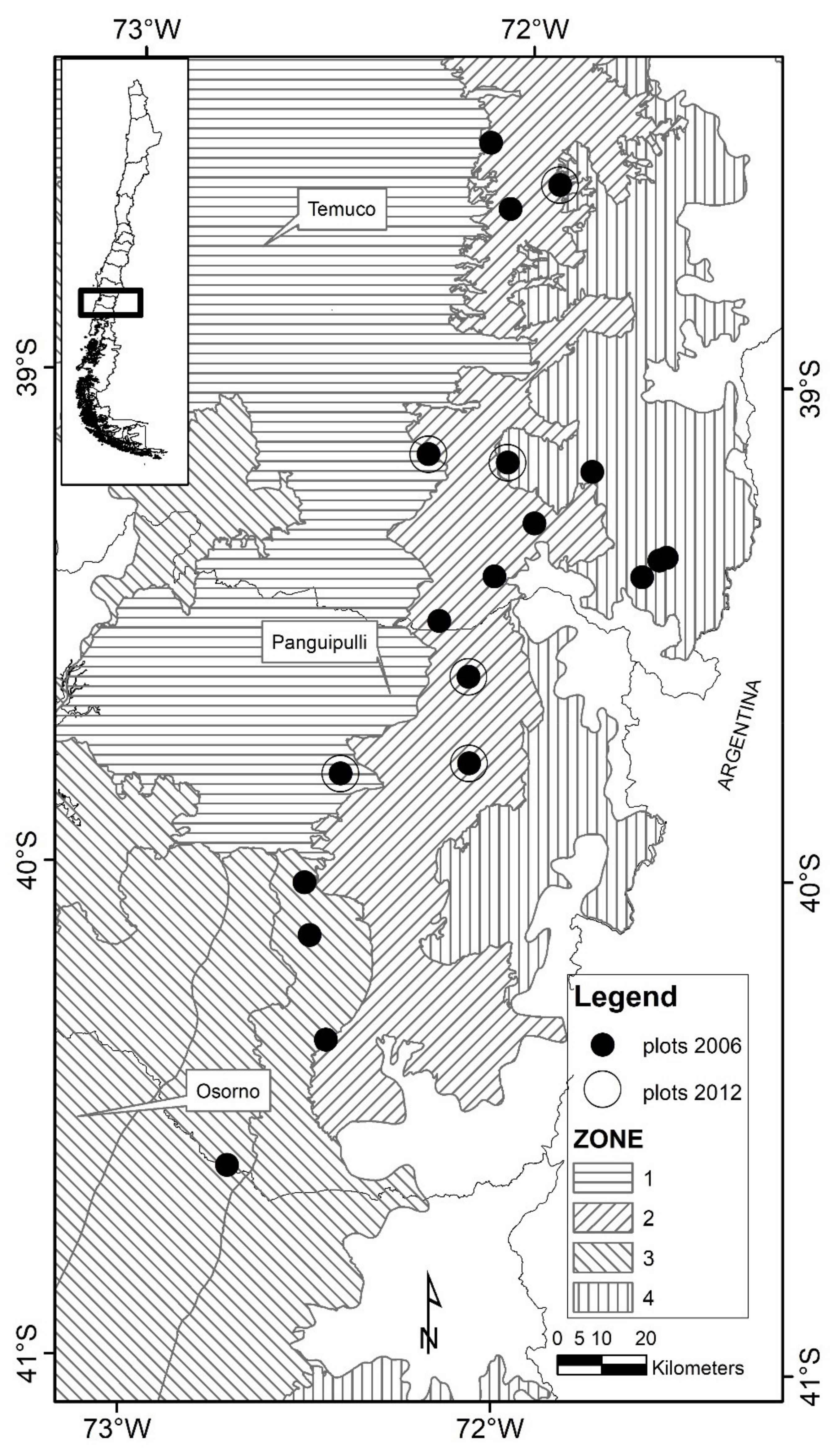
2.1. Data Description

Data for this study originated from 19 permanent plots (PP) established in second-growth RORACO forests in southern Chile, dominated mainly by N. obliqua and located between the 38°30′ and 42°40′ S latitude (Figure 1). The research project D97I1065 from the Universidad Austral de Chile established the PP network in 2000, with areas of 250 or 500 m² (<4800 trees ha⁻¹) depending on the stand density. These plots have the following two remeasurements: all plots in 2006, and a subset of six plots in 2012.

Trees above 5 cm in diameter at breast height (DBH) and taller than 2 m were measured for DBH (cm). Total height (H, m) was sampled sequentially for a subset of 15 trees per plot. Nothofagus species were identified (SP, with N. alpina (1); N. obliqua (2); and N. dombeyi (3)), and the rest were recorded as other species (4). Sociological status (SS), according to vertical stratification was also obtained (dominant (1); codominant (2); intermediate (3); and suppressed (4)). Increment cores, at breast height, were extracted from the same subset of trees for total height to determine breast height age (years) at the first measurement.

Several stand-level variables were calculated or estimated using tree-level information. Total basal area (BA, m² ha⁻¹), total number of trees (NHA, trees ha⁻¹), quadratic diameter (QD, cm), basal area of Nothofagus species (BAN, m² ha⁻¹), the number of Nothofagus trees (NHAN, trees ha⁻¹), and the proportion of basal area and number of Nothofagus trees (PBAN, PNHAN) were all calculated for each plot-measurement. In addition, dominant age at breast height (AGE, years) and dominant height (HD, m) were obtained with the average of the thickest 100 trees per hectare. Site index (SI) was estimated using dominant height-site models previously reported by Moreno et al. [16]. All plots were assigned a growth zone (ZONE 1, 2, 3, and 4), according to Moreno et al. [16] (see Figure 1). Stand Density Index (SDI, trees ha⁻¹) was calculated using the following expression: SDI = NHA × (25.4/QD)^β [17], where β = −1.4112 (as reported by Gezan et al. [18]) (

Table 1. Stand parameters in the permanent plots in second-growth RORACO forests in southern Chile established in 2000 and remeasured in 2006 and 2012.

	2000 (n = 19)		2006 (n = 19)		2012 (n = 6)
Variable	Mean (sd)	Range	Mean (sd)	Range	Mean (sd)	Range
AGE	40.8 (8.7)	20.7–52.3	47.4 (8.8)	26.7–59.3	51.4 (10.2)	32.7–61.4
HD	27.4 (6.0)	17.6–41.9	29.4 (5.4)	21.3–39.5	33.3 (5.7)	24.6–41.4
SI	15.3 (3.6)	8.7–23.8	14.7 (3.5)	8.2–21.7	17.3 (3.0)	14.7–23.0
BA	43.4 (11.0)	23.5–71.5	46.7 (11.1)	27.8–74.8	49.0 (9.6)	33.2–62.7
NHA	1900.0 (1103.0)	580.0–4160.0	1692.0 (899.0)	460.0–3560.0	1563.0 (789.0)	860.0–3080.0
QD	19.1 (6.0)	8.5–32.4	20.6 (6.0)	10.0–34.5	21.3 (5.2)	11.7–26.4
BAN	36.6 (10.3)	15.6–57.8	39.0 (9.9)	22.2–60.2	44.1 (10.3)	31.7–61.6
NHAN	1256.0 (793.0)	400.0–3400.0	1,046.0 (648.0)	380.0–3080.0	1118.0 (858.0)	460.0–2760.0
PNHAN	0.7 (0.2)	0.2–1.0	0.7 (0.2)	0.2–1.0	0.7 (0.2)	0.4–0.9
PBAN	0.9 (0.2)	0.4–1.0	0.8 (0.2)	0.5–1.0	0.9 (0.1)	0.7–1.0
SDI	1039.0 (251.0)	642.0–1674.0	1,066.0 (248.0)	599.0–1660.0	1079.0 (129.0)	908.0–1284.0

Note. AGE: dominant age (years), HD: dominant height (m), SI: site index (m), BA: total basal area (m² ha⁻¹), NHA: total number of trees (trees ha⁻¹), QD: mean quadratic diameter (cm), BAN: basal area of Nothofagus (m² ha⁻¹), NHAN: number of Nothofagus trees (trees ha⁻¹), PNHAN: proportion number of Nothofagus trees (0–1), PBAN: proportion of BA of Nothofagus (0–1), SDI: stand density index (trees ha⁻¹).

).

2.2. Simulations

Growth simulations were developed to compare the behavior and uncertainties in stand-parameters and the provision of ecosystem services, such as timber volume and carbon sequestration. For this study, the available simulator Nothopack [19], built for RORACO second growth forest, was used. The simulation types considered were stand-level without generation of a diameter distribution (S1), stand-level incorporating a generated diameter distribution (S2), individual-level (T), yield compatibility (YC), and growth compatibility (GC). These two compatibility simulations integrated results from S1 and T (further details of these methods are presented below). For all simulations, growth estimates and predictors were updated annually until projection age. Further details of the models associated with these simulations are presented below. The independent dataset used to assess these simulations corresponded to the remeasurements of the 19 plots from the PP network. The first projected period corresponded to six years between 2000 and 2006 and from 2006 to 2012. A second projected period for analyzing corresponded to 12 years from 2000 to 2012.

2.2.1. Stand-Level without Diameter Distribution Simulation

The Nothopack’s stand-level simulation has a growth module and a mortality module. The first performs the estimation of the basal area annual growth (BA), specifically, the sum of basal areas of N. alpina, N. obliqua, and N. dombeyi (BAN), and the basal areas of other companion species (BAC). The second module incorporates a modification from Reineke’s self-thinning models to estimate future stand density. Further details are presented in Palmas et al. [11].

The stand-level basal area growth models use predictors AGE, SI, NHA, PNHAN, and PBAN [11] in the following expressions:

$$\ln \left(\mathrm{BAN}\right)={\widehat{\beta }}_0+{\widehat{\beta }}_1\ln \left(\mathrm{AGE}\right)+{\widehat{\beta }}_2\ln \left(\mathrm{SI}\right)+{\widehat{\beta }}_3\ln \left(\mathrm{NHA}\right)+{\widehat{\beta }}_4\ln \left(\mathrm{PBAN}\right)$$

(1)

$$\ln \left(\mathrm{BAC}\right)={\widehat{\beta }}_0+{\widehat{\beta }}_1\ln \left(\mathrm{AGE}\right)+{\widehat{\beta }}_2\ln \left(\mathrm{PNHAN}\right)+{\widehat{\beta }}_3\ln \left(\mathrm{PBAN}\right)$$

(2)

where $\ln$ is the natural logarithm and parameter values are shown in the Appendix A.

The compatible projection models to predict futures values (BAN₁ and BAC₁) based on current conditions (BAN₀ and BAC₀) are as follows:

$${\mathrm{BAN}}_1={\mathrm{BAN}}_0{\left(\frac{{\mathrm{AGE}}_1}{{\mathrm{AGE}}_0}\right)}^{{\widehat{\beta }}_1}{\left(\frac{{\mathrm{NHA}}_1}{{\mathrm{NHA}}_0}\right)}^{{\widehat{\beta }}_3}{\left(\frac{{\mathrm{PBAN}}_1}{{\mathrm{PBAN}}_0}\right)}^{{\widehat{\beta }}_4}$$

(3)

$${\mathrm{BAC}}_1={\mathrm{BAC}}_0{\left(\frac{{\mathrm{AGE}}_1}{{\mathrm{AGE}}_0}\right)}^{{\widehat{\beta }}_1}{\left(\frac{{\mathrm{PNHAN}}_1}{{\mathrm{PNHAN}}_0}\right)}^{{\widehat{\beta }}_2}{\left(\frac{{\mathrm{PBAN}}_1}{{\mathrm{PBAN}}_0}\right)}^{{\widehat{\beta }}_3}$$

(4)

where the $\widehat{\beta }$ coefficients are the same parameter estimates from Equations (1) and (2).

PBAN was kept constant over the projection time (PBAN₁ = PBAN₀), and PNHAN₁ was modified over time, incorporating the difference between year 0 and 1, using the following equation for each year:

$$\mathrm{logit}\left(\mathrm{PNHAN}\right)=\ln \left(\frac{\mathrm{PNHAN}}{1-\mathrm{PNHAN}}\right)={\widehat{\beta }}_0+{\widehat{\beta }}_1\mathrm{PBAN}+{\widehat{\beta }}_2\mathrm{AGE}$$

(5)

where the $\widehat{\beta }$ coefficients also are shown in the Appendix A and other terms were explained previously.

The stand-level mortality model is an annual projection of NHA based on the expression from Reineke [20] and defined by the following two parameters: $\widehat{\alpha }$ and $\widehat{k}$. The original model was presented by Palmas et al. [11] and parameter estimates are shown in the Appendix A, and its expression is as follows:

$${\mathrm{NHA}}_1=\widehat{k}*\exp (\ln \left({\mathrm{NHA}}_0\right)\left(1-\widehat{\alpha }\mathsf{\Delta }\mathrm{t}\frac{{\mathrm{QD}}_0}{{\mathrm{QD}}_{0\max }}\right))$$

(6)

where NHA₀ is the current number of trees per hectare, $\mathsf{\Delta }\mathrm{t}$ is the number of years between growth periods, QD₀ is the current quadratic diameter, and QD_{0 max} is the current maximum quadratic diameter defined by the following:

$${\mathrm{QD}}_{0\max }=\exp \left(\frac{ln\left({\mathrm{NHA}}_0-\widehat{\alpha }\right)}{\widehat{\beta }}\right)$$

(7)

where $\widehat{\alpha }$ varies depending on if the stand is dominated by N. alpina $\left({\widehat{\alpha }}_1\right)$, N. obliqua $\left({\widehat{\alpha }}_2\right),$N. dombeyi $\left({\widehat{\alpha }}_3\right)$, or a mix of them $\left({\widehat{\alpha }}_4\right)$, and $\widehat{\beta }$ is a constant for all stands [18].

Total stand volume (VHA, m³ ha⁻¹) was estimated using the following general volume equation proposed by Gezan and Ortega [21] with BA, HD, PNHAN, and PBAN as predictors:

$$\mathrm{VHA}={\widehat{\beta }}_0\left[{\mathrm{BA}}^{{\widehat{\beta }}_1}{\mathrm{HD}}^{{\widehat{\beta }}_2}{\mathrm{PNHAN}}^{{\widehat{\beta }}_3}PBA{N}^{{\widehat{\beta }}_4}\right]$$

(8)

The parameter estimates are presented in the Appendix A.

2.2.2. Stand-Level with Diameter Distribution Simulation

This simulation used the same models for basal area growth, and mortality as in Section 2.2.1, but with the generation of the following three-parameter Weibull-based diametric distribution model:

$$f\left(x\right)=\frac{C}{B}\left[{\left(\frac{x-A}{B}\right)}^{C-1}\right]\exp \left[{\left(\frac{x-A}{B}\right)}^C\right]$$

(9)

where $f\left(x\right)$ is the probability evaluated at x, A is the position parameter (set at 5 cm), and B and C are scale and shape parameters, respectively. These were obtained using the parameter recovery method as described by Gezan and Ortega [21], and they differ among species according to the following equations.

N. alpina (1):

$$\mathrm{B}={\widehat{\beta }}_0+{\widehat{\beta }}_1{\mathrm{QD}}_1+{\widehat{\beta }}_2\mathrm{PNHAN}+\frac{{\widehat{\beta }}_3}{\mathrm{BA}}$$

(10)

$$\mathrm{C}={\widehat{\beta }}_0+{\widehat{\beta }}_1\mathrm{B}+{\widehat{\beta }}_2{\mathrm{QD}}_1$$

(11)

N. obliqua (2):

$$\mathrm{B}={\widehat{\beta }}_0+{\widehat{\beta }}_1{\mathrm{QD}}_2+{\widehat{\beta }}_2\mathrm{PNHAN}+{\widehat{\beta }}_3\ln \left(\mathrm{RS}\right)$$

(12)

$$\mathrm{C}={\widehat{\beta }}_0+{\widehat{\beta }}_1\mathrm{B}+{\widehat{\beta }}_2{\mathrm{QD}}_2+\frac{{\widehat{\beta }}_3}{\mathrm{QD}}$$

(13)

N. dombeyi (3):

$$\mathrm{B}={\widehat{\beta }}_0+{\widehat{\beta }}_1{\mathrm{QD}}_3$$

(14)

$$\mathrm{C}={\widehat{\beta }}_0+{\widehat{\beta }}_1\mathrm{B}+{\widehat{\beta }}_2{\mathrm{QD}}_3+\frac{{\widehat{\beta }}_3}{\mathrm{QD}}$$

(15)

Companion species (4):

$$\mathrm{B}={\widehat{\beta }}_0+{\widehat{\beta }}_1{\mathrm{QD}}_4+{\widehat{\beta }}_2\mathrm{NHAN}$$

(16)

$$\mathrm{C}={\widehat{\beta }}_0+{\widehat{\beta }}_1\mathrm{B}+{\widehat{\beta }}_2{\mathrm{QD}}_4$$

(17)

where sub-index for stand parameters correspond to values associated with the specific species, relative spacing was calculated using the expression RS = [(10,000/NHA)0.5]/HD * 100, and parameter estimates are shown in the Appendix A.

The above models allow the estimation of BA and NHA for each diameter class and species. Volume was later calculated per diameter class using available parametric height model (H, m) (Equation (18)) and a taper equation (Equation (19)) reported by Gezan et al. [22]. The values of BA, NHA, and volume for DBH classes were aggregated to stand-level.

The general height parametric model is shown as follows with different parameter estimates based on ZONE and dominant species (≥70% in BA):

$$\mathrm{H}={\widehat{\beta }}_0+{\widehat{\beta }}_1\mathrm{HD}+{\widehat{\beta }}_2{\mathrm{QD}}^{0.95}+{\widehat{\beta }}_3\exp \left(\propto \mathrm{DBH}\right)+{\widehat{\beta }}_4{\mathrm{HD}}^3\exp \left(\propto \mathrm{DBH}\right)+{\widehat{\beta }}_5{\mathrm{QD}}^3\exp \left(\mathsf{\alpha }\mathrm{DBH}\right)$$

(18)

where the constant $\mathsf{\alpha }=-0.08$ and the rest of the parameters are shown in the Appendix A.

The following taper model was used to obtain total tree volume and per product volume, which has different parameter estimates by species:

$$\ln \left({\mathrm{d}}_j\right)={\widehat{\beta }}_0+{\widehat{\beta }}_1\ln \left(\mathrm{DBH}\right)+{\widehat{\beta }}_{2}DBH+{\widehat{\beta }}_3\ln \left(\mathrm{x}\right)\left(z^2\right)+{\widehat{\beta }}_4\ln \left(\mathrm{x}\right)\ln \left(\mathrm{z}\right)+{\widehat{\beta }}_5\ln \left(\mathrm{x}\right)\left(z^{0.5}\right)+{\widehat{\beta }}_6\ln \left(\mathrm{x}\right)\exp \left(z\right)+{\widehat{\beta }}_7\ln \left(\mathrm{x}\right)(\frac{\mathrm{DBH}}{\mathrm{H}})$$

(19)

where z = h_j/H, x = (1 − z^0.5)/(1 − 0.2^0.5), d_j is the section diameter without bark (cm), h_j is the section height (m), and the other terms were described previously. Parameter estimates also are shown in the Appendix A.

2.2.3. Tree-Level Simulation

The individual tree simulation for Nothopack has an annual growth tree DBH module, and it uses the same stand-level mortality module as in previous simulations. Volume was calculated by each tree using the taper Equation (19) and then aggregated to stand-level. Here, in each year of the time projection, the DBH was updated by adding the following estimated annual diameter increment (AIDBH, mm year⁻¹) based on the model [12]:

$$\ln \left(\mathrm{AIDBH}\right)={\widehat{\beta }}_0+{\widehat{\beta }}_1\ln \left(\mathrm{BALn}+10\right)+{\widehat{\beta }}_2\mathrm{SDI}+{\widehat{\beta }}_3\ln \left(\mathrm{DBH}\right)+{\widehat{\beta }}_4\ln \left(\mathrm{AGE}\right)+{\widehat{\beta }}_5\mathrm{SS}$$

(20)

where BALn is the basal area of larger trees for Nothofagus (m² ha⁻¹) and other terms were described before. All coefficient values can be found in the Appendix A.

2.2.4. Compatibility Simulations

Two compatibility methods were considered to calibrate the projections of the individual-level models, referred to as proportional yield compatibility (YC) and proportional growth compatibility (GC; also known as disaggregation) [4,23]. Both first calibrate individual mortality probabilities based on the stand-level mortality projection (NHA₁, from Equation (6)), and then calibrate each tree’s DBH to equate the summation of their basal area to the stand-level BA simulation (BA₁, from Equation (3)). The expressions for the YC method are as follows:

$${\widetilde{FT}}_{1i}={\widehat{FT}}_{1i}\left(\frac{{\widehat{\mathrm{NHA}}}_1}{{{\displaystyle \sum }}_{i=1}^n{\widehat{FT}}_{1i}}\right)$$

(21)

$${\widetilde{DBH}}_{1i}^2={\widehat{DBH}}_{1i}^2\left(\frac{{\widehat{\mathrm{BA}}}_1/\mathrm{K}}{{{\displaystyle \sum }}_{i=1}^n{\widehat{FT}}_{1i}{\widehat{DBH}}_{1i}^2}\right)$$

(22)

where ${\widetilde{FT}}_{1i}$ and ${\widehat{FT}}_{1i}$ are the calibrated and predicted expansion factors (the number of trees that each sample tree represents) for $i$th tree at time 1, respectively; ${\widehat{\mathrm{NHA}}}_1$ is the trees per hectare at time 1; ${\widetilde{DBH}}_{1i}^2$ and ${\widehat{DBH}}_{1i}^2$ are the calibrated and predicted squared diameters for the $i$th tree at time 1, respectively. ${\widehat{\mathrm{BA}}}_1$ is the predicted basal area at time 1 from Equation (3); and $\mathrm{K}=\pi /\mathrm{40,000}$, is a constant.

The expressions for the GC method are as follows:

$${\widetilde{FT}}_{1i}={\widehat{FT}}_{1i}^m,\mathrm{subject}\mathrm{to}{{\displaystyle \sum }}_{i=1}^n{\widetilde{FT}}_{1i}={\widehat{\mathrm{NHA}}}_1$$

(23)

$${\widetilde{DBH}}_{1i}^2=DB{H}_{0i}^2+\left(\frac{{\widehat{BA}}_1/K-{{\displaystyle \sum }}_{i=1}^n{\widehat{FT}}_{1i}DB{H}_{0i}^2}{{{\displaystyle \sum }}_{i=1}^n{\widehat{FT}}_{1i}\left({\widehat{DBH}}_{1i}^2-DB{H}_{0i}^2\right)}\right)\left({\widehat{DBH}}_{1i}^2-DB{H}_{0i}^2\right)$$

(24)

where $DB{H}_{0i}^2$ is the squared diameter of the $i$th tree at time 0 and all other terms were previously defined. Note that Equation (23) requires a search algorithm to estimate a power value m that makes the sum of the predicted expansion factors equal to ${\widehat{\mathrm{NHA}}}_1$.

2.3. Evaluation of Ecosystem Services

The following two ecosystem services were considered based on the growth and yield simulations: provisioning and regulating services. The first is associated with the provision of fiber wood, specifically saw-log (SL), pulpwood (PW), and residual lumber (RES). The second is associated with carbon sequestration, which, in this study, aimed at total tree living biomass. Using taper models, it was possible to estimate different stem products for S2 and T simulations; however, for S1 simulation, this was not possible.

At present, the typical market log products in Chile are [24] (1) SL with a length of 3.7 m and a minimum log diameter of 24 cm, (2) PW with a length of 2.44 m and a minimum diameter of 10 cm, and (3) the remaining individual stem volume corresponding to RES. In the case of carbon sequestration, the carbon stock calculation (C, tonne C), above-ground tree dry matter biomass (AGB, tonne d.m.) was estimated based using specific models for each species previously reported by Milla et al. [25], which are as follows:

$${\mathrm{AGB}}_{N.alpina}=\frac{{\widehat{\beta }}_0+{\widehat{\beta }}_1{\mathrm{DBH}}^{{\widehat{\beta }}_2}{\mathrm{H}}^{{\widehat{\beta }}_3}}{1000}$$

(25)

$${\mathrm{AGB}}_{N.obliqua}=\frac{{\widehat{\beta }}_0+{\widehat{\beta }}_1{\mathrm{DBH}}^{{\widehat{\beta }}_2}{\mathrm{H}}^{{\widehat{\beta }}_3}}{1000}$$

(26)

$${\mathrm{AGB}}_{N.dombeyi}=\frac{\exp ({\widehat{\beta }}_0+{\widehat{\beta }}_1\ln \left(\mathrm{DBH}\right)+{\widehat{\beta }}_2\ln \left({\mathrm{DBH}}^2\mathrm{H}\right)}{1000}$$

(27)

$${\mathrm{AGB}}_{Companion}=\frac{{\widehat{\beta }}_0{\mathrm{DBH}}^{{\widehat{\beta }}_1}}{1000}$$

(28)

where model terms were already described, and parameter estimates can be found in the Appendix A.

A root–shoot ratio (R, tonne d.m.) of 0.24 was considered the same for all species using tier 1 for temperate broadleaf forests [26]. Carbon fraction (CF, tonne d.m.⁻¹) was specific to species with values of 0.4445, 0.4248, 0.4370, and 0.4282 for N. alpina, N. obliqua, N. dombeyi, and companion species, respectively [27]. The formula considered to calculate carbon stock was as follows:

$$\mathrm{C}={\displaystyle \sum }_{i=1}^4[AG{B}_i\left(1+R\right)]\times C{F}_i$$

(29)

where i = 1, 2, 3, and 4 corresponding to N. alpina, N. obliqua, N. dombeyi, and companion species, respectively. Finally, carbon sequestration over the simulation period was calculated by subtracting the carbon stock at the initial time of simulation from the carbon stock at the end of the projection.

The following goodness-of-fit measures were used to evaluate all the following simulations: empirical coefficient of correlation (R²_emp), relative root mean square error (RMSE%), relative bias (BIAS%), and Theil’s inequality coefficient (U2), calculated from the following expressions [28,29]:

$${\mathrm{R}}^2{}_{\mathrm{emp}}=1-{{\displaystyle \sum }}_{i=1}^n{\left(y_i-{\widehat{y}}_i\right)}^2/{{\displaystyle \sum }}_{i=1}^n{\left(y_i-\overline{y}\right)}^2$$

(30)

$$\mathrm{RMSE}\%=100\sqrt{\frac{{{\displaystyle \sum }}_{i=1}^n{\left(y_i-{\widehat{y}}_i\right)}^2}{n-1}}/\overline{y}$$

(31)

$$\mathrm{Bias}\%=100\frac{{{\displaystyle \sum }}_{i=1}^n\left(y_i-{\widehat{y}}_i\right)}{n}/\overline{y}$$

(32)

$$\mathrm{U}2=\sqrt{\frac{{{\displaystyle \sum }}_{i=1}^n{\left(y_i-{\widehat{y}}_i\right)}^2}{{{\displaystyle \sum }}_{i=1}^n{y}_i{}^2}}$$

(33)

where $y_i$ and ${\widehat{y}}_i$ are the $i$th observed and projected value, respectively; $\overline{y}$ is the mean response of the observed value, and $n$ is the number of observations. For graphical outputs comparing scenarios, relative residuals were used, which were defined as the difference between observed and predicted values divided by the mean observed value and represented as a percentage.

All database manipulations and statistical analyses were performed using R v. 3.6.2 software [30]. The R package Nothopack v. 1.0.0 used for all simulations was developed by Gezan et al. [19] and can be accessed at https://github.com/sgezan/Nothopack on 10 September 2020.

3. Results

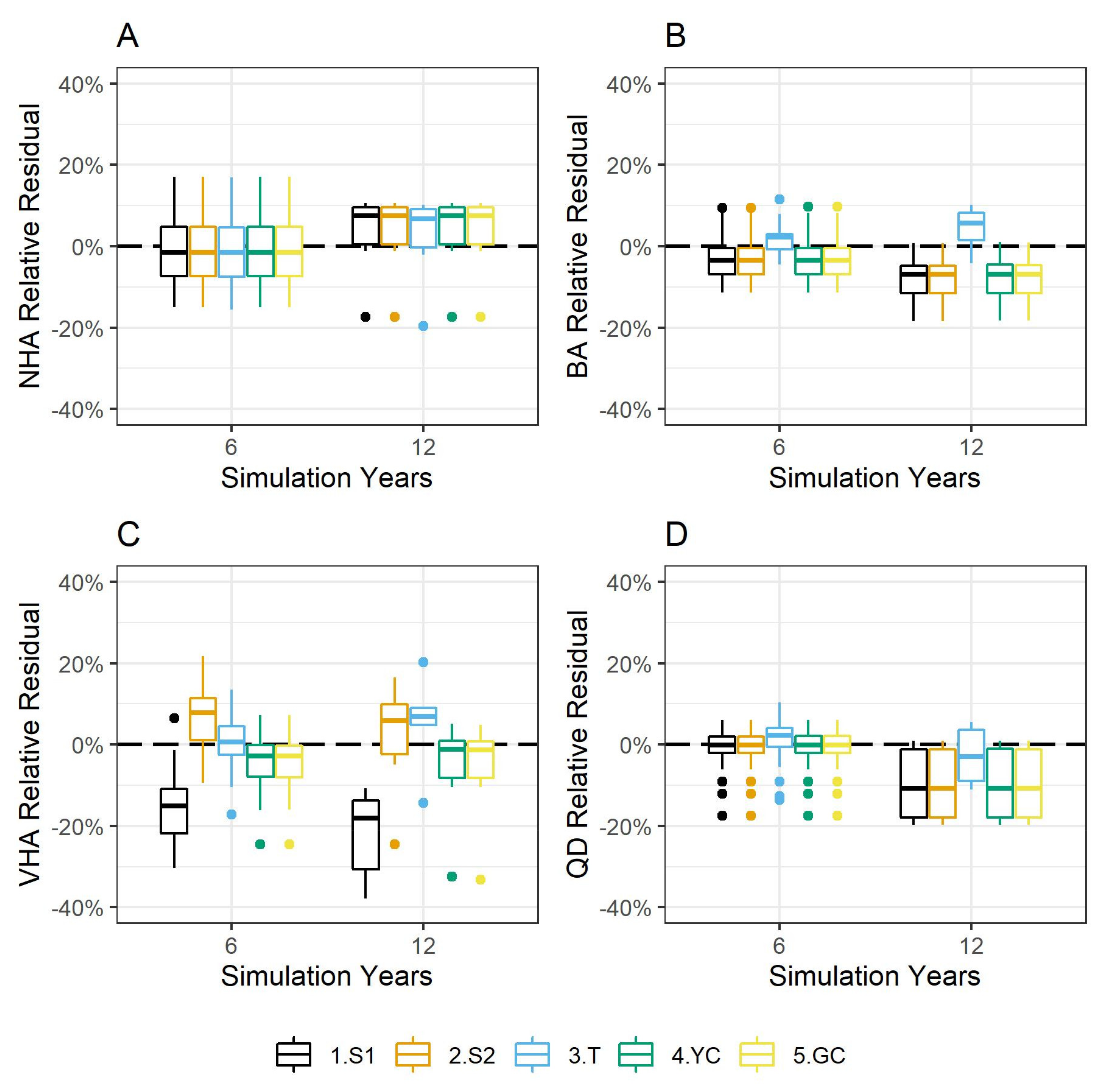
3.1. Number of Trees Goodness-of-Fit

The simulation models studied were stand-level without diameter distribution (S1), stand-level incorporating a generation of a diameter distribution (S2), tree-level (T), yield compatibility (YC), and growth compatibility (GC). These were assessed based on different goodness-of-fit measures for their predictions of stand parameters such as the BA, QD, and VHA (

Table 2. Goodness-of-fit statistics for each simulation (S1, S2, T, YC, and GC, see text for definitions) for number of trees (NHA, trees ha⁻¹), basal area (BA, m² ha⁻¹), stand volume (VHA, m³ ha⁻¹), saw-log volume (VOLP_SL, m³ ha⁻¹), pulpwood volume (VOLP_PW, m³ ha⁻¹), residual volume (VOLP_RES, m³ ha⁻¹), and carbon stock (C, tonnes C ha⁻¹). Statistics are presented at 6 and 12 years of projection in second-growth RORACO forests in southern Chile.

		Projection 6 Years					Projection 12 Years
Statistic	Parameter	S1	S2	T	YC	GC	S1	S2	T	YC	GC
R2emp	NHA	0.97	0.97	0.97	0.97	0.97	0.95	0.95	0.94	0.95	0.95
	BA	0.93	0.93	0.97	0.93	0.93	0.70	0.70	0.87	0.70	0.70
	VHA	0.28	0.85	0.94	0.90	0.90	−0.06	0.78	0.83	0.75	0.74
	VOLP_SL		0.80	0.98	0.94	0.93		0.92	0.99	0.77	0.74
	VOLP_PW		0.43	0.92	0.93	0.92		0.68	0.79	0.83	0.82
	VOLP_RES		0.88	0.95	0.95	0.95		0.90	0.89	0.85	0.87
	C		0.74	0.97	0.96	0.96		0.80	0.89	0.86	0.86
RMSE%	NHA	8.47	8.47	8.61	8.47	8.46	11.76	11.76	12.27	11.77	11.75
	BA	5.91	5.91	3.92	5.93	5.93	10.80	10.80	7.09	10.76	10.76
	VHA	23.97	11.03	6.85	9.02	9.08	28.98	13.31	11.56	13.93	14.23
	VOLP_SL		35.33	11.77	19.41	20.14		19.63	7.24	32.95	34.53
	VOLP_PW		22.07	8.49	7.76	8.09		21.78	17.77	15.65	16.31
	VOLP_RES		18.70	11.81	12.54	12.16		18.65	19.66	22.68	21.81
	C		16.71	5.60	7.00	6.95		16.92	12.35	13.89	13.99
BIAS%	NHA	−1.10	−1.10	−1.27	−1.11	−1.10	2.94	2.94	2.00	2.92	2.94
	BA	−3.05	−3.05	1.82	−3.01	−3.01	−7.86	−7.86	4.29	−7.76	−7.76
	VHA	−19.18	6.43	0.11	−4.34	−4.41	−23.69	1.51	5.05	−5.81	−6.04
	VOLP_SL		29.50	0.55	−10.27	−11.00		11.96	2.61	−22.37	−23.60
	VOLP_PW		−5.93	0.67	−0.48	−0.14		−6.74	7.65	6.26	6.67
	VOLP_RES		−9.86	−3.88	−3.35	−3.24		−0.43	2.05	1.90	2.65
	C		12.98	2.40	−2.76	−2.81		4.40	5.42	−6.69	−6.82
U2	NHA	0.07	0.07	0.08	0.07	0.07	0.10	0.10	0.10	0.10	0.10
	BA	0.06	0.06	0.04	0.06	0.06	0.10	0.10	0.06	0.10	0.10
	VHA	0.23	0.10	0.06	0.09	0.09	0.26	0.12	0.10	0.12	0.13
	VOLP_SL		0.27	0.09	0.15	0.16		0.15	0.06	0.26	0.27
	VOLP_PW		0.21	0.08	0.07	0.08		0.19	0.15	0.13	0.14
	VOLP_RES		0.16	0.10	0.11	0.11		0.15	0.16	0.18	0.18
	C		0.16	0.05	0.07	0.06		0.15	0.11	0.12	0.12

and Figure 2). As expected, all the simulations presented similar results for the NHA, given that all the simulations used the same mortality model. The relative residuals for the NHA show similar errors for the simulation models at 6 and 12 years of projection (Figure 2A). The R²_emp at six years presented a value of 0.97, and with 12 years, it suffered a minimal drop to 0.95. The RMSE% was 8.47 and 11.76% at 6 and 12 years of projection, respectively; but the simulation model, T, was slightly worse with 8.61 and 12.27%, respectively. The BIAS% was low for both projection years, observing a higher bias for simulation T but still with values close to zero. The Theil’s inequality coefficient (U2) shows values close to zero, indicating a high performance in predictions of the simulation models where they have similar behavior (Table 2).

3.2. Basal Area Goodness-of-Fit

In contrast to what is expected from the theory, where stand models should have better accuracies for BA than individual-tree models for long periods, the present T simulation resulted in better goodness-of-fit statistics. The R²_emp values of 0.97 and 0.87 were found at 6 and 12 years of projection for the T simulation model, while other simulations gave lower values of 0.93 and 0.70 for the same periods. The RMSE% reached errors less than 6% at six years of projection and errors close to 11% at 12 years, showing high performance in the prediction of growth in the basal area. The BIAS% was low, with values close to 3% at six years of projection and 8% at 12 years. For the BA, the T simulation had a smaller bias and different behavior, presenting an under-estimation bias, while the other simulations presented over-prediction biases (Table 2). The relative residuals exhibited similar errors for all the simulations, where the T simulation resulted in lower bias and an opposite behavior to the other simulations (Figure 2B).

The QD is obtained using the NHA and BA; thus, the analysis is similar to these precedent stand parameters. However, it is possible to observe a small error at six years of projection in all the simulations, which increased at 12 years. Almost no bias was found at six years, changing to some over-estimation at 12 years, where, in all cases, the T simulation was less biased (Figure 2D).

3.3. Volume Goodness-of-Fit

The observed volume growth reached in the PP was 8.81 m³ ha⁻¹ year⁻¹ with a 95% CI of [5.78, 11.83] at six years and 11.21 m³ ha⁻¹ year⁻¹ with a 95% CI of [7.25, 15.17] at 12 years. The VHA presented greater differences between the simulation models. As expected, S1 showed deficient performance, indicating that a general volume equation (Equation (8)) is not accurate enough to predict the behavior of this parameter in the validation sample available (Table 2, Figure 2C). In contrast to BA, volume is probably the best parameter for the tree-level simulation model where following each tree’s development leads to better stand volume estimations. This is reflected in the T simulation that showed lower errors and bias for both time projections, 6 and 12 years, reaching R²_emp of 0.94 and 0.83, RMSE% of 6.85 and 11.56%, and BIAS% of 0.11 and 5.05%, respectively.

Despite the added uncertainty in the generation of a diameter distribution and in the calculation of volume through these estimated diameter classes, S2 showed good predictions for both projection periods. At six years, S2 performed worse than the compatibility simulations, YC and GC; however, at 12 years of projection, S2 was more stable than the YC and GC simulations, and even presented lower bias than the T simulation model with values of 1.51 and 5.05% for 6 and 12 years, respectively. The compatibility simulations presented over-estimation bias against S2 and T that showed an under-estimation of VHA predictions (Table 2). Nevertheless, once observing the relative residuals, these simulations presented an error close to 0% at 12 years of projection, but the T simulations still presented the lowest prediction errors (Figure 2C). These differences in VHA become more critical when the tree volume is subdivided into different stem products.

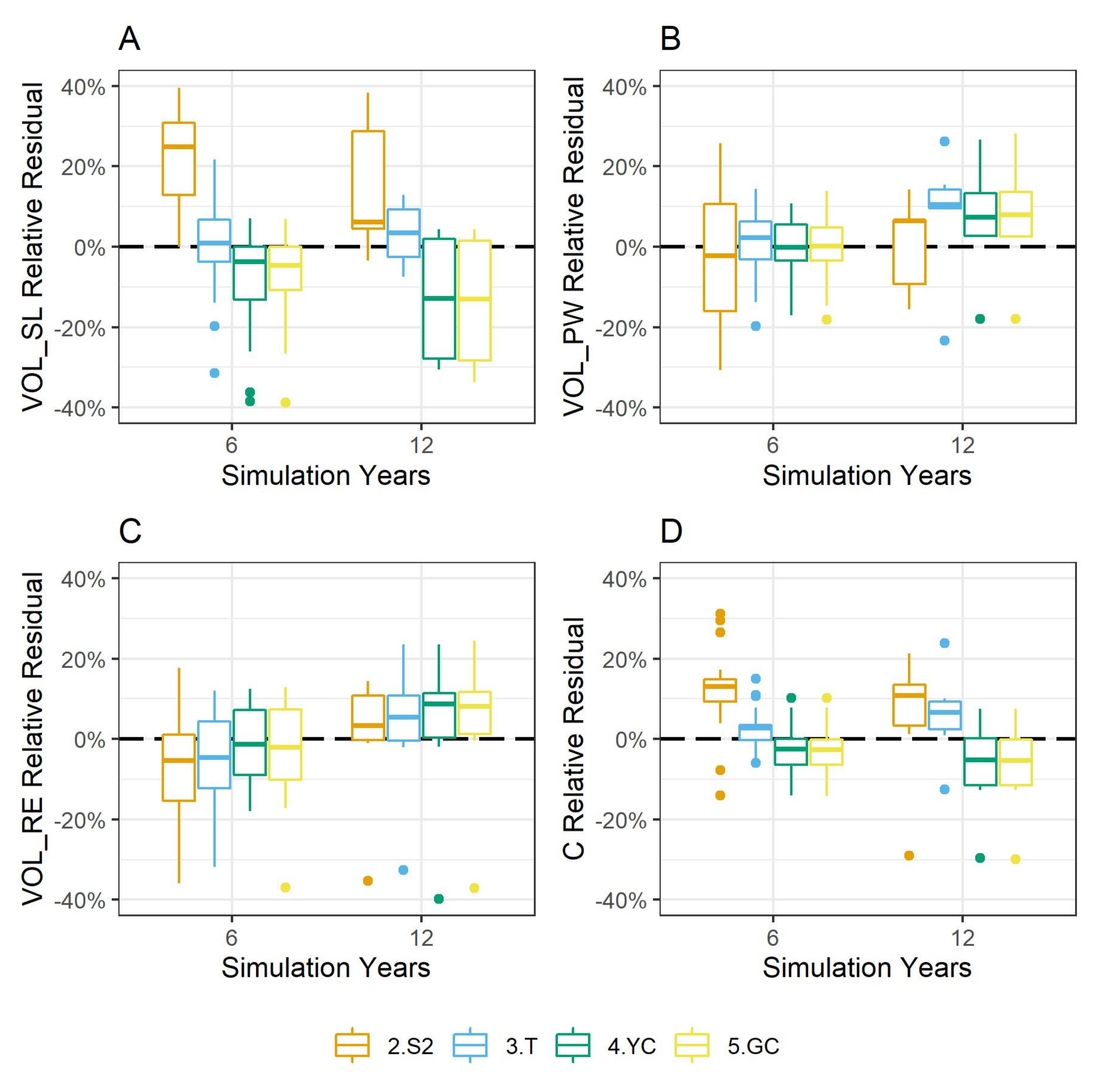
3.4. Products Volume Goodness-of-Fit

The following three objective products were defined to evaluate ecosystem services: saw-log (SL), pulpwood (PW), and residual lumber (RES). The simulation models’ performances were contrastingly different depending on the type of product and the projection time. SL, a product associated with higher income, was better predicted for by the T simulation with an excellent R²_emp of 0.98 and 0.99 at 6 and 12 years, respectively. The RMSE% was 11.77% at six years of projection, decreasing with 12 years to 7.24%. At the same time, the T simulation presented almost no bias at six years, marginally increasing to 2.61% at year 12. The U2 statistics were all close to zero, indicating a good prediction for saw-log volume (Table 2).

On the contrary, the S2 simulation model had deficient performance for predicting SL; here, both the RMSE% and BIAS% were more deficient at six years (35.33 and 29.50%, respectively) than at 12 years of projection (19.63 and 11.96%, respectively). The compatibility simulation models presented better predictions than S2 at six years, but their behaviors were worst at 12 years of projection, indicating a high-volume over-estimation. The Weibull distribution diameter model used in building the model for the S2 simulations had difficulties estimating the proportion of large trees, and therefore, under-estimates the log-volume for larger trees (those subject to a minimum diameter of 24 cm) (Figure 3A).

In the case of volume for the pulpwood product (PW), better simulation results were found for the compatibility models, where the GC was slightly poorer than the YC. However, the performance of the T simulation was similar to both compatibility models, having good statistics for R²_emp (>0.92 at six and >0.79 at 12 years), RMSE% (<8.5% at six and <17.8% at 12 years), BIAS% (<1% at six and <8% at 12 years), and U2 (<0.08 at six and <0.15 at 12 years). As occurred previously with SL, neither of the S2 simulations presented reasonable PW estimations. For example, its R²_emp value at six years was only 0.43; however, as with SL, the predictions improved at 12 years of projection with an R²_emp of 0.68 (Figure 3B, Table 2).

The volume for the residual lumber (RES) presented a more consistent behavior, where the T simulation showed a slightly overall better performance. For this product, all the simulations showed a decreasing BIAS% but an increased RMSE% at 12 years of projection (Table 2). The relative residuals showed similar trends as the goodness-of-fit statistics but with lower bias for the compatibility models at six years (Figure 3C).

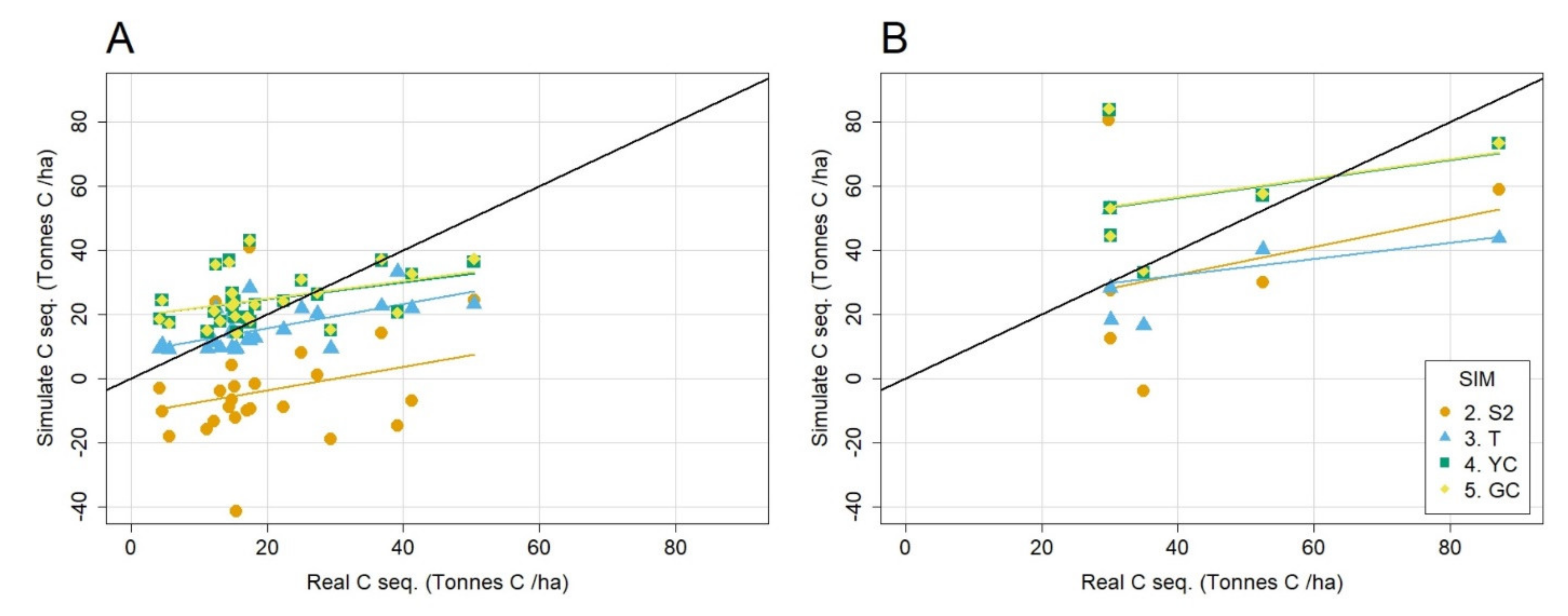
3.5. Carbon Stocks Goodness-of-Fit

In general, the predictions of carbon stocks presented good performance, where the T simulations showed better results with an R²_emp of 0.97 at six years and 0.89 at 12 years of projection. However, the compatibility simulations, YC and GC, showed similar statistics (0.96 and 0.86), for the same periods, respectively. Given that all the above-ground biomass equations (Equations (25)–(28)) used are strongly associated with the DBH and H, the S2 simulation had some difficulties to predict C, but still had reasonable accuracy with R²_emp values of 0.74 and 0.80 at 6 and 12 years, respectively (Table 2).

The statistic RSME% presented lower values at six years for the T, YC, and GC simulation models, but these doubled at 12 years of projection. In contrast, the errors of the S2 simulation stayed at ~17% for both periods, but these were still higher than other simulations. S2 and T presented an under-estimation for C, while the YC and GC presented an overestimation in both periods of projection (Figure 3D). However, the estimations were almost unbiased with values lower than 3 and 7% for both years of prediction, except for the prediction of C at six years using simulation S2 (13%).

The carbon sequestration observed for the growth period of six years was 19.82 tonnes C ha⁻¹ with a 95% CI of [14.98, 24.67]. In the case of 12 years of projection, the observed growth was 44.11 tonnes C ha⁻¹ with a 95% CI of [20.19, 68.02]. The CI interval for carbon sequestration over 12 years is an indication of the high variability found in the remeasured plots; thus, simulations have to be able to deal with these diverse natural conditions. The T simulation presented the best performance at six years, increasing its under-estimation as sequestration values got larger. This is probably due to issues with under-estimation arising from the mortality model, or otherwise, due to the absence of an ingrowth component in the simulations (Figure 4A). The compatibility models showed an over-estimation at smaller carbon sequestration levels (<25 tonnes C ha⁻¹) and showed better behavior with larger levels. The S2 simulation presented an under-estimation for the majority of the plots. Both simulations at 6 and 12 years of projection had similar behavior, but with more errors in the estimation at 12 years, as expected (Figure 4B).

4. Discussion

The model evaluations performed in this study, based on the data used for validation, suggest that stand level models, S1 and S2, present limitations for prediction, especially with volume (VHA). The use of the same mortality model for all the simulations allowed the isolation of its effects in the evaluation of the different simulation approaches. However, some problems associated with the prediction of other stand variables, such as the BA, VHA, QD, volume of products, and C stocks, could originate in the limited NHA predictions. Two important observations of this study are that these simulation models were fitted for Nothofagus species mainly, and they do not have an ingrowth module (hence, ingrowth is assumed to be zero). The model evaluations performed found problems in the NHA prediction once separated by species (N. alpina, N. obliqua, N. dombeyi, and companion species) (Figure 5). The companion species had a poor performance compared to the Nothofagus species, accumulating errors and bias over the prediction periods. In addition, it was detected in the inventory data that in 2012, a few trees belonging to the companion species were observed; however, this recruitment was not considered in any of the simulated models (Figure 2A). Nonetheless, given these limitations, the NHA presented, in general, an excellent performance with small errors and an almost null bias given that RORACO forests, by definition, are mainly composed of Nothofagus species.

In most G&Y models, it is expected that the basal area (BA), over long periods, will be better predicted by stand-level models [4,6,31] than by tree-level models; however, in the present study, S1 and S2 did not show good accuracy. On the contrary, the tree-level simulation presented better BA estimations, not only with lower errors but also with less bias. This improvement is likely due to the incorporation of individual tree-competition predictors, such as BAL or RS, that deal better with the future response of RORACO forests [16]. This performance in the T simulation also suggests that the individual DBH growth for RORACO stands is highly correlated with its current size (DBH and H), competition status, and site characteristics. Similar conclusions have been reported in other mixed-species forest G&Y models [32,33]. Additionally, it is possible that the accuracy of stand-level BA growth models is affected by the higher tree density (NHA) of companion species, adding not only more uncertainty in their BA growth but, as mentioned before, affecting mortality patterns [11].

In contrast to the T simulations, the poor BA estimation of the stand-level simulation models affected the compatibility simulation models as well, given that these are fixed to the stand-level BA estimation. It is expected that the compatibility models will result in improvements in the BA estimation at the tree-level, as they will match the BA estimated using stand-level models. However, in the present study, the T simulation had a better performance than the compatibility models, YC and GC. This result contrasts with improvements in individual volume predictions when using the proportional growth compatibility method, as reported for Douglas-Fir stands [34]. Nonetheless, the YC and GC methods showed similar performance in predictions for stand parameters, with the GC slightly poorer than the YC. Other contrasting results have been reported for birch [6] and loblolly pine plantations [23], where the predicted goodness-of-fit statistics for the BA were better using the GC than the YC method.

The high resolution of the T simulation (tree-level), as expected, led to a better prediction of stand volume (VHA). On the contrary, the whole-stand simulation, S1, presented a low capacity to accurately predict the VHA. Similar behavior has been reported in other species [7,35]. However, the inclusion of a generated diameter distribution, as conducted in the S2 simulation, increased the ability to accurately predict the volume per hectare, a result that agrees with other studies [7].

The volume disaggregation required to increase the accuracy in the economic evaluation of ecosystem services, including saw-log timber and pulpwood, together with carbon sequestration estimations, showed different behavior depending on the simulation model, time of projection, and specific output analyzed. The T simulation was more successful in the prediction of the saw-log timber volume (SL), a positive result associated with its higher resolution and capacity to model thicker stem diameters properly. For saw-log volume, the stability in the DBH growth model translated into relatively constant errors with a low bias at 12 years. All the other simulation models presented poorer estimations with high increases in the RMSE%. However, for the small diameters associated with pulpwood volume (PW), the compatibility models, YC and GC, presented a slightly better performance than the T simulation. The product estimation errors for S2 simulation are higher than for other simulations, but also, for those products with small diameters, such as PW and RES. Here, the prediction tends to have decreased errors as the projection period increased. Qin and Cao (2006) found the same behavior, where the stand-level simulations showed a tendency to produce more accurate estimates for long-term growth.

The ability to predict carbon stocks was directly associated with the prediction of VHA; thus, the T simulation had better accuracy for both projection periods. The compatibility simulations also had excellent predictions with a bias lower than 7% at 12 years of projection, indicating a good performance from these models. S2, despite presenting poorer goodness-of-fit statistics, is still capable of predicting C with a reasonable R²_emp value of 0.80 at 12 years of projection. However, S2 showed an underestimation at six years of projection, even simulating a bigger emission than the sequestration of C (Figure 4A). This underestimation was induced by the low capacity in volume prediction, a high rate of mortality modeled, and the lack of ingrowth simulation.

The observed annual carbon sequestrations in this study were, on average, between 3.3 and 3.7 tonnes C ha⁻¹ year⁻¹. Similar values were reported by Parada et al. [15] with 2.5 tonnes ha⁻¹ year⁻¹ for the carbon sequestration of above-ground tree dry matter biomass in a forest with the presence of the emergent N. dombeyi in Parque Nacional Puyehue, Chile. The values found in the present study indicate that the second-growth RORACO forest type, specifically the stands dominated by N. obliqua, are sequestering substantial amounts of carbon. However, due to the high variability found in the estimation of this variable, it is recommended, for studies focused on estimation of carbon sequestration for these forests, to use inventories with increased statistical power to reduce uncertainties.

As with any G&Y simulations, the compatibility adjustments, as well as the unadjusted predictions, suffer from an accumulation of errors and reduction in the goodness-of-fit statistics on their predictions as the simulation period increases. The compatibility methods are not only limited in their accuracy by the length of the simulation, but they are also strongly influenced by the accuracy of the stand-level simulations. Nevertheless, all the simulations evaluated had U2 values close to zero, indicating a better performance than the null hypothesis; that is, these models outperform the mean value estimation.

The sample of permanent plots used to validate the simulation models presented here incorporate the variability and different stand conditions of RORACO forests; however, these data are primarily dominated by N. obliqua, limiting inference to this forest type. Thus, there is a need for additional permanent plot data to validate further conditions and improve these models, particularly on the other two dominant species, N. alpina and N. dombeyi.

The G&Y system, packed in the R library Nothopack, to our knowledge represents the first effort to incorporate stand-level, individual-level, and compatibility models for the total distribution area of RORACO forests in Chile. The lack of time series or remeasured permanent plots limits this model, in aspects such as the incorporation of an ingrowth module or the inclusion of specific models for companion species. However, this is a dynamic process and further long-term data and evaluations should improve these aspects in the future, leading to an improved G&T system. In any case, this simulator is, without a doubt, a baseline for further improvements using and developing new models built with more robust information.

The implications of the results from Nothopack are useful for the sustainable management of second-growth RORACO forests in southern Chile, particularly given the importance and need of having some estimation of its value and a general idea of its management (thinning) that also includes some stimulus from the government. The principal users of Nothopack are small owners of these Nothofagus forests, forester consultants, and government agencies, as they require this type of tool to monitor the management of these resources, both for fiber products and ecosystems services.

5. Conclusions

The fitted individual-tree simulations show reasonably accurate predictions and a low bias for basal area, volume, specific products volume, and carbon stocks. The whole stand-level with the generation of a diameter distribution and both compatibility simulations displayed reasonable estimates, even with projections of 12 years. The present evaluations with independent remeasured plots confirm that the simulator Nothopack is a useful tool to support management plans for these forest ecosystems, where growth estimates might be limited to stands under 90 years old, or to merely update forest inventories over a short period (e.g., less than 10 years). Finally, this study provides the first evaluation and implementation of compatibility methods to link stand- and individual-level models in second-growth stands for RORACO forests in southern Chile.

References

1. Vanclay, J.K. Modelling Forest Growth and Yield: Applications to Mixed Tropical Forests; CAB International: Wallingford, UK, 1994; p. 537. [Google Scholar]
2. Porté, A.; Bartelink, H.H. Modelling mixed forest growth: A review of models for forest management. Ecol. Model. 2002, 150, 141–188. [Google Scholar] [CrossRef]
3. Vanclay, J.K. Synthesis: Growth Models for Tropical Forests: A Synthesis of Models and Methods. For. Sci. 1995, 41, 7–42. [Google Scholar] [CrossRef]
4. Qin, J.; Cao, Q.V. Using disaggregation to link individual-tree and whole-stand growth models. Can. J. For. Res. 2006, 36, 953–960. [Google Scholar] [CrossRef]
5. Cao, Q.V. Linking individual-tree and whole-stand models for forest growth and yield prediction. For. Ecosyst. 2014, 1, 18. [Google Scholar] [CrossRef] [Green Version]
6. Hevia, A.; Cao, Q.V.; Álvarez-González, J.G.; Ruiz-González, A.D.; Gadow, K.V. Compatibility of whole-stand and individual-tree models using composite estimators and disaggregation. For. Ecol. Manag. 2015, 348, 46–56. [Google Scholar] [CrossRef]
7. Shortt, J.S.; Burkhart, H.E. A Comparison of Loblolly Pine Plantation Growth and Yield Models for Inventory Updating. South. J. Appl. For. 1996, 20, 15–22. [Google Scholar] [CrossRef] [Green Version]
8. Zhang, X.; Lei, Y.; Cao, Q.V. Compatibility of Stand Basal Area Predictions Based on Forecast Combination. For. Sci. 2010, 56, 552–557. [Google Scholar] [CrossRef]
9. Cao, Q.V. An integrated system for modeling tree and stand survival. Can. J. For. Res. 2017, 47, 1405–1409. [Google Scholar] [CrossRef] [Green Version]
10. Blanco, J.A.; González de Andrés, E.; San Emeterio, L.; Lo, Y.H. Modelling mixed forest stands: Methodological challenges and approaches. In Advanced Modelling Techniques Studying Global Changes in Environmental Sciences; Lek, S., Park, Y.S., Baehr, C., Jorgensen, S.E., Eds.; Elsevier: Amsterdam, The Netherlands, 2015; pp. 187–213. [Google Scholar]
11. Palmas, S.; Moreno, P.C.; Cropper, W.P.; Ortega, A.; Gezan, S.A. Stand-Level Components of a Growth and Yield Model for Nothofagus Mixed Forests from Southern Chile. Forests 2020, 11, 810. [Google Scholar] [CrossRef]
12. Moreno, P.C.; Palmas, S.; Escobedo, F.J.; Cropper, W.P.; Gezan, S.A. Individual-Tree Diameter Growth Models for Mixed Nothofagus Second Growth Forests in Southern Chile. Forests 2017, 8, 506. [Google Scholar] [CrossRef] [Green Version]
13. CONAF. Catastro de los Recursos Vegetacionales Nativos de Chile, Monitoreo de Cambios y Actualizaciones, Periodo 1997–2011; CONAF: Santiago, Chile, 2011. [Google Scholar]
14. Millenium Ecosystems Assessment. Ecosystems and Human Well-Being: Synthesis; Island Press: Washington, DC, USA, 2005. [Google Scholar]
15. Parada, T.; Lusk, C.H.; Donoso, P.J. Evidence that emergent Nothofagus dombeyi do not depress carbon sequestration rates of canopy species in an old-growth Chilean temperate forest. N. Z. J. Bot. 2018, 56, 311–322. [Google Scholar] [CrossRef]
16. Moreno, P.C.; Gezan, S.A.; Palmas, S.; Escobedo, F.J.; Cropper, W.P., Jr. Exploring stand and tree variability in mixed Nothofagus second-growth forests through multivariate analyses. Bosque 2018, 39, 397–410. [Google Scholar] [CrossRef] [Green Version]
17. Avery, T.E.; Burkhart, H. Forest Measurements, 5th ed.; McGraw-Hill: New York, NY, USA, 2002. [Google Scholar]
18. Gezan, S.A.; Ortega, A.; Andenmatten, E. Diagramas de manejo de densidad para renovales de roble, raulí y coigüe en Chile. Bosque 2007, 28, 97–105. [Google Scholar] [CrossRef]
19. Gezan, S.; Moreno, P.; Palmas, S.; Ortega, A. NOTHOPACK: A Growth and Yield Simulator for Nothofagus Second Growth Forests. 2020. Available online: https://github.com/sgezan (accessed on 1 September 2021).
20. Reineke, L.H. Perfection a stand-density index for even-aged forest. J. Agric. Res. 1933, 46, 627–638. [Google Scholar]
21. Gezan, S.; Ortega, A. Desarrollo de un simulador de rendimiento para renovales de roble, raulí y coigüe; FONDEF D97I1065; Universidad Austral de Chile: Valdivia, Chile, 2001. [Google Scholar]
22. Gezan, S.A.; Moreno, P.; Ortega, A. Modelos fustales para renovales de roble, raulí y coigüe en Chile. Bosque 2009, 30, 61–69. [Google Scholar] [CrossRef]
23. Cao, Q.V. Predictions of individual-tree and whole-stand attributes for loblolly pine plantations. For. Ecol. Manag. 2006, 236, 342–347. [Google Scholar] [CrossRef]
24. CONAF. Manual Para el Manejo Forestal de Bosque Nativo. Available online: https://investigacion.conaf.cl/archivos/repositorio_documento/2018/10/manualManejoForestal.pdf (accessed on 15 July 2020).
25. Milla Araneda, F.; Emanuelli Avilés, P.; Sartori Ruilova, A.; Emanuelli Avilés, J. Compendio de Funciones Alométricas Para la Estimación de la Biomasa de Especies Forestales en Chile: Elemento Clave Para el Desarrollo de la Estrategia de Bosques y Cambio Climático (ENBCC); Corporacion Nacional Forestal: Santiago, Chile, 2013. [Google Scholar]
26. IPCC. 2006 IPCC Guidelines for National Greenhouse Gas Inventories, Prepared by the National Greenhouse Gas Inventories Programme; Eggleston, H.S., Buendia, L., Miwa, K., Ngara, T., Tanabe, K., Eds.; IGES: Hayama, Japan, 2006. [Google Scholar]
27. Gayoso, J.; Guerra, J. Contenido de carbono en la biomasa aérea de bosques nativos en Chile. Bosque 2005, 26, 33–38. [Google Scholar] [CrossRef]
28. Ahlburg, D.A. Forecast evaluation and improvement using Theil’s decomposition. J. Forecast. 1984, 3, 345–351. [Google Scholar] [CrossRef]
29. Welham, S.J.; Gezan, S.A.; Clark, S.; Mead, A. Statistical Methods in Biology: Design and Analysis of Experiments and Regression; CRC Press: Boca Raton, FL, USA, 2014. [Google Scholar]
30. R Core Team. R: A Language and Environment for Statistical Computing; R Foundation for Statistical Computing: Vienna, Austria, 2017. [Google Scholar]
31. Burkhart, H.E.; Tomé, M. Modeling Forest Trees and Stands; Springer Science & Business Media: Dordrecht, The Netherlands, 2012. [Google Scholar]
32. Monserud, R.A.; Sterba, H. A basal area increment model for individual trees growing in even-and uneven-aged forest stands in Austria. For. Ecol. Manag. 1996, 80, 57–80. [Google Scholar] [CrossRef]
33. Wykoff, W.R. A Basal Area Increment Model for Individual Conifers in the Northern Rocky Mountains. For. Sci. 1990, 36, 1077–1104. [Google Scholar] [CrossRef]
34. Zhang, L.; Moore, J.A.; Newberry, J.D. Disaggregating Stand Volume Growth to Individual Trees. For. Sci. 1993, 39, 295–308. [Google Scholar] [CrossRef]
35. Scolforo, H.F.; McTague, J.P.; Burkhart, H.; Roise, J.; Campoe, O.; Stape, J.L. Eucalyptus growth and yield system: Linking individual-tree and stand-level growth models in clonal Eucalypt plantations in Brazil. For. Ecol. Manag. 2019, 432, 1–16. [Google Scholar] [CrossRef]
Figure 1. Geographical location of permanent plots in second-growth RORACO forests in southern Chile established in 2000, with a first remeasurement in 2006 (n = 19) and a second in 2012 (n = 6). Growth zones defined for RORACO forests also are shown.
Forests 12 01236 g001
Figure 2. Stand parameters for each simulation (S1, S2, T, YC, and GC, see text for definitions). (A): number of trees (NHA, trees ha−1), (B): basal area (BA, m2 ha−1), (C): stand volume (VHA, m3 ha−1), and (D): quadratic diameter (QD, cm). Statistics are presented as box plots of relative residuals at 6 and 12 years of projection in second-growth RORACO forests in southern Chile.
Forests 12 01236 g002
Figure 3. Ecosystem services for simulation S2, T, YC, and GC, see text for definitions. (A): saw-log volume (VOLP_SL, m3 ha−1), (B): pulpwood volume (VOLP_PW, m3 ha−1), (C): residual volume (VOLP_RES, m3 ha−1), and (D): carbon stock (C, tonnes C ha−1). Statistics are presented as box plots of relative residuals at 6 and 12 years of projection in second-growth RORACO forests in southern Chile.
Forests 12 01236 g003
Figure 4. Carbon sequestration at six (A) and 12 (B) years of projection in second-growth RORACO forests in southern Chile for each simulation model. Solid black lines represented the one-to-one line between observed and predicted values. Solid color lines are the fitted regression for each of the simulations S2, T, YC, and GC (see text for definitions).
Forests 12 01236 g004
Figure 5. RMSE% (black, RMSEp) and BIAS% (red, BIASp) for number of trees (NHA, trees ha−1) at 6 and 12 years of projection in second-growth RORACO forests in southern Chile. Statistics are presented by species (NA, N. alpina; NO, N. obliqua; ND, N. dombeyi; OT, companion species) and by simulation model (S1, S2, T, YC, and GC, see text for definitions).
Forests 12 01236 g005