Article

Multispectral Spaceborne Proxies of Predisposing Forest Structure Attributes to Storm Disturbance—A Case Study from Germany

Environmental Meteorology, University of Freiburg, Werthmannstrasse 10, 79085 Freiburg, Germany
*
Author to whom correspondence should be addressed.
Forests 2022, 13(12), 2114; https://doi.org/10.3390/f13122114
Submission received: 15 November 2022 / Revised: 7 December 2022 / Accepted: 8 December 2022 / Published: 10 December 2022
(This article belongs to the Section Forest Inventory, Modeling and Remote Sensing)

Abstract

:
Windstorms are among the primary drivers of forest disturbances. Although they are inherent part of the natural ecosystem processes, they severely impact managed forests. Modeling approaches serve as key tools for the evaluation of disturbance risk and different predisposing factors. However, data availability on relevant forest attributes can be problematic on a larger scale. While spaceborne remote sensing has already proven itself as a tool for disturbance detection, its use in relation to predisposing forest attributes remains underexploited. The present work explores multispectral object-based proxy predictors for statistical wind disturbance modeling based on the publicly available Sentinel-2 imagery and recorded damage polygons from the pan-European FORWIND database. Potential predictors were tested in logistic and random forests (RF) regression models for both disturbance occurrence and severity for a case study of a major storm event in Northern Germany from 2017. The results reveal a general potential of the derived spaceborne variables to be used as proxy variables to critical predisposing forest attributes. The presented proxy variables also outperformed a set of publicly available derived spatial data products for modeling both disturbance occurrence and severity. Model accuracies were moderate (reaching AUC = 0.76 for logistic regression fit and AUC = 0.69 for predictive accuracy of RF models), yet falling within the range of reported results in previous studies from the field. Limitations of the spectral satellite imagery as a single information source were acknowledged; however, the results indicate the further potential of spaceborne imagery applications in disturbance modeling, assessment and resulting mapping of disturbance susceptibility at different spatial scales. Considering the growing spatiotemporal availability of high-resolution spaceborne data, we propose that a model representation of post-disturbance forest patterns could improve the understanding of complex disturbance regimes and recurrent susceptibility.

1. Introduction

Storms and extreme winds are responsible for a significant share of recurrent forest disturbance in Europe and globally. In combination with other climate change-induced weather extremes and disturbance agents, the frequency and severity of catastrophic storms may increase in many parts of the world [1,2]. Trends of increased storminess are already identified and foreseen in Western and Central Europe [3,4,5], where increasing average forest age, height, growing stock, and historic management regimes can also amplify their consequences remarkably [6,7].
Although wind-related disturbance regimes are important drivers of the natural succession dynamics from stand to landscape level in various types of forest ecosystems [8,9,10], they have a strong negative impact on managed forests [11], including potentially reduced carbon storage capacities and an altered carbon balance at different timescales as a growing concern [1,12]. Detection of past disturbances, assessment and evaluation of recurrent wind damage are thus topics of high importance [6,11,13,14].
In Europe, windstorm events with the most severe disturbance intensity occur usually from November until March, associated with Atlantic atmospheric pressure regimes, affecting some regions more frequently than others, also in line with the observed increasing trends in Northwest Europe [14,15]. Beyond wind macroclimate, disturbance risk depends on several site and forest conditions. Some of the most important predisposing factors include topographic exposure (also as a primary driver of local wind patterns and properties), soil characteristics and wetness, rooting conditions, species composition, tree height and stand vertical structure, and past silvicultural activities such as thinning [13,16,17,18,19]. Regarding the meteorological driver, maximum wind gusts are reported to correspond best to disturbance occurrence and severity [20,21]. However, other wind characteristics for the duration of the storm events and local wind climate facilitating tree acclimation can also play an important role [13,14,22,23].
Considering both the significant and often detrimental effects of storms on managed forests and the influence of management practices on storm damage susceptibility at the same time, disturbance-aware forest management strategies can be crucial in the wind damage-prone areas and regions [13,24,25]. Improving the understanding of natural disturbance regimes can also enable their better integration into management strategies [10]. From both perspectives, modeling approaches serve as essential tools. The two main types of disturbance (or damage) models include statistical–empirical and mechanistic models [10,11,23,25,26,27]. In both types of models, a wide range of the earlier presented contributing factors are considered and represented as predictor variables, either at the individual tree or the stand level [17,23,26,27,28,29].
Despite recent and continuous model improvements, a lack of accurate predictors can still be a major concern at different scales. Availability of ground-measured forest attributes over larger areas and in a homogenous and area-wide manner raise concerns, despite existing forest inventories and the networks of in situ measurements used in some previous works [19,28,30,31,32]. Turbulence over forest canopies and fine-scale wind properties are also unrepresented in available meteorological records in general [23,33,34,35]. These, together with the inherent features of the applied models, make transferability and generalization of locally trained models to other and larger areas problematic [27,36,37]. In addition, it is also noted that the assessment of individual predisposing factors can be misleading in a generalized case [13].
For assessing wind damage risk and its underlying factors, reliable information on past and recent wind disturbances is also crucial and marking another challenging field [6,13,14]. To this end, remote sensing techniques, including satellite imagery, have been widely used. Approaches of satellite remote sensing have shown good accuracy, both for detecting and delineating disturbed areas [38,39,40] and for assessing the severity of disturbance events [41,42].
Satellite imagery, however, could potentially be used in a multifold way in relation to wind disturbances. This may include analyzing both the pre- and post-disturbance state of affected areas, linking predisposing factors to them and enabling the (up)scaling of the identified attributes frequently referred to as a great potential of remote sensing applications [43,44]. Analyzing canopy closure and structural features and their post-disturbance changes could also serve with valuable information on potential and recurrent wind damage susceptibility and could contribute to the understanding of less represented turbulent wind properties over forests [45]. Spatial patterns derived from higher resolution imagery, with a view on the methods of image texture analysis, can be also efficiently used in connection to disturbance assessment [46]. Nevertheless, growing availability and spatiotemporal coverage of suitable remote sensing data may also enable its potential direct use for disturbance modeling and deriving predictor variables.
Building on such considerations, the present study aims to further explore the utility and added value of remotely sensed spatial forest attributes as potential predictors in empirical wind disturbance models, using the growing archives of the Sentinel-2 multispectral imagery. The statistical relationship of the selected attributes to both disturbance occurrence and severity was evaluated, serving also with novel insights on the extension of previous modeling tools of disturbance occurrence. The performance of the proxy variables was compared to variables from available large-scale spatial data products selected as reference (benchmark) data sources. A case study of a significant storm event in Northern Germany from 2017 was selected and analyzed, taking advantage of the FORWIND database [14]. Concerning the limitations of the spaceborne spectral data in relating it unambiguously to specific forest attributes [47], the predictor variables presented in this study were handled and interpreted as general proxy variables to large-scale predisposing forest attributes, without their detailed further specification at the stage of this exploratory case study.

2. Materials and Methods

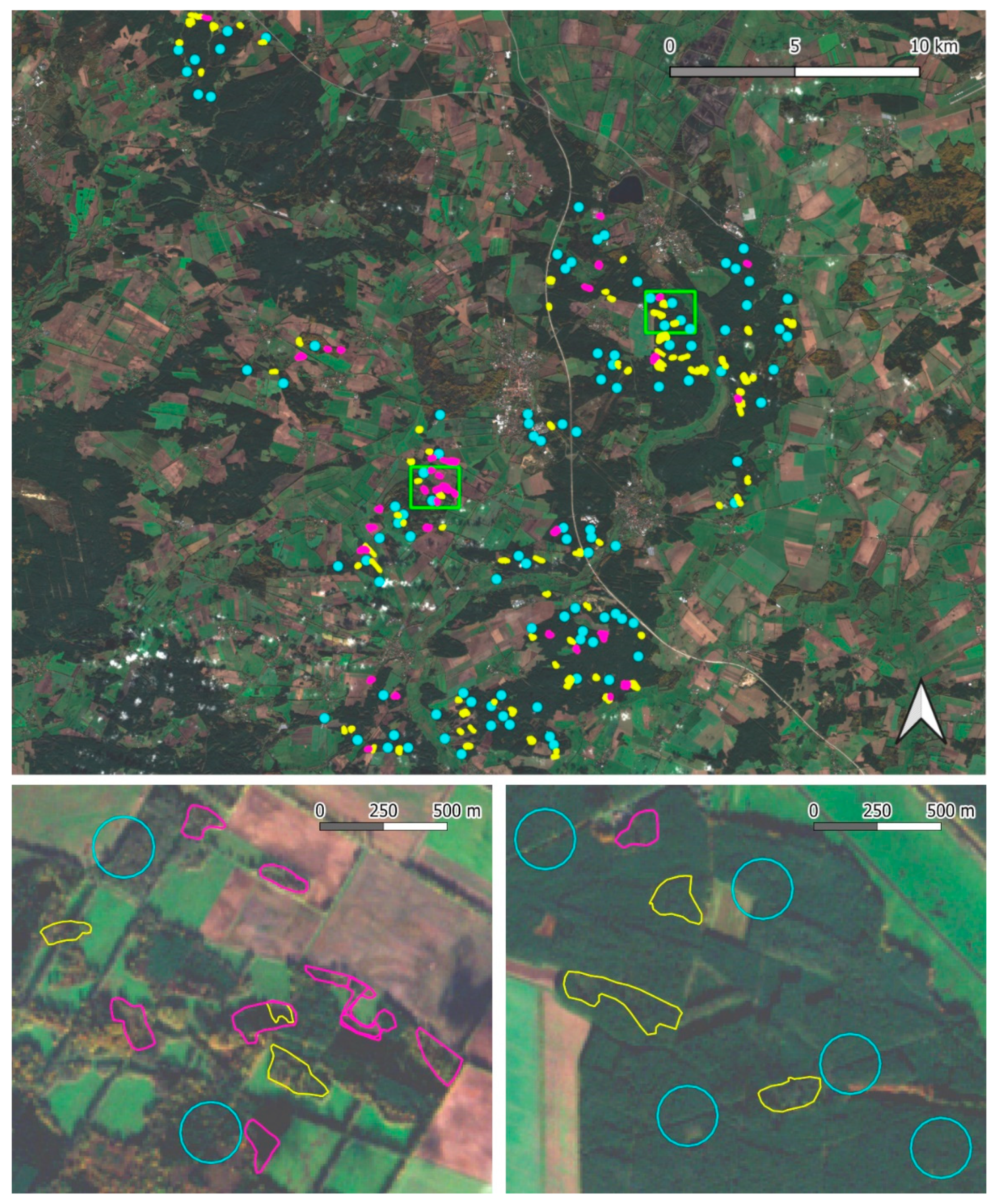
2.1. Study Area and Storm Disturbance Data

The recently published FORWIND database of storm disturbance events in European forests during the period of 2000–2018 served as the basis for the selection of the case study, with affected sites delineated in GIS vector polygon format [14]. In the case of a few events, the quantified damage degree (DG) within the delineated polygons (values between 0 and 1) was also available in the database, essential also for the area-based modeling of disturbance severity. From the major recorded disturbance events in European forests since the availability of the used satellite imagery, such information was available, among a few others, for the Atlantic-origin winter storm Xavier from Germany in 2017 [48]. This disturbance event was selected as a case study. The location and overview of the study area and affected forest sites are shown in Figure 1 (and more detailed in Figure A1).
Storm Xavier severely hit a region in the federal state of Mecklenburg-Vorpommern in Northern Germany on 5 October 2017 characterized by a maximum wind gust of 32.5 m/s [48,49]. This study area comprises forest stands at low elevations and flat terrain of floodplains and low hills, with the average elevation ranging from 23 to 76 m a.s.l. for the recorded damage polygons, corresponding to 556 ha of total disturbed area [14]. The forests are dominated by Scotch pine (Pinus sylvestris), with a smaller share of mixed and broadleaved stands characterized by the species of European beech (Fagus sylvatica) and pedunculate oak (Quercus robur). The share of conifers was estimated to be 72% in 2015 by remote sensing-based sources [50]. Xavier mainly left scattered single-tree damage and fewer areal windthrows behind, as recorded by an aerial photo interpretation of the local forestry authorities [49].
To enable working with more comparable pixel-based spatial statistics of forest plots with similar size, damage polygons with a size between 1 and 6 ha were selected from the dataset. Attention was also paid to the fact that this filtering did not result in bias of their original spatial and DG distribution, assured by visual checks of their spatial coverage and comparing histograms of DG distributions.
The sizes of the selected polygons broadly match the forest compartment sizes in Central Europe with individual management relevance [49,51]. However, they did not inherently share their borders with forest compartments nor indicate homogenous forest conditions by definition. Building on a general model selection approach of previous studies both for single tree and areal wind damage modeling [17,23,27], DG was reclassified as a binary variable of lower and higher damage. This was also desirable following less promising preliminary attempts to fit linear regressions, supported also by previous results [52].
Given the size (A) distribution patterns of damage polygons, their filtering was a convenient solution for this case study, excluding small (A < 1.0 ha, n = 1946; from which A < 0.5 ha, n = 1829) and a few larger polygons being outliers in their size (A > 6.0 ha, n = 7). This pre-selection left 120 disturbed forest plots for further analysis, with a corresponding disturbance severity range from DG = 0.25 to a single case of DG = 0.95, showing a strongly skewed distribution towards the lower DG values. Most of the recorded damage degree values were DG = 0.25, representing a categorical DG value associated with scattered individual tree damage, the lowest recorded DG value for this storm event within the dataset [14,49]. This also served as the premise of the binary categorization of the polygons by DG = 0.25 as very low (DG0; n = 85) and DG > 0.25 as significant damage (DG1; n = 35). Most records of the DG1 category fall between the range of 0.25 < DG < 0.60 (n = 32).
Previous wind disturbance modeling studies focused mainly on a binary differentiation of damaged or non-damaged trees and forest areas [17,23,27]. Besides the FORWIND disturbance polygons, a set of 105 reference polygons (NDG) in non-disturbed forest areas but within the vicinity of the disturbed sites were also delineated for the analyses. The mid-points of the circular NDG polygons with a radius of 120 m (and an area of ca. 4.5 ha) were randomly selected within a distance of 120 to 1000 m to the FORWIND polygons (Figure A1). The selection and delineation of the reference polygons were conducted by using the buffer and random points functions under the QGIS environment [53] on an intersection with a forest cover reference map derived from Copernicus Forest Type (FTY) 2015 product [50]. The analyzed total of 225 disturbed and reference forest polygons are also referred to as sample polygons hereafter.

2.2. Data Sources of Potential Predisposing Factors

Sentinel-2 (S2) satellite imagery was found as an outstanding, publicly available source for our work. S2 is a high-resolution multispectral imaging mission of the Copernicus Programme and the European Space Agency with a global equatorial 5-day revisit frequency. It consists of two satellites, with its first launch in June 2015. The S2 Multispectral Instrument samples in 13 spectral bands: visible and near-infrared (NIR) bands at 10 m, red-edge and short-wave infrared bands at 20 m and other atmospheric bands at 60 m spatial resolution. The resolution of 10 m (and partly of 20 m) was supposed to be fine enough to detect characteristic structures at the forest canopy level, even when not enabling sharp delineation of features at a scale of individual tree crowns [43,44,46].
Surface-level, geometrically and atmospherically corrected S2 images (level-2A, L2A) were downloaded from the Google Earth Engine (GEE) platform without the need for further pre-processing [54]. The GEE platform also facilitated a convenient selection of potential acquisition dates and clipping of downloaded images to the study area. Due to the frequent cloudiness during seasons with convective or frontal atmospheric regimes, a relatively scarce availability of reasonably cloud-free images was found before the storm event despite the regular and frequent revisit time of the S2 satellites [14,39]. Another reason for the relative scarcity in the number of potential images was due to the second S2 satellite (Sentinel-2B) imaging becoming only operational and available on the GEE platform in desired L2A format during the same year of data acquisition.
Multiple pre-disturbance images were selected to specify potential predictor variables for a robust statistical analysis. Considering reflectance bias due to different solar illumination angles and seasonal meteorological and vegetation conditions [39,51], four images before the disturbance event were selected. These included preferably cloud-free images at different phenological phases from 25 May 2017, 9 July 2017, 15 August 2017, and 17 September 2017.
Several spectral bands, including visible, red-edge, and NIR bands, were found previously as good indicators in vegetation and disturbance-related applications [39,46]. S2 images were downloaded at the spectral bands of red (B4, ~649–680 nm), green (B3, ~541–577 nm), blue (B2, ~459–525 nm), red-edge (B6, ~732–747 nm), and NIR (B8, ~780–886 nm). Although derived multispectral indices such as the normalized difference vegetation index were also used by some studies concerning wind disturbances [14,41], they were not included in this work, considering previous results suggesting no superiority of their spatial-oriented usage compared to individual spectral bands [46]. Due to its less specific information content over forests and vegetation, the blue band was used only for RGB visualization.
Besides the first-hand S2 data, meteorological, geographical, and other publicly available derived spatial data products were also included in the analyses, serving also as reference (benchmark) datasets. Modeled maximum gust speed was also available for the storm Xavier from the GeWiSA winter storm atlas at a spatial resolution of 25 m [48]. Although topography and topographic exposure are important predictors in most wind damage modeling studies over heterogeneous terrain [16,17,23,52,55], the topographic properties of the study area did not demand complex descriptors of them. The European digital elevation and topographic model available from the Copernicus website at a spatial resolution of 25 m [56] was used to quantify mean elevation of the sample polygons, similarly to the GeWiSA product.
A broader classification of coniferous and broadleaved forests and unstocked areas and estimated forest density were available from the 20 m resolution gridded datasets of the Copernicus pan-European FTY 2015 and Tree Cover Density (TCD) 2015 products, derived from S2 and Landsat imagery [50]. These products also indicated a few unstocked areas within the analyzed polygons. Timing and intensity of past scheduled silvicultural measures, including thinning, were, however, not expected to be available in an explicit manner over the study area. Further background information on tree species composition was derived from the literature dealing with the selected disturbance event [14,49], and partly from visual interpretation of the satellite images.
Although soil conditions such as rooting depth or soil wetness can be also crucial predisposing factors to wind disturbances [13,17,27,57], these were not directly addressed in the present work. However, considering a broad relationship of such soil attributes with topography, exposure, climate, and meteorology of the actual weather event, they can also be rather case study-specific and thus partly covered by the areal selection [30].

2.3. Processing of Spatial Data to Model Variables

Visualization and further processing of S2 images and other spatial data products and deriving object-based variables were done under the QGIS environment. A list of potential predictor variables was pre-selected (Table 1) based on the spectral S2 images (S2 variables/predictors) and the reference data products. These were calculated as object-based spatial variables both within the sample polygons and also separately in their 60 m wide buffer zones, excluding wind and topographic variables. The buffer width was set to be comparable with wind exposure related gap widths or distances from forest edges used in previous studies [27,30], and also to yield buffer zones with a sufficiently high number of full S2 pixels for the calculation of variables, similarly to the sample polygons.
Visible band reflectance showed a remarkable seasonal variability along the phenological changes as expected, but also the red-edge and NIR band reflectance depicted some less systematic and significant changes over time. Thus, S2 images from the four pre-disturbance acquisition dates were merged into single-band mean composites for the purposes of variable calculation. Due to scattered cumulus cloud pixels still being present on a few selected S2 images, some pixels were excluded from deriving the composite means at the respective acquisition dates. Pixel exclusion was conducted based on the visual evaluation-based criteria of maximum red and green pixel values exceeding a threshold of 1000 over forest pixels.
Spatial means of red (B4), green (B3), red-edge (B6), and NIR (B8) band pixel values of scaled surface reflectance were calculated first for each sample polygon using the zonal statistic function of QGIS. Beyond the pixel-based spectral reflectance, texture-related spatial patterns were also desired to be represented among the S2 variables [46,58]. To this end, spatial means of reflectance-based surface roughness of each four selected spectral band were included in the list of potential variables, using a moving kernel approach (with k = 3) for calculating the differences between neighboring pixels [59].
Polygon-wise means of the modeled maximum gust speeds (mWG), mean elevation (Elev), and mean tree cover density (TCm) were calculated similarly as the S2-based variables. Number of pixels from each three classes of the FTY 2015 data was calculated with the zonal histogram function within the sample polygons and their buffer zones. Among possible combinations, the share of unstocked pixels (NSr) and the share of broadleaved forest pixels among all forested pixels (BLr) were derived as potential predictor variables. These variables, based on public spatial data products, are also referred to as benchmark variables hereafter, in line with their usage in the subsequent analyses.

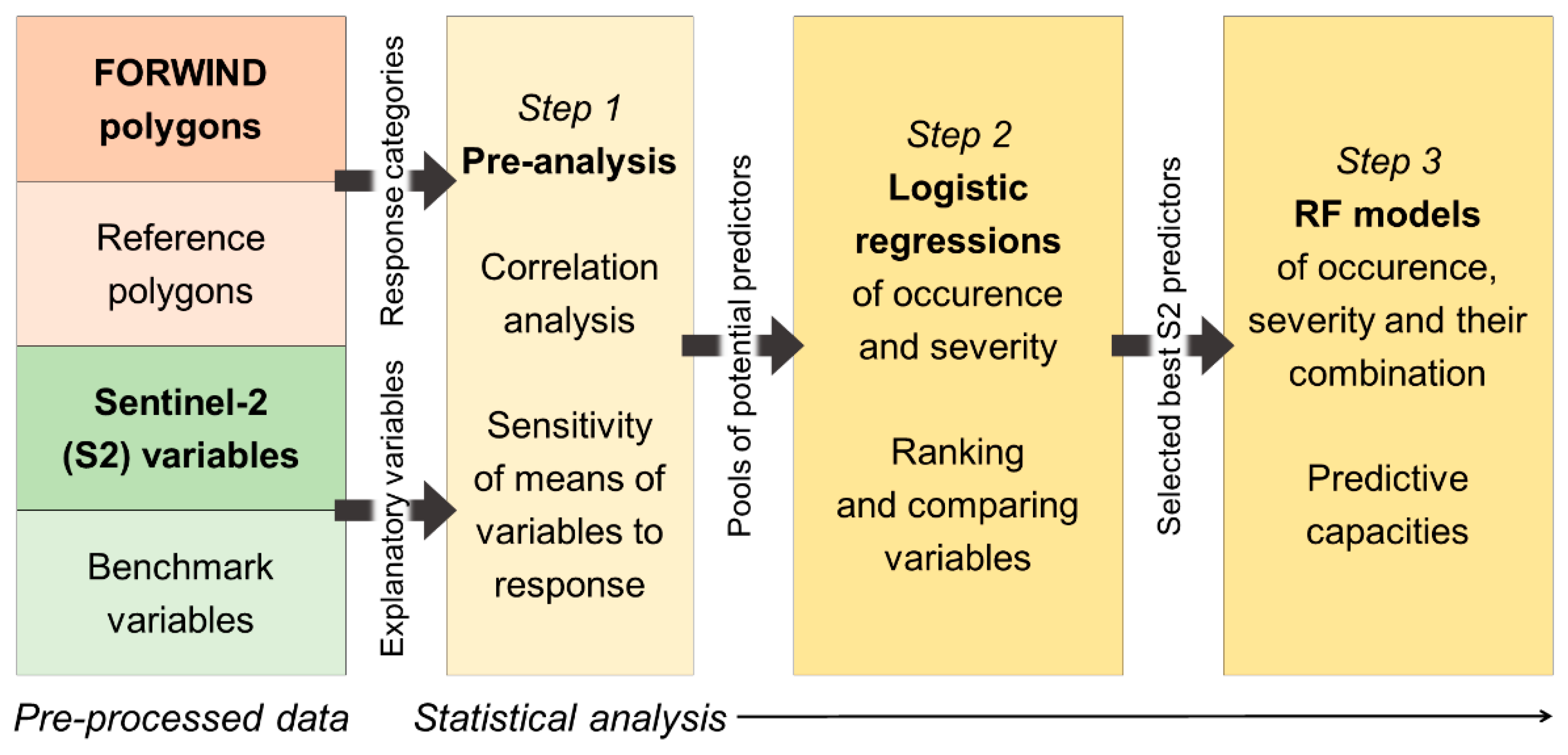
2.4. Statistical Analysis and Modeling

Data analysis and disturbance modeling were conducted in three consecutive steps, each building on the previous steps (Figure 2). First, collinear groups of S2 variables were pre-selected through a Pearson correlation analysis to avoid a simultaneous use of highly multicollinear predictors. Due to the inherent low-frequency spatial correlation between spectral reflectance values, a higher mean correlation coefficient threshold of | r | = 0.75 was used compared to other studies [2,23]. At the same stage, correlations between the FTY and TCD 2015 variables were also checked, together with their correlation to the S2 variables, facilitating also their interpretation.
A general sensitivity assessment of all listed variables to different disturbance categories also supported the predictor selection. This was conducted by pairwise Welch’s two-sample t-tests of the respective means [60], comparing non-disturbed to disturbed (NDG and joint DG0-DG1), and different damage severity categories (DG0 and DG1). Due to the high collinearity of S2 variables, their entire pools were assessed as potentially sensitive when several variables from them yielded significant t-test results.
At a second step, based on the defined collinear groups and their sensitivity to disturbance classes, the relationship of the selected variable (groups) with (1) disturbance occurrence and (2) binary DG categories was explored using logistic regression analysis. This statistical model represents a widely used tool in the wind damage modeling literature [23,27,29,36,37], offering also a detailed and straightforward comparative evaluation of the explanatory variables. Logistic regressions were fit separately for the S2 variables and the benchmark variables (reference regression fits) at the premises of generalized linear models (‘glm’ function) under the R statistical environment [61]. For the regression fitting, all variables were previously standardized by the statistical program.
All possible combinations of the S2 variables from the selected collinear pools were tested in regression fits respective to modeling both disturbance occurrence and severity, and ranked by the Akaike information criterion (AIC). Predictors for the final reference models were selected by the t-test results and expert judgement, based also on previous wind disturbance modeling literature. Benchmark variables with weak explanatory power were stepwise omitted to minimize AIC of regression fit until not corrupting the overall regression performance. Since an assessment of the proxy S2 variables and their comparative selection was a core purpose of the regression analysis, the entire sample size of polygons was used simultaneously for this part of the analyses, without the cross-validation of the predictive strength of the variables.
The assessment of the predictors was based on the z-values, estimating also their individual importance. Comparing z-value statistics enabled a more detailed assessment of the S2 predictors selected within the best five AIC-ranked logistic regression fits, indicating both their significance and characteristic sign of relationship to disturbance. The overall regression strength was indicated by the area under the curve (AUC) measure, used also elsewhere in the absence of general performance statistics for logistic regression [23,62]. The AUC measure was calculated for the best-ranked S2 and benchmark variable-based regression fits, using the ‘pROC’ package under R [63].
At a third and final step, the predictive capacity of the S2 variables was tested beyond the previous logistic regression analysis, using random forest (RF) models representing a flexible machine learning approach increasingly used for wind damage and other forest disturbance modeling [2,23,27]. Single RF models were applied for modeling disturbance occurrence and severity separately and for a combined differentiation between NDG, DG0 and DG1, built with the ‘randomForest’ package in R [64]. Here, a set of the best S2 predictor variables was used, based on their selection frequency and significance within each five best AIC-ranked logistic regression fits. All standardized predictors were used simultaneously in this method, considering the excellent capability of RF models to handle multicollinearity [23]. Models were built on 70% and tested on 30% of data in each model setting, randomly selected from distinct pools of the binary damage categories. RF models were built with default regression parameter settings of the ‘randomForest’ function and ran three times to calculate the AUC performance metric and the relative importance of the predictors. Using the regression parameter settings of the RF models, performance metrics were computed in line with similar modeling studies [23,27] and not directly aiming at a spatial classification or potential mapping of disturbance susceptibility.

3. Results

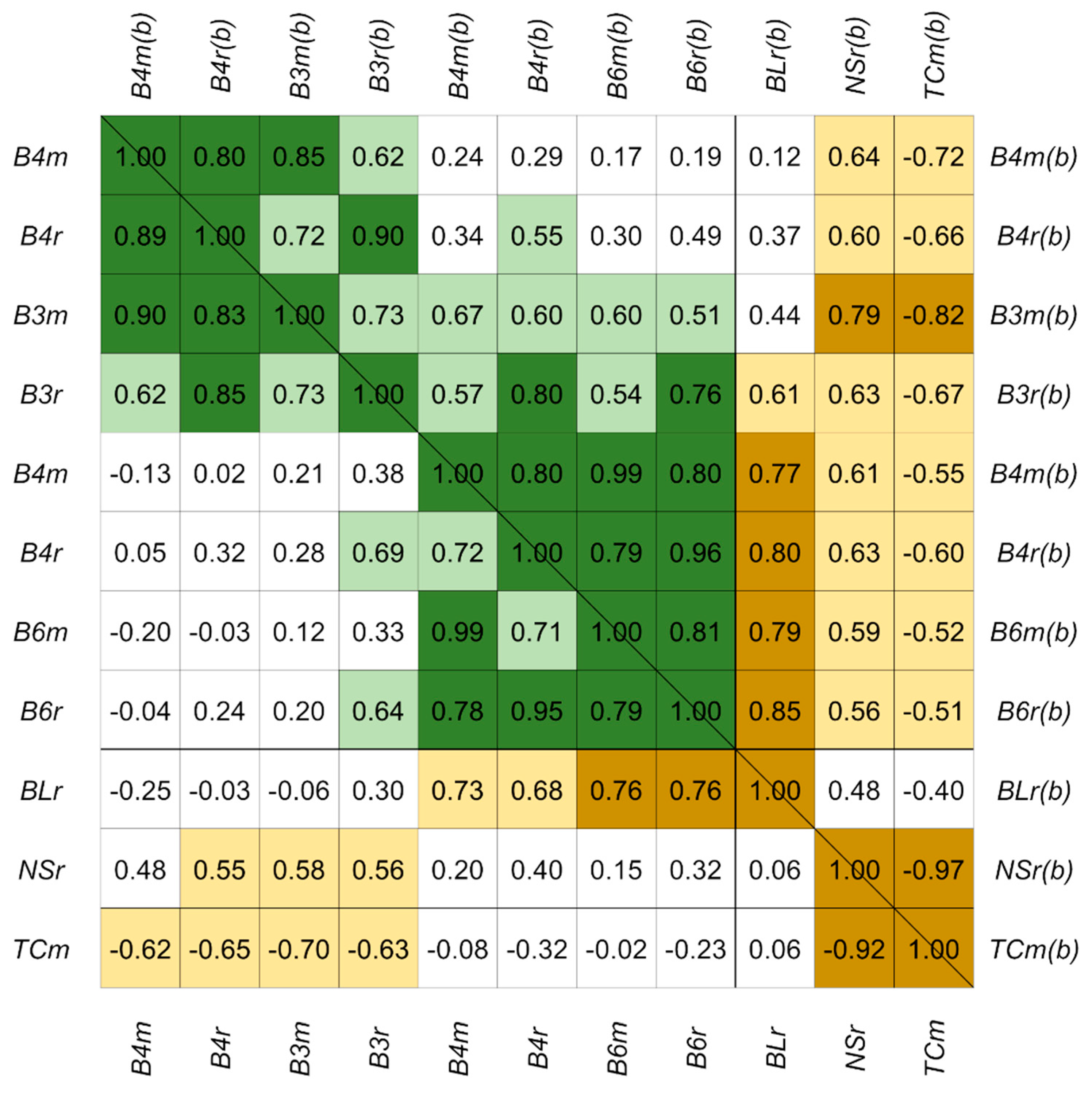
3.1. Correlation and Usage of Predictor Variables

Correlation analysis of the S2 variables revealed a principal differentiation between the visible and the group of red-edge and NIR bands (Figure 3). Yet the green-band variables, especially the green-roughness (B3r), showed a stronger relationship with the red-edge and NIR band variables. This was even more pronounced for the buffer zones of the sample polygons. Nevertheless, based on these outcomes, the visible band and the group of red-edge and NIR band variables were associated as the two main collinear S2 variable groups with correlation coefficients between variable pairs exceeding, on average, the threshold of | r | > 0.75 within each group.
The two main collinear groups also demonstrated different relationships to the variables derived from FTY and TCD 2015. In general, the visible band variables correlated positively with NSr and negatively with TCm (in most cases with | r | > 0.5), which two variables were also highly negatively correlated themselves (r < –0.9). In contrast, the red-edge and NIR variables showed very strong positive correlation with the share of broadleaved species (BLr; r > 0.6), but also a considerable relationship was detected between them and the variables NSr and TCm in the buffer zones (| r | > 0.5). The variable B3r exhibited somewhat different relationships compared to other visible band variables, being more correlated with BLr, especially within the buffer zones.
Comparing the difference in means for all selected variables (S2 and benchmark), their sensitivity to predisposing disturbance occurrence and severity was revealed in many cases (Table 2). Regarding disturbance occurrence (comparing NDG to the common means of DG0 and DG1) and the S2 variables, significant differences were detected for the collinear group of visible band variables within the sample polygons, and for both the visible and the red-edge and NIR band variables within their buffer zones. Considering damage severity (comparing DG0 to DG1), the picture was different. In this setting, both collinear S2 variable groups showed significant differences within the sample polygons, and only the red-edge and NIR variables within the buffer zones. In case of the benchmark variables and disturbance occurrence, means of FTY and TCD 2015 variables were only differing significantly within the buffer zones. For disturbance severity, they showed sensitivity both as in-polygon and buffer variables. Means of mWG showed significant difference only for disturbance occurrence, while for disturbance severity, Elev seemed to be a more capable potential predictor variable.

3.2. Regression Fit and Model Performance

Based on the results of the regression analysis and the pairwise comparison of means, three sets of collinear S2 variable pools were selected and tested in all possible combinations of them for modeling both disturbance occurrence and severity. For the regression of disturbance occurrence, visible band variables within the sample polygons and both variable groups within the buffer zones were included. For the regression of damage severity, both variable groups within the sample polygons and the group of red-edge and NIR variables within the buffer zones were selected. After testing different combinations of the benchmark variables, three variables in each case were left to the final reference regression fits, as well (Table 3).
Regression fits with the three S2 predictor variables selected from the respective collinear sets reached an explanatory power of AUC = 0.76 for disturbance occurrence and AUC = 0.74 for disturbance severity. In both cases, the performance metrics exceeded those of the reference regression fits, being AUC = 0.67 and AUC = 0.71 for the same modeling aims. Furthermore, in the reference models, only a single variable in each case had a significant contribution: mWG for disturbance occurrence and BLr(b) for disturbance severity. Within the S2 variable-based regression fits, not all of the predictors contributed significantly, either. For the five best AIC-ranked models each, buffer variables were performing, in general, better for disturbance occurrence and in-polygon variables for disturbance severity. Detailed description of the reference and the best-ranked S2 variable-based models, including regression coefficients and predictor p-values, are provided in Table A1.
Based on their overall selection frequency as significant predictors, B3r, B6r, B3r(b), and B6m(b) were the four best-performing S2 variables. Each was selected at least four times as a contributor, and at least two times as a significant contributor to the best AIC-ranked logistic regression fits for either of modeling disturbance occurrence or severity. Green-roughness variables were contributing significantly to nine regression fits in total, five times as in-polygon and four times as buffer variables. In-polygon red-edge roughness (B6r) also contributed significantly four times. Red and NIR band variables were only significant in a single case each.
Variables from the same groups also tended to contribute to the regression fit with a similar sign. The z-values associated with B3r were characteristically negative within the sample polygons, i.e., smaller values corresponding to more frequent damage occurrence and higher disturbance severity, while they were characteristically positive for the buffer zones. The red-edge variables showed contrasting signs of relationship, with positive z-values being characteristic for in-polygon variables and negative z-values within buffer zones. Absolute z-values were particularly high for B3r(b) for disturbance occurrence and high for B3r for disturbance severity regression.
Predictive accuracies of the RF models based on the four best-performing S2 variables B3r, B6r, B3r(b), and B6m(b) were slightly poorer, but still indicating meaningful models (Table 4). Their performance metrics were (1) AUC = 0.65 for disturbance occurrence modeling, (2) AUC = 0.69 for damage severity modeling, and (3) AUC = 0.59 for the combined occurrence and severity model. Comparison of the relative predictor importance revealed B3r(b) as a dominant variable for the occurrence and the combined model, and B3r as the most important variable within the severity model. In all three models, the red-edge variables from the contrasting spatial settings (in-polygon or buffer) were found to be the second most important predictor.

4. Discussion

4.1. Interpretation of the Proxy Predictor Variables

Remote sensing data can represent an unprecedented opportunity to disturbance modeling and risk assessment over larger areas with its wall-to-wall coverage and temporal resolution compared to conventional predictor data sources. However, there can also be several underlying difficulties in linking pixel information to forest attributes, even at a higher spatial resolution [46,47]. Considering these challenges, the tested object-based spectral and texture-related variables were interpreted as general proxy variables of attributes of spatial forest structure related to forest heterogeneity, and with previously acknowledged predisposing relevance to wind disturbance. In this context, different definitions and measures of forest stand structure and spatial heterogeneity in relation to wind disturbance susceptibility were acknowledged, being also dependent on the scale and purpose of its usage [17,32,46,65].
Following a simple conceptual categorization of the selected remotely sensed spatial variables, we distinguished two main types of spatial heterogeneity in the studied forest stands, first of all, based on their relationship with the forest type and density variables (BLr, NSr, TCm), but also in line with a preliminary visual interpretation of them. These included canopy closure, density and the presence of unstocked areas on the one hand, and the inner spatial structure of closed canopies on the other, represented by species mixture as a key component. These composite variables may account for several secondary attributes at the same time, e.g., the intra-canopy structure may be driven by tree size and vertical and spatial stand structure beyond the composition of coniferous and broadleaved forest tree species.
In search of a more systematic information content of individual spectral bands, red reflectance was previously reported as a good indicator of land cover and vegetation density associated with foliar coverage [46]. The red-edge and NIR bands, on the other hand, have a more substantial variability towards the intra-canopy heterogeneity. These bands are also widely acknowledged in relation to vegetation assessment and change detection [39,47]. Actual values and changes in reflectance of the near-infrared-related spectral bands can be influenced though by several contrasting factors [46,66,67], including their pronounced sensitivity to meteorological conditions at the stand scale, such as the angle of incoming radiation, soil and vegetation moisture content, and differences in surface temperatures, dependent also on spatial and vertical forest structure. Following a preliminary visual evaluation, the variability of green-band variables was also expected to overlap with the red-edge and NIR bands towards the intra-canopy scale to a more substantial extent.
The correlation-based classification aligned largely with the above broad interpretation of proxy forest attributes. The definition of variable groups has been also demonstrated by their characteristic relationships to wind disturbance occurrence and severity, although a categorical assessment of such relationship should be done cautiously due to the weaker threshold set for variable collinearity. When differentiating between in-polygon and buffer variables, effects of spatial autocorrelation should be also mentioned, as reflected also in the t-test results.
Nevertheless, the distinguished role of specific spectral bands and their derived variables for vegetation and disturbance analyses were revealed. Besides the commonly cited red-edge band [39,47], the green-roughness (B3r) variable turned to be a very useful predictor of disturbance. Its superiority and selection frequency in several model settings also mark the usability and added value of texture-related variables in connection to forest disturbances [46]. Despite of their inherent collinearity with simple spectral means, their full range of variability and information content is thus beyond the spectra-specific low frequency co-variability, with analogies to the effects of spatial resolution and varying window scales of texture-based image classification [58,68]. Lower, but systematic correlation between the different variables, such as those of the green and the red-edge and NIR band-based variables, were expected to account for these relationships, in line with their visual interpretation and regression results.
The results based on the S2 proxy variables can be also comparable to those in existing wind disturbance-related literature when considering spatial attributes of forest cover and heterogeneity. Forest edges, especially more recently established ones, scheduled harvesting, thinning operations, and the surrounding gap size for individual trees are widely acknowledged predisposing factors and model predictors considered in both individual tree or stand-level wind damage modeling [19,26,27,30,36], whereas species mixture and more heterogeneous forest structure are reported to increase the stand-level stability against storm damage [17,52,65,69]. Mostly in line with the findings of these studies, buffer variables with a relationship to canopy or forest cover discontinuity around the sample polygons were significant predictors of disturbance occurrence. The same variables, when used within the disturbance affected polygons, were predictors of lower disturbance severity. In such cases, they might be associated with potential proxies of a more heterogeneous forest structure or less dense forest stocks with higher diameter/height ratios and tree-level stability. Interestingly, though, variables with a stronger connection to the broadleaved ratio, such as green-roughness, were predictors of higher damage severity within the same model settings for the case study.

4.2. Regression and Modeling of Storm Disturbance Intensity

Modeling of disturbance occurrence is a general objective for most of the wind disturbance modeling studies. The additional modeling objective of comparing low to high damage severity offered, however, more detailed insights to the case study, and thus an extension of the utility of previously used modeling tools. Its opportunity principally rooted from the premises of the available data source [14], but the possibility to carry out multiple analyses with a limited number of predictor variables was also due to the largely shared pre-conditions of the case study-specific disturbance event and forest-related factors [30]. Lower disturbance severity under extreme conditions may also correlate with greater stability against less extreme, yet significant disturbance drivers, enabling our results to mutually reinforce each other and to contribute altogether with previous works done in this field.
Regarding the selected statistical tools, the logistic regression was previously found as a robust method for multi-predictor wind damage modeling [23], fitting for the core research aims of assessing the usability of satellite imagery-based spatial variables in wind disturbance models. Regression performance was represented by moderately poor to fair AUC values, yet falling within the range of accuracies from other wind damage modeling studies [23,27].
The proxy S2 variable-based regression fits outperformed the reference fits for modeling both disturbance occurrence and severity. This may also indicate that the selected S2 variables, especially the texture-related variables, carry more information content on forest attributes related to disturbance vulnerability than the simple areal share of different forest types or mean tree cover density, since large-scale data products can also include some inherent bias. Even the performance of the regression fit including information on wind gusts of the storm field were exceeded, pointing to the dominance of forest-related predisposing factors at an event-specific setting and over largely homogenous terrain and site conditions [30]. A weakness of the regression fits can be through the inclusion of non-significant predictors. Despite this, and in face of the inherent multi-collinearity and potential spatial autocorrelation of the variables, we retained the predefined variable selection method for this exploratory study.
Predictive accuracies based on the RF models were expectedly somewhat poorer, but still indicating meaningful results and the potential underlying the selected proxy S2 variables to use them for each modeling objective, including disturbance occurrence, severity, and a combined differentiation between the three categories. The combined modeling effort yielded, however, the lowest predictive accuracy. In this regard, the effects of the opportunistic binary damage severity categorization conforming to the data source can also play a critical role [14,36].
The increasingly used RF methods in disturbance modeling were previously found to differentiate less markedly between different forest and stand attributes [23,27]. However, the importance of predictors within RF models in our case study were, in general, still in line with those of the logistic regressions, indicating further the stronger utility of some of the presented proxy variables. The use of these variables can also represent a novel approach compared to common predictor variables from previous wind damage modeling literature, offering much wider spatial and temporal availability. While assessing wind damage susceptibility based on a limited number of predisposing factors can be misleading [13], the compound information content of the S2 proxy variables can also be argued.
A general concern of many wind disturbance or damage risk models include their limited portability and dependency on local model training conditions [27,36,37]. While our exploratory work was based on a single case study, further research is needed to investigate to which extent the selected spatial–spectral and texture-related spaceborne variables are needed to be modified for their larger scale use. For selecting remote sensing methods to derive future texture-based variables, an interdisciplinary approach can be also suggested.
In case of a large-scale systematic exploitation of similar proxy variables, their potential feedback on post-disturbance spatial patterns and on recurrent storm disturbances could be also represented in models. This could improve the understanding of wind disturbance regimes and dynamics, contributing to further develop risk aware and disturbance adaptive management strategies [10,25]. It should be also noted, that for practical forest management applications, further research would be needed with inclusion of other data sources and field validation, although our findings can hint the potential underlying the use of novel methods of larger-scale assessment of forest disturbance susceptibility. Similar approaches might also be used for assessing predisposing factors for various disturbance agents, where different aspects of stand heterogeneity are relevant [2,43].

5. Conclusions

Spaceborne data and derived variables represent an underexploited source for modeling storm disturbance susceptibility of forests. In this study, potential proxy variables of predisposing forest attributes and their usability for modeling disturbance occurrence and disturbance severity were explored based on the Sentinel-2 imagery for a major storm event in Germany available from a pan-European disturbance database. The object-based spatial–spectral variables, associated with forest heterogeneity and stand exposure, were tested as predictors in commonly used types of statistical storm damage models.
The results revealed the potential relationship of the proxy variables with specific groups of spatial forest attributes, assessed as crucial predisposing factors to wind disturbance by several previous studies, along with their comparable predictive power when used in similar statistical models. A distinguished utility of the texture-related roughness variables, especially of the green reflectance, was found both for the disturbance occurrence and disturbance severity models. Moreover, similar to several previous studies, the red-edge reflectance was also revealed as an important spectral band for forest-related applications.
The scope of a single case study is acknowledged to account for a potential major constraint for transferability of the results, and thus further research is needed in this field. Nevertheless, it enabled a first assessment of simple spaceborne proxy predictor variables within several model settings for a mixed-species forest area in Central Europe. While the limitations of the spectral satellite imagery-based information should be considered for specific applications, our results contribute to the view that they represent a cost-effective basis for assessing forest disturbances, including through the spatial heterogeneity of forests. The spatiotemporal coverage and increasing historical availability of high-resolution satellite imagery can likely further strengthen its potential applications concerning forest disturbance dynamics at different spatial and temporal scales, including when under changing environmental, ecological and economic conditions.

Author Contributions

Conceptualization, B.G.; methodology, B.G., C.J. and D.S.; investigation, B.G.; writing—original draft preparation, B.G.; writing—review and editing, B.G., C.J. and D.S.; supervision, D.S. All authors have read and agreed to the published version of the manuscript.

Funding

This research received no external funding.

Data Availability Statement

Not applicable.

Conflicts of Interest

The authors declare no conflict of interest.

Appendix A

Figure A1. Detailed overview of the study area (main panel), with two exemplary subsections shown in close-up (panels a-b; below). Polygons are differentiated by very low (DG0; yellow) and significant (DG1; magenta) disturbance intensities, besides the randomly selected reference polygons (NDG; blue). The Sentinel-2 RGB image is centered to the municipality of Ludwigslust (Mecklenburg-Vorpommern, Germany), acquired on 06 November 2017.
Forests 13 02114 g0a1
Table A1. Detailed description of the reference (ref1, ref2) and the best-ranked S2 variable-based (log1, log2) logistic regression fits, including regression coefficients, their standard errors, z-, and p-values associated with each predictor. Regressions ref1 and log1 refer to disturbance occurrence (NDG vs. DG0-1), while ref2 and log2 refer to binary disturbance severity (DG0 vs. DG1); β0 refers to the constant term of the regression (intercept).
ModelVariableCoeff.Std. Errorz-Valuep-Value
ref1β0−14.6176.490−2.2520.024
mWg0.6120.2492.4530.014
BLr(b)0.6610.4961.3320.183
TCm(b)−0.0110.009−1.1390.255
log1β0−0.2470.934−0.2650.791
B3r−0.0100.005−1.7480.081
B3r(b)0.0340.0065.324< 0.001
B6m(b)−0.0010.001−2.2190.027
ref2β0−1.9351.970−0.9820.326
Elev−0.0320.025−1.3100.190
TCm0.0260.0191.3610.173
BLr(b)1.7050.6992.4380.015
log2β0−0.3070.844−0.3630.716
B3r−0.0300.010−3.0990.002
B6r0.0100.0042.6940.007
B6r(b)−0.00020.002−0.1020.919

References

  1. Seidl, R.; Thom, D.; Kautz, M.; Martin-Benito, D.; Peltoniemi, M.; Vacchiano, G.; Wild, J.; Ascoli, D.; Petr, M.; Honkaniemi, J.; et al. Forest disturbances under climate change. Nat. Clim. Chang. 2017, 7, 395–402. [Google Scholar] [CrossRef] [PubMed] [Green Version]
  2. Forzieri, G.; Girardello, M.; Ceccherini, G.; Spinoni, J.; Feyen, L.; Hartmann, H.; Beck, P.S.A.; Camps-Valls, G.; Chirici, G.; Mauri, A.; et al. Emergent vulnerability to climate-driven disturbances in European forests. Nat. Commun. 2021, 12, 1081. [Google Scholar] [CrossRef]
  3. Thom, D.; Seidl, R.; Steyrer, G.; Krehan, H.; Formayer, H. Slow and fast drivers of the natural disturbance regime in Central European forest ecosystems. For. Ecol. Manag. 2013, 307, 293–302. [Google Scholar] [CrossRef]
  4. Feser, F.; Barcikowska, M.; Krueger, O.; Schenk, F.; Weisse, R.; Xia, L. Storminess over the North Atlantic and northwestern Europe—A review. Q. J. R. Meteorol. Soc. 2015, 141, 350–382. [Google Scholar] [CrossRef]
  5. Mölter, T.; Schindler, D.; Albrecht, A.T.; Kohnle, U. Review on the projections of future storminess over the North Atlantic European region. Atmosphere 2016, 7, 60. [Google Scholar] [CrossRef] [Green Version]
  6. Schelhaas, M.-J.; Nabuurs, G.-J.; Schuck, A. Natural disturbances in the European forests in the 19th and 20th centuries. Glob. Chang. Biol. 2003, 9, 1620–1633. [Google Scholar] [CrossRef]
  7. Seidl, R.; Schelhaas, M.-J.; Lexer, M.J. Unraveling the drivers of intensifying forest disturbance regimes in Europe. Glob. Chang. Biol. 2011, 17, 2842–2852. [Google Scholar] [CrossRef]
  8. Ulanova, N.G. The effects of windthrow on forests at different spatial scales: A review. For. Ecol. Manag. 2000, 135, 155–167. [Google Scholar] [CrossRef]
  9. Svoboda, M.; Fraver, S.; Janda, P.; Bače, R.; Zenáhlíková, J. Natural development and regeneration of a Central European montane spruce forest. For. Ecol. Manag. 2010, 260, 707–714. [Google Scholar] [CrossRef]
  10. Mitchell, S.J. Wind as a natural disturbance agent in forests: A synthesis. Forestry 2013, 86, 147–157. [Google Scholar] [CrossRef]
  11. Hanewinkel, M.; Peltola, H.; Soares, P.; González-Olabarria, J.R. Recent approaches to model the risk of storm and fire to European forests and their integration into simulation and decision support tools. For. Syst. 2010, 19, 30–47. [Google Scholar]
  12. Seidl, R.; Schelhaas, M.-J.; Rammer, W.; Verkerk, P.J. Increasing forest disturbances in Europe and their impact on carbon storage. Nat. Clim. Chang. 2014, 4, 806–810. [Google Scholar] [CrossRef] [PubMed] [Green Version]
  13. Gardiner, B.; Blennow, K.; Carnus, J.-M.; Fleischer, P.; Ingemarson, F.; Landmann, G.; Lindner, M.; Marzano, M.; Nicoll, B.; Orazio, C.; et al. Destructive Storms in European Forests: Past and Forthcoming Impacts; EFI: Joensuu, Finland, 2010; Available online: https://ec.europa.eu/environment/forests/pdf/STORMS%20Final_Report.pdf (accessed on 11 October 2021).
  14. Forzieri, G.; Pecchi, M.; Girardello, M.; Mauri, A.; Klaus, M.; Nikolov, C.; Rüetschi, M.; Gardiner, B.; Tomaštík, J.; Small, D.; et al. A spatially explicit database of wind disturbances in European forests over the period 2000-2018. Earth Syst. Sci. Data 2020, 12, 257–276. [Google Scholar] [CrossRef] [Green Version]
  15. Gregow, H.; Laaksonen, A.; Alper, M.E. Increasing large scale windstorm damage in Western, Central and Northern European forests, 1951–2010. Sci. Rep. 2017, 7, 46397. [Google Scholar] [CrossRef] [PubMed] [Green Version]
  16. Quine, C.P.; White, I.M.S. The potential of distance-limited topex in the prediction of site windiness. Forestry 1998, 71, 325–332. [Google Scholar] [CrossRef]
  17. Dobbertin, M. Influence of stand structure and site factors on wind damage comparing the storms Vivian and Lothar. For. Snow Landsc. Res. 2002, 77, 187–205. [Google Scholar]
  18. Hautala, H.; Vanha-Majamaa, I. Immediate tree uprooting after retention-felling in a coniferous boreal forest in Fennoscandia. Can. J. For. Res. 2006, 36, 3167–3172. [Google Scholar] [CrossRef]
  19. Albrecht, A.; Hanewinkel, M.; Bauhus, J.; Kohnle, U. How does silviculture affect storm damage in forests of south-western Germany? Results from empirical modeling based on long-term observations. Eur. J. Forest Res. 2012, 131, 229–247. [Google Scholar] [CrossRef]
  20. Usbeck, T.; Wohlgemuth, T.; Pfister, C.; Volz, R.; Beniston, M.; Dobbertin, M. Wind speed measurements and forest damage in Canton Zurich (Central Europe) from 1891 to winter 2007. Int. J. Climatol. 2010, 30, 347–358. [Google Scholar] [CrossRef] [Green Version]
  21. Schindler, D.; Jung, C.; Buchholz, A. Using highly resolved maximum gust speed as predictor for forest storm damage caused by the high-impact winter storm Lothar in Southwest Germany. Atmos. Sci. Let. 2016, 17, 462–469. [Google Scholar] [CrossRef] [Green Version]
  22. Jung, C.; Schindler, D.; Albrecht, A.; Buchholz, A. The role of highly-resolved gust speed in simulations of storm damage in forests at the landscape scale: A case study from Southwest Germany. Atmosphere 2016, 7, 7. [Google Scholar] [CrossRef] [Green Version]
  23. Albrecht, A.T.; Jung, C.; Schindler, D. Improving empirical storm damage models by coupling with high-resolution gust speed data. Agric. For. Meteorol. 2019, 268, 23–31. [Google Scholar] [CrossRef]
  24. Gardiner, B.A.; Quine, C. Management of forests to reduce the risk of abiotic damage—A review with particular reference to the effects of strong winds. For. Ecol. Manag. 2000, 135, 261–277. [Google Scholar] [CrossRef]
  25. Hanewinkel, M.; Hummel, S.; Albrecht, A. Assessing natural hazards in forestry for risk management: A review. Eur. J. Forest Res. 2011, 130, 329–351. [Google Scholar] [CrossRef]
  26. Gardiner, B.; Byrne, K.; Hale, S.; Kamimura, K.; Mitchell, S.J.; Peltola, H.; Ruel, J.C. A review of mechanistic modelling of wind damage risk to forests. Forestry 2008, 81, 447–463. [Google Scholar] [CrossRef] [Green Version]
  27. Hart, E.; Sim, K.; Kamimura, K.; Meredieu, C.; Guyon, D.; Gardiner, B. Use of machine learning techniques to model wind damage to forests. Agric. For. Meteorol. 2019, 265, 16–29. [Google Scholar] [CrossRef] [Green Version]
  28. Schmidt, M.; Hanewinkel, M.; Kändler, G.; Kublin, E.; Kohnle, U. An inventory-based approach for modeling single tree storm damage—Experiences with the winter storm 1999 in southwestern Germany. Can. J. For. Res. 2010, 40, 1636–1652. [Google Scholar] [CrossRef]
  29. Klaus, M.; Holsten, A.; Hostert, P.; Kropp, J.P. Integrated methodology to assess windthrow impacts on forest stands under climate change. For. Ecol. Manag. 2011, 261, 1799–1810. [Google Scholar] [CrossRef]
  30. Jalkanen, A.; Mattila, U. Logistic regression models for wind and snow damage in northern Finland based on the National Forest Inventory data. For. Ecol. Manag. 2000, 135, 315–330. [Google Scholar] [CrossRef]
  31. Suvanto, S.; Peltoniemi, M.; Tuominen, S.; Strandström, M.; Lehtonen, A. High-resolution mapping of forest vulnerability to wind for disturbance-aware forestry. For. Ecol. Manag. 2019, 453, 117619. [Google Scholar] [CrossRef]
  32. Taylor, A.R.; Dracup, E.; MacLean, D.A.; Boulanger, Y.; Endicott, S. Forest structure more important than topography in determining windthrow during Hurricane Juan in Canada’s Acadian Forest. For. Ecol. Manag. 2019, 434, 255–263. [Google Scholar] [CrossRef]
  33. Kalthoff, N.; Bischoff-Gauß, I.; Fiedler, F. Regional effects of large-scale extreme wind events over orographically structured terrain. Theor. Appl. Climatol. 2003, 74, 53–67. [Google Scholar] [CrossRef]
  34. Finnigan, J.J.; Shaw, R.H.; Patton, E.G. Turbulence structure above a vegetation canopy. J. Fluid Mech. 2009, 637, 387–424. [Google Scholar] [CrossRef] [Green Version]
  35. Grant, E.R.; Ross, A.N.; Gardiner, B.A. Modelling canopy flows over complex terrain. Bound. Layer Meteorol. 2016, 161, 417–437. [Google Scholar] [CrossRef] [Green Version]
  36. Lanquaye-Opoku, N.; Mitchell, S.J. Portability of stand-level empirical windthrow risk models. For. Ecol. Manag. 2005, 216, 134–148. [Google Scholar] [CrossRef]
  37. Kamimura, K.; Gardiner, B.; Dupont, S.; Guyon, D.; Meredieu, C. Mechanistic and statistical approaches to predicting wind damage to individual maritime pine (Pinus pinaster) trees in forests. Can. J. For. Res. 2016, 46, 88–100. [Google Scholar] [CrossRef]
  38. Haidu, I.; Furtuna, P.R.; Lebaut, S. Detection of old scattered windthrow using low cost resources. The case of Storm Xynthia in the Vosges Mountains, 28 February 2010. Open Geosci. 2019, 11, 492–504. [Google Scholar] [CrossRef]
  39. Dalponte, M.; Marzini, S.; Solano-Correa, Y.T.; Tonon, G.; Vescovo, L.; Gianelle, D. Mapping forest windthrows using high spatial resolution multispectral satellite images. Int. J. Appl. Earth Obs. 2020, 93, 102206. [Google Scholar] [CrossRef]
  40. Kislov, D.E.; Korznikov, K.A. Automatic windthrow detection using very-high-resolution satellite imagery and deep learning. Remote Sens. 2020, 12, 1145. [Google Scholar] [CrossRef] [Green Version]
  41. Lee, M.F.; Lin, T.C.; Vadeboncoeur, M.A.; Hwong, J.L. Remote sensing assessment of forest damage in relation to the 1996 strong typhoon Herb at Lienhuachi Experimental Forest, Taiwan. For. Ecol. Manag. 2008, 255, 3297–3306. [Google Scholar] [CrossRef]
  42. Jonikavičius, D.; Mozgeris, G. Rapid assessment of wind storm-caused forest damage using satellite images and stand-wise forest inventory data. iForest 2013, 6, 150. [Google Scholar] [CrossRef] [Green Version]
  43. Masek, J.G.; Hayes, D.J.; Hughes, M.J.; Healey, S.P.; Turner, D.P. The role of remote sensing in process-scaling studies of managed forest ecosystems. For. Ecol. Manag. 2015, 355, 109–123. [Google Scholar] [CrossRef]
  44. White, J.C.; Coops, N.C.; Wulder, M.A.; Vastaranta, M.; Hilker, T.; Tompalski, P. Remote sensing technologies for enhancing forest inventories: A review. Can. J. Remote Sens. 2016, 42, 619–641. [Google Scholar] [CrossRef] [Green Version]
  45. Jackson, R.G.; Foody, G.M.; Quine, C.P. Characterising windthrown gaps from fine spatial resolution remotely sensed data. For. Ecol. Manag. 2000, 135, 253–260. [Google Scholar] [CrossRef]
  46. Rich, R.L.; Frelich, L.; Reich, P.B.; Bauer, M.E. Detecting wind disturbance severity and canopy heterogeneity in boreal forest by coupling high-spatial resolution satellite imagery and field data. Remote Sens. Environ. 2010, 114, 299–308. [Google Scholar] [CrossRef]
  47. Puliti, S.; Saarela, S.; Gobakken, T.; Ståhl, G.; Næsset, E. Combining UAV and Sentinel-2 auxiliary data for forest growing stock volume estimation through hierarchical model-based inference. Remote Sens. Environ. 2018, 204, 485–497. [Google Scholar] [CrossRef]
  48. Jung, C.; Schindler, D. Historical winter storm atlas for Germany (GeWiSA). Atmosphere 2019, 10, 387. [Google Scholar] [CrossRef] [Green Version]
  49. Rüetschi, M.; Small, D.; Waser, L.T. Rapid detection of windthrows using Sentinel-1 C-Band SAR data. Remote Sens. 2019, 11, 115. [Google Scholar] [CrossRef] [Green Version]
  50. Copernicus Land Monitoring Service, European Environment Agency. High Resolution Layers: Forests. Available online: https://land.copernicus.eu/pan-european/high-resolution-layers/forests (accessed on 14 July 2022).
  51. Schumacher, J.; Rattay, M.; Kirchhöfer, M.; Adler, P.; Kändler, G. Combination of multi-temporal sentinel 2 images and aerial image based canopy height models for timber volume modelling. Forests 2019, 10, 746. [Google Scholar] [CrossRef] [Green Version]
  52. Schütz, J.-P.; Götz, M.; Schmid, W.; Mandallaz, D. Vulnerability of spruce (Picea abies) and beech (Fagus sylvatica) forest stands to storms and consequences for silviculture. Eur. J. Forest Res. 2006, 125, 291–302. [Google Scholar] [CrossRef]
  53. QGIS Development Team. QGIS Geographic Information System. Open Source Geospatial Foundation Project. 2021. Available online: http://qgis.osgeo.org/ (accessed on 14 July 2022).
  54. Gorelick, N.; Hancher, M.; Dixon, M.; Ilyushchenko, S.; Thau, D.; Moore, R. Google Earth Engine: Planetary-scale geospatial analysis for everyone. Remote Sens. Environ. 2017, 202, 18–27. [Google Scholar] [CrossRef]
  55. Ruel, J.C.; Mitchell, S.J.; Dornier, M. A GIS based approach to map wind exposure for windthrow hazard rating. North. J. Appl. For. 2002, 19, 183–187. [Google Scholar] [CrossRef]
  56. European Digital Elevation Model, Version 1.1. 2021. Available online: https://land.copernicus.eu/imagery-in-situ/eu-dem (accessed on 6 March 2021).
  57. Nicoll, B.C.; Gardiner, B.A.; Peace, A.J. Improvements in anchorage provided by the acclimation of forest trees to wind stress. Forestry 2008, 81, 389–398. [Google Scholar] [CrossRef] [Green Version]
  58. Coburn, C.A.; Roberts, A.C.B. A multiscale texture analysis procedure for improved forest stand classification. Int. J. Remote Sens. 2004, 25, 4287–4308. [Google Scholar] [CrossRef] [Green Version]
  59. Wilson, M.F.; O’Connell, B.; Brown, C.; Guinan, J.C.; Grehan, A.J. Multiscale terrain analysis of multibeam bathymetry data for habitat mapping on the continental slope. Mar. Geod. 2007, 30, 3–35. [Google Scholar] [CrossRef] [Green Version]
  60. Welch, B.L. The generalization of ‘Student's’ problem when several different population variances are involved. Biometrika 1947, 34, 28–35. [Google Scholar] [CrossRef] [PubMed]
  61. R Core Team. R: A Language and Environment for Statistical Computing; R Foundation for Statistical Computing: Vienna, Austria, 2018; Available online: http://www.R-project.org/ (accessed on 15 November 2022).
  62. Hosmer, D.W.; Lemeshow, S.; Sturdivant, R.X. Applied Logistic Regression, 3rd ed.; John Wiley & Sons: New York, NY, USA, 2013. [Google Scholar] [CrossRef]
  63. Robin, X.; Turck, N.; Hainard, A.; Tiberti, N.; Lisacek, F.; Sanchez, J.-C.; Müller, M. pROC: An open-source package for R and S+ to analyze and compare ROC curves. BMC Bioinform. 2011, 12, 77. [Google Scholar] [CrossRef]
  64. Liaw, A.; Wiener, M. Classification and Regression by randomForest. R News 2002, 2, 18–22. [Google Scholar]
  65. Díaz-Yáñez, O.; Mola-Yudego, B.; González-Olabarria, J.R. Modelling damage occurrence by snow and wind in forest ecosystems. Ecol. Modell. 2019, 408, 108741. [Google Scholar] [CrossRef]
  66. Olsson, H. Changes in satellite-measured reflectances caused by thinning cuttings in boreal forest. Remote Sens. Environ. 1994, 50, 221–230. [Google Scholar] [CrossRef]
  67. Nilson, T.; Olsson, H.; Anniste, J.; Lukk, T.; Praks, J. Thinning-caused change in reflectance of ground vegetation in boreal forest. Int. J. Remote Sens. 2001, 22, 2763–2776. [Google Scholar] [CrossRef]
  68. Atkinson, P.M.; Aplin, P. Spatial variation in land cover and choice of spatial resolution for remote sensing. Int. J. Remote Sens. 2004, 25, 3687–3702. [Google Scholar] [CrossRef]
  69. Pukkala, T.; Laiho, O.; Lähde, E. Continuous cover management reduces wind damage. For. Ecol. Manag. 2016, 372, 120–127. [Google Scholar] [CrossRef]
Figure 1. Location and overview of the study area. Selected damage polygons are marked in orange on a satellite image of the entire extent of the area. The red rectangle on the overview map corresponds to the image. The Sentinel-2 RGB image is centered to the municipality of Ludwigslust (Mecklenburg-Vorpommern, Germany), acquired on 6 November 2017 (A detailed overview with damage categories and exemplary subsections is shown in Figure A1).
Forests 13 02114 g001
Figure 2. Schematic overview of the stepwise statistical analysis and modeling.
Forests 13 02114 g002
Figure 3. Collinearity table of the S2 variables and FTY and TCD 2015 benchmark variables. Correlation coefficients (r) below diagonal refer to the sample polygons, those above diagonal refer to their buffer zones. Color shading towards the darker tone indicates | r | > 0.5, and | r | > 0.75; green shading refers to correlations between S2 variables, orange shading to correlation with and between the benchmark variables.
Forests 13 02114 g003
Table 1. Potential predictor variables and their brief descriptive statistics of mean and standard deviation within all sample polygons. The Sentinel-2-based spectral–spatial variables (S2 variables) refer to the arithmetic mean of pixel values within polygons derived from the mean composite images of the four pre-disturbance acquisition dates. The S2 variables and the Copernicus Forest (FTY and TCD 2015)-based variables were also calculated in a 60 m buffer zone around the polygons; by such usage, suffix (b) is added to the variable abbreviations. Variables marked with * are used as benchmark variables based on publicly available derived spatial data products.
VariableAbbrev.MeanStd. dev.
Red-band (B4), meanB4m228.82106.64
Red roughness, meanB4r93.6959.54
Green-band (B3), meanB3m309.5566.95
Green roughness, meanB3r104.0238.33
Red-edge band (B6), meanB6m1870.16283.26
Red-edge roughness, meanB6r262.97132.75
Near-infrared-band (B8), meanB8m2382.19410.40
Near-infrared roughness, meanB8r553.08247.14
Maximum gust speed, mean (m/s) *mWG24.930.64
Mean elevation (m a.s.l.) *Elev43.649.48
Broadleaved species ratio (%) *BLr23.8532.49
Unstocked area ratio (%) *NSr7.6717.31
Tree cover density, mean (%) *TCm70.7414.62
Table 2. Predisposing sensitivity of the potential predictor variables to disturbance as indicated by the relative difference of their means and its significance, comparing non-disturbed and disturbed (meanNDG/meanDG0-1) and damage severity classes (meanDG0/meanDG1). Significance of the differences in means was tested by Welch’s two-sample t-tests, separately for the sample polygons and their 60 m buffer zones; * marks p < 0.05.
VariableMeanndg/Meandg0-1Meandg0/Meandg1
PolygonBufferPolygonBuffer
B4m0.82 *0.89 *1.40 *0.99
B4r0.74 *0.70 *1.43 *0.96
B3m0.970.93 *1.15 *0.96
B3r0.89 *0.77 *1.120.91
B6m1.020.970.92 *0.93 *
B6r0.960.77 *0.82 *0.82 *
B8m1.020.970.90 *0.92 *
B8r0.970.81 *0.870.82 *
mWG0.99 *-1.00-
Elev0.99-1.14 *-
BLr0.720.68 *0.47 *0.53 *
NSr1.510.69 *1.630.63 *
TCm1.011.13 *0.91 *1.12
Table 3. Performance and selected predictors of the reference (ref-occur, ref-sever), and the five best S2 variable-based regression fits (occur, sever), ranked by the Akaike information criterion (AIC). Predictor importance and coefficient signs are indicated by z-values. Regressions ref-occur and occur refer to disturbance occurrence (NDG vs. DG0-1), while ref-sever and sever to binary disturbance severity (DG0 vs. DG1). Significant z-values at p < 0.05 are marked with *.
ModelAICAUCPredictors (z-Values)
ref-occur300.50.67mWG(2.45 *)BLr(b)(1.33)TCm(b)(−1.14)
occur1276.20.76B3r(−1.75)B3r(b)(5.32 *)B6m(b)(−2.22 *)
occur2277.3-B3r(−1.82)B3r(b)(5.25 *)B8m(b)(−1.99 *)
occur3277.3-B3r(−2.32 *)B4r(b)(4.38 *)B6r(b)(1.73)
occur4277.3-B3m(−1.42)B3r(b)(5.45 *)B6m(b)(−2.46 *)
occur5278.1-B4m(1.06)B3r(b)(4.66 *)B6m(b)(−1.89)
ref-sever135.40.71Elev(−1.31)TCm(1.36)BLr(b)(2.44 *)
sever1133.10.74B3r(−3.10 *)B6r(2.69 *)B6r(b)(−0.10)
sever2133.1-B3r(−3.09 *)B6r(2.87 *)B6m(b)(0.10)
sever3133.1-B3r(−3.04 *)B6r(2.63 *)B8r(b)(−0.04)
sever4133.1-B3r(−3.08 *)B6r(2.90 *)B8m(b)(0.01)
sever5136.0-B3m(−2.47 *)B6m(1.83 *)B6r(b)(0.54)
Table 4. Area under the curve (AUC) of random forest (RF) models and the relative importance of predictors for (1) the disturbance occurrence model (NDG vs. DG0-1; RFoccur), (2) the disturbance severity model (DG0 vs. DG1; RFsever), and (3) the combined occurrence and severity model (NDG vs. DG0 vs. DG1; RFjoint). Models were built using the four best-ranked S2 predictors, pre-selected through their performance metrics in the logistic regressions.
ModelAUCRelative Importance (%)
B3rB6rB3r(b)B6m(b)
RFoccur0.6520.825.031.922.3
RFsever0.6928.022.022.527.4
RFjoint0.5922.024.830.023.1
Publisher’s Note: MDPI stays neutral with regard to jurisdictional claims in published maps and institutional affiliations.

