Abstract
In forestry, aerial photogrammetry by means of Unmanned Aerial Systems (UAS) could bridge the gap between detailed fieldwork and broad-range satellite imagery-based analysis. However, optical sensors are only poorly capable of penetrating the tree canopy, causing raw image-based point clouds unable to reliably collect and classify ground points in woodlands, which is essential for further data processing. In this work, we propose a novel method to overcome this issue and generate accurate a Digital Terrain Model (DTM) in forested environments by processing the point cloud. We also developed a highly realistic custom simulator that allows controlled experimentation with repeatability guaranteed. With this tool, we performed an exhaustive evaluation of the survey and sensor settings and their impact on the 3D reconstruction. Overall, we found that a high frontal overlap (95%), a nadir camera angle (90°), and low flight altitudes (less than 100 m) results in the best configuration for forest environments. We validated the presented method for DTM generation in a simulated and real-world survey missions with both fixed-wing and multicopter UAS, showing how the problem of structural forest parameters estimation can be better addressed. Finally, we applied our method for automatic detection of selective logging.
1. Introduction
The use of Unmanned Aerial Systems (UAS) as remote sensing for environmental monitoring and precision forestry has grown considerably during the last years and has spread worldwide [1,2,3]. It has emerged as a promising complement to satellite imagery and fieldwork. Satellite imagery and vegetation indices obtained from these are useful for land and forest monitoring at the regional level, but not at a predial scale. Fieldwork provides highly detailed information, but it is not scalable in terms of cost-area ratio and carries tedious work for the personnel involved. Contrariwise, UAS present several advantages such as the possibility of performing precise full-coverage forest maps in a short time, arbitrary revisit lapse, high spatial resolution, cloudiness independence, low cost, and easy operation compared with its counterparts [4].
Regarding the sensory system, it can be differentiated between two types of UAS depending on whether they use a laser scanner or imaging camera as the main sensor. At present, airborne laser scanning (ALS) is considered the most accurate method for estimating forest structure due to the detection of both the canopy and the ground. Despite that, ALS systems have considerable power requirements, and they are expensive compared to camera-based systems and only cost-effective in large scale applications [5,6]. On the other hand, aerial photogrammetry using standard cameras has a better trade-off between cost and performance with respect to forest structure analysis, and it is lightweight and energy efficient [6]. Aerial photogrammetry is attractive for forestry due its ability to use uncalibrated cameras paired with unstable or handheld platforms, enabling the use of low-cost and off-the-shelf equipment, as mentioned in [7]. Aerial photogrammetry by means of UAS has been employed for tree health monitoring [8,9,10], 3D model reconstruction [11], species classification [12], and biodiversity assessments [13]. A review of recent advances in forest applications using UAS can be found in [14]. For comparison between laser scanners methods and aerial photogrammetry, refer to [15,16,17].
The photogrammetry workflow can be roughly divided in five main steps: (1) imagery acquisition; (2) keypoint identification between images; (3) camera parameters estimation and sparse point cloud generation using Structure from Motion (SfM); (4) creation of a dense 3D point cloud using multi view stereo (MVS) matching algorithms; and finally (5) post-processing of the 3D cloud.
For step (1), a survey mission needs to be prepared, that involves the generation of a flight plan covering the area of interest where airborne images will be acquired. Depending on the chosen platform type and the expected reconstruction precision, mission settings are chosen. This is usually a manual process which ultimately falls into the hands of expert UAS pilots since there are no standardized protocols yet.
Steps (2)–(4) are generally solved using dedicated software, such as the open source system OpenDroneMap (ODM) (https://www.opendronemap.org, accessed on 19 July 2021) or the commercial software Agisoft Metashape (https://www.agisoft.com, accessed on 19 July 2021). ODM used together with WebODM (a web-based interface to ODM) allows to perform automatic reconstructions on a server where it is hosted. It can be used by non-expert users. In contrast, Agisoft Metashape processes images in a semi-automatic sequential approach. This scheme has the advantage that it can easily detect the source of reconstruction errors, but it requires technical knowledge to obtain the expected results.
Subsequent post-processing steps of the 3D cloud typically involve the estimation of a Digital Surface Model (DSM) and an orthomosaic. In forestry, it is also required to generate a Canopy Height Model (CHM), normalizing the DSM, by means of translating from height above sea level to height above ground, based on a generated or preexisting Digital Terrain Model (DTM). When the DSM is correctly normalized, structural forest parameters such as tree height, coverage percentage, timber volume or biomass can be accurately estimated. Tree height is obtained directly from the CHM, whereas coverage percentage can be obtained by image classification of canopy versus ground areas and measuring relative area occupied by the former.
When there is no preexisting DTM, it is necessary to realize a ground segmentation, by classifying reconstructed 3D points as belonging to ground or to the canopy. For this purpose, techniques typically employed for LiDAR point clouds can be used [18]. ODM performs this segmentation as part of its 3D cloud generation process using the Simple Morphological Filter (SMRF) [19]. On the other hand, Agisoft PhotoScan uses a progressive densification filter algorithm based on triangulation of fewer points. However, since both approaches assume that there are detectable ground points throughout the surveyed area (and this cannot be granted when employing photogrammetry), canopy points are commonly misclassified as ground points. This drawback limits their use in forest environments.
In [7], a review of the state of-the-art in aerial photogrammetry in forest applications is presented. Authors conclude that it presents a highly accessible and versatile solution to the acquisition of very high-resolution 3D data and mention four of the main challenges for forest applications: (i) Reproducibility, (ii) Availability of accurate Digital Terrain Models (DTMs), (iii) Lack of acquisition and processing protocols, and finally (iv) Image matching issues. Reproducibility is challenging due to variation in illumination, atmospheric, and seasonal conditions, so it does not guarantee the same results on different survey missions. This is also related to the lack of acquisition and processing protocols, since these variations that make it hard to find the best sensor and flight settings, currently undertaken based on the surveyor’s experience. The generation of accurate DTM is crucial to obtain good results in structural forest parameters estimation. One challenge of low-cost UAS application is the need for a bare-earth surface. Photogrammetry has limitations related to the cameras’ poor capability of penetrating the tree canopy and the minimum number of images observing the same ground points, which is not always possible in dense forest environments. Because of this, some works propose to use highly accurate DTMs generated by ALS-based systems to normalize the photogrammetry data [20], but this makes the survey process longer and tedious. Recent lightweight LiDAR products have been available for UAS payloads. However, these products often have costs in the range of USD 50–100 k, and are therefore too expensive for most operational UAS deployments [21].
Finally, the matching process results particularly challenging in forested areas due to the uniform texture of the canopy, self-repeating patterns, and potential trees movements. This may cause incomplete or noisy 3D point clouds as a result. To overcome these issues, it has been suggested to increase the overlap between images and to use a higher flight altitude, since this increases the number of features per image and reduces distortions [22,23]. However, this approach either imposes the use of a faster camera or slower flight speed (if the overlap is increased) or reduced effective resolution (due to the higher flight altitude).
There are some works that study the impact of flight and camera settings on the 3D reconstruction quality. The relationship between overlap and the ground area represented by an image pixel, which is meant as Ground Sample Distance (GSD) is studied in [22]. Nevertheless, the generated point cloud density is used as a metric of quality without evaluating the cloud precision. Similarly, [24] analyze the influence of flight altitude, image overlap, and sensor resolution on forest reconstructions. The number of detectable features in several images or tie points is used as a metric for this analysis, resulting in an incomplete evaluation method since this is not really a guarantee for a high reconstruction quality. Moreover, in both works, the error in the reconstructed 3D point cloud is not measured and ground control points are not included.
Another key parameter affecting reconstruction is the camera angle. This factor is of particular importance when observing irregular 3D surfaces such as trees. In this line, [25] study reconstruction quality when the camera angle is at 45, using a terrestrial laser to generate point clouds to compare results obtained from images. The authors also tested different flight patterns in order to improve reconstruction precision and successfully estimate some of the tree’s radius. Nevertheless, authors mention that further work is needed to complete the study of relevant mission settings and their impact on the reconstruction.
A deeper study on the use of oblique images for 3D canopy reconstruction is presented in [26]. Authors also demonstrate an improvement in accuracy on crown cover estimation percentage and maximum canopy height. To analyze their results, the authors built ground truth data from a terrestrial laser scanner. Similar work with oblique images in high-relief landscapes is addressed in [27]. There does not seem to be a consensus in the state-of-the-art regarding which camera angle produces the best result. In fact, from the various related articles, angles in the range from 10 to 60 are recommended [27].
In order to face the aforementioned challenges and perform controlled experimentation of flight and camera settings, an alternative is to use forest simulators. There are some examples of simulator based analysis of photogrammetry in the literature. One such example is the SyB3R benchmark where a 3D synthetic scenario is generated [28]. This tool post-processes the captured images to make them more realistic, adding distortion and simulated camera noise. However, this simulator is not flexible and permits only predefined scenarios not including forestry. Another simulator that is widely used in robotics is Gazebo [29], but this tool is designed to simulate the physics of a robot motion and is not really focused on realistic world scenarios, even less on forests.
The main contributions of this paper are:
- The development of a highly realistic simulator based on Unity [30] video engine, which allows to generate synthetic forest images during a simulated UAS flight and perform controlled experimentation with repeatability guaranteed. Using this tool, a detailed and extensive evaluation of the impact of the flight and camera settings on forest 3D reconstruction is presented;
- A novel method to generate accurate DTM in forest environments using only the UAS point cloud obtained from SfM, highly reducing the cost compared with the LiDAR oriented approaches. In contrast to them, it considers the gaps typically found in image-based point clouds during points classification. Based on this method, the estimation of structural forest parameters and the automatic detection of selective logging are proposed.
2. Materials and Methods
2.1. Forest Simulator
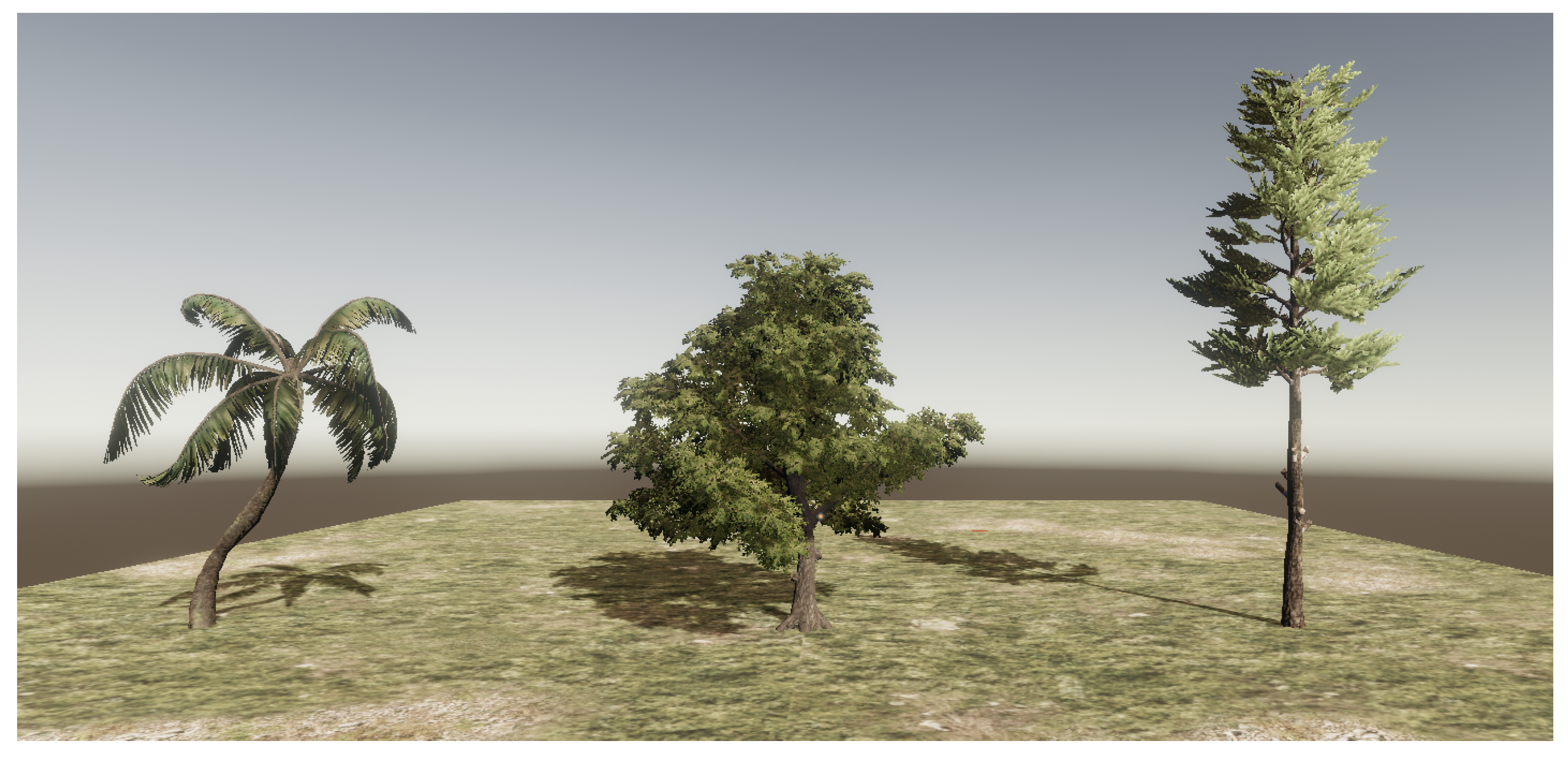
We develop a high realistic forest simulator to enable controlled experimentation of survey missions. It is based on the Unity graphics engine [30], which is a multi-platform framework and includes a terrain generation module based on a user-supplied height map, including ground textures and objects such as trees (either manually or randomly placed). Figure 1 shows the three different tree models included in Unity. Each tree can be customized by changing its size, color, and orientation. Including custom tree models, modifying the scene lighting as well as setting the camera parameters are also possible.
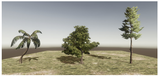
Figure 1.
Three different types of tree used in the simulation, from left to right: palm trees, planifolia, and conifers.
A series of image acquisition poses are generated to simulate a survey mission, following a predefined flight path, which involves setting the camera altitude, and angle. The poses are generated using the desired frontal and lateral overlap parameters, just as during a real survey planning. For each position, a simulated camera is placed in the appropriate location and an image is acquired.
For the simulation of a GPS sensor, the center of the environment is geo-referenced by a given coordinate system (typically UTM). In this way, the pose of all acquired images will be in reference to the scene coordinate system. Finally, these poses are perturbed using random white noise. The simulator also supports ground control points, by manually placing markers on the ground as done in real-world survey missions.
After acquisition is complete, the simulator generates an image sequence where the GPS poses are recorded in the EXIF label. This allows the same reconstruction process to be followed as would be done for images acquired with a real camera on a real survey mission.
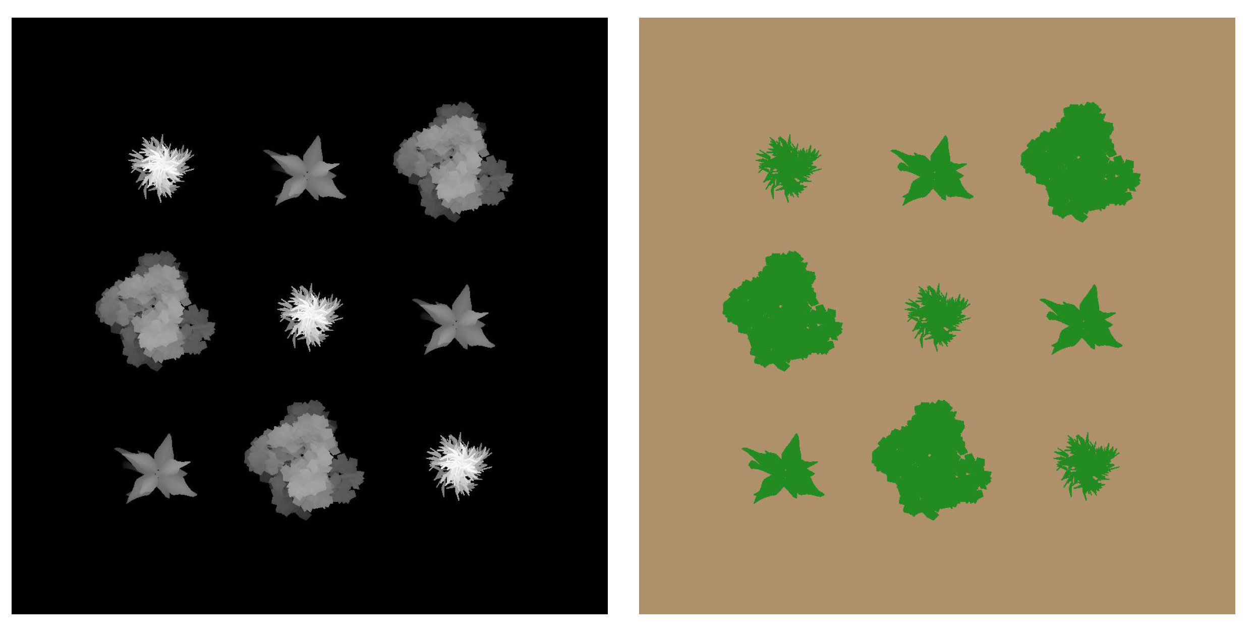
As ground-truth information, the simulator also generates the terrain mesh (as a point cloud), the CHM and a segmentation of ground and non-ground points in this map (see Figure 2). The simulator can also be used to report the crown size and highest point of individual trees.
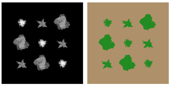
Figure 2.
Exported information from the simulator. The left image shows the height maps and the right image shows a segmentation of trees and floor for the Simple Trees Scenario.
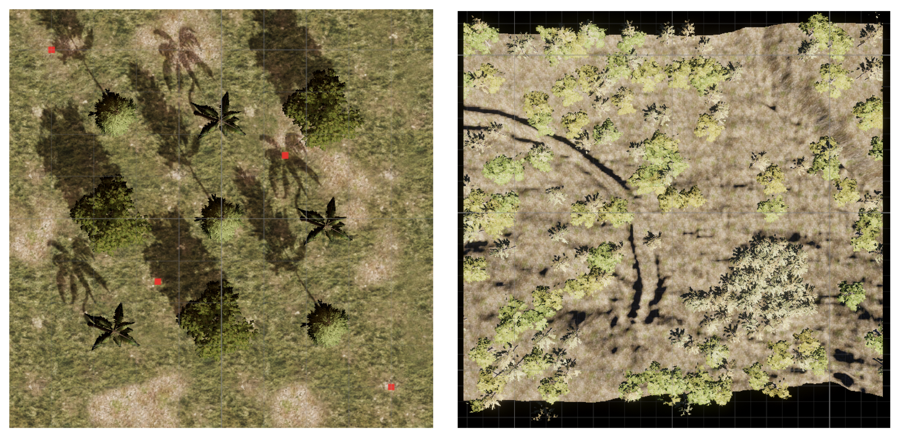
Two different scenarios were considered: Simple Trees (Figure 3, left) and Yosemite (Figure 3, right). The first scenario contains just nine trees of three different types spread over a square shaped region with flat terrain (see Figure 2). The second scenario aims to be a realistic representation of Yosemite National Park [31] by means of a real DTM obtained from LiDAR. Different tree types were randomly placed, followed by manual filling in some areas. Thus, the scenario results in a mix of both dense and sparsely forested areas.
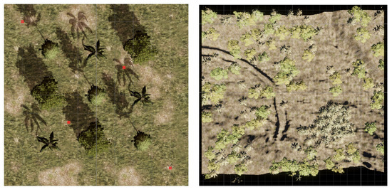
Figure 3.
Both synthetic scenarios used in this work: Simple Trees on the (left) and Yosemite on the (right).
In this way, we are able to simulate survey missions with different settings over synthetic scenarios in which the position of each tree (and each leaf) is perfectly known.
2.2. Survey Mission Settings
We characterize two different types of survey mission settings regarding sensor and flight, and consider four metrics to evaluate the resulting reconstruction: flight time, image processing time, point cloud precision and ground-sample distance (GSD).
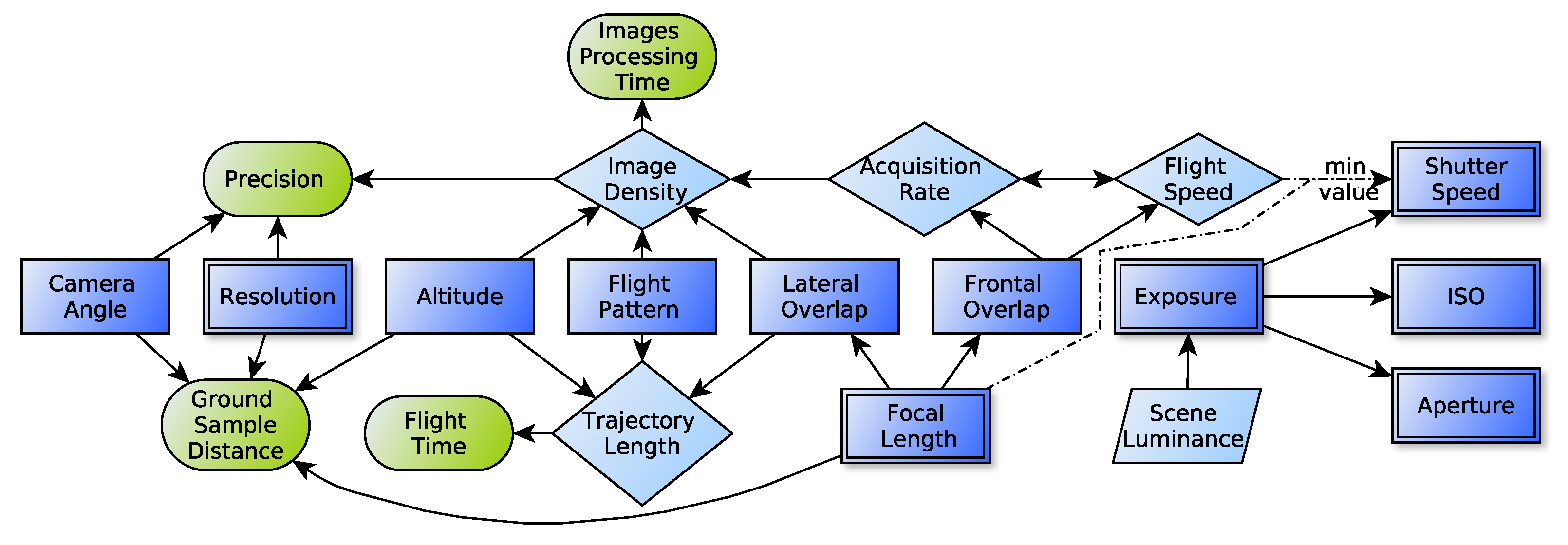
Since these variables are related in non-trivial ways, we present an analysis of these relations. Figure 4 outlines the relations between camera parameters and the rest of the survey settings and reconstruction metrics: arrows represent one parameter impacting in the value of another one, round nodes represent the four mentioned metrics.
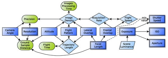
Figure 4.
This simplified scheme shows the relations between the settable (rectangles) and the control (rounded nodes) parameters for the aerial photogrammetry in forests. Square nodes denote user settable parameters (simple rectangles represent flight-related parameters while double border rectangles correspond to sensor related parameter), round nodes denote evaluation metrics, rhombuses denote inferred parameters, and slanted rectangles denote non-controllable parameters. The continuous arrows denote that the node affects the final value, while the dash arrows represent a minor limit.
We can further distinguish between user settings (those that must be explicitly chosen before the mission) and inferred settings (those indirectly affected by user settings). Flight-related user settings are image overlap (%), flight altitude (m), flight speed (), flight pattern (single or double grid) and camera angle (). Sensor related settings are: image resolution (Mpx), focal length (mm), sensor sensitivity (ISO speed), shutter speed (ms), and aperture (f number). The inferred parameters in our model are: image acquisition rate (Hz), image density (), and trajectory length (m). From these two groups is possible to estimate the value of the control parameters group: precision (m), image processing time (h), ground sample distance (cm/px), and flight time (s). These last groups will be used to evaluate the reconstruction process. Finally, we can also identify some variables that are not under user control whatsoever: scene luminance and maximum acquisition rate.
In general, there is no single configuration that guarantees a good reconstruction. To find the optimal parameter configuration, it is necessary to understand and quantify their effects. In the following sections we describe these variables and metrics in greater detail, discuss how they are related between each other, and give some hints towards good starting points for configuring values.
To evaluate the impact of the survey mission settings described below we used the simulated scenario Simple Trees and processed the resulting images using ODM. For each configuration we repeated the cloud generation process three times and then we estimated the mean of three relevant parameters: (1) distance between centers of bounding box (BB) of the original and generated cloud, (2) points number, and (3) BB size. We also used these parameters to detect wrong reconstruction when some thresholds are reached. In particular, if the BB was bigger than 100 m in any direction, or the BB was 150% bigger or 50% smaller than expected, the reconstruction was rejected.
2.2.1. Overlap
One of the most important mission settings is the image overlap: the percentage of the image that intersects with its neighbor image. The importance of this parameter lays in the fact that in order to create 3D geometry from images, at least two views of a portion of the surface are needed. Thus, the higher the image overlap, the greater the chance of establishing correspondences. Furthermore, correspondences are used to set restrictions to the underlying SfM optimization and thus a large number of these usually results in increased reconstruction accuracy.
Image overlap is directly proportional to the number of images per area: to achieve high overlap, more images are needed over the same distance, resulting in a denser distribution. This also implies that the image processing time will be higher. In other words, this parameter is a direct trade-off between reconstruction precision and efficiency. We can further distinguish frontal () and lateral overlap ():
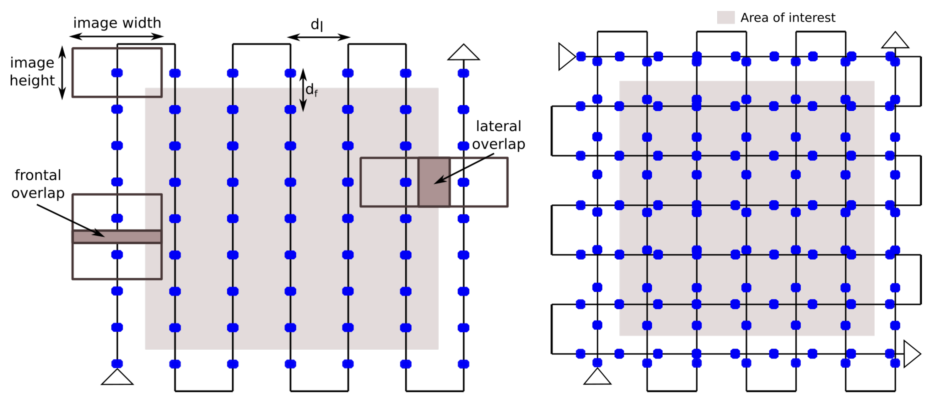
where is the (longitudinal) distance between consecutive pictures (m), is the (lateral) distance between flight lines (m) (see Figure 5), f is the focal length (mm), H is the distance from the camera sensor to the ground (m), w and h are the sensor width and height (mm), respectively.
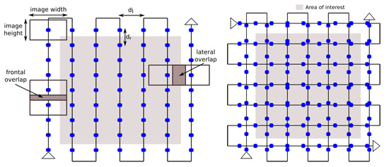
Figure 5.
Two flight mission plans, in the left a simple grid and in the right a double grid plan. Blue dots represent the places were pictures are planned to be captured. Frontal and lateral overlap are also shown.
Frontal overlap depends on the image acquisition rate, since higher implies that a greater number of images are acquired during the same time interval (assuming the flight speed remains constant). Thus, the combination of sensor capabilities and minimum flight speed will usually impose a higher bound on . Increasing lateral overlap will reduce . This means that a larger number of passes will be needed to achieve a tighter grid. The longer flight trajectory will result in higher flight time required (again, assuming constant flight speed). In conclusion, increasing will bear the same benefits of larger value but at the expense of longer survey missions, which will usually be limited by the flight autonomy of the UAS.
An alternative approach to increase , which does not impose a higher acquisition rate is to modify the flight pattern from a simple to a double grid (see Figure 5). This, of course, also negatively impacts flight time. For very irregular surfaces, such as the case of forest canopy, a high image overlap of at least is usually recommended. As a rule of thumb, each point should be visible in at least 4 to 5 images [7]. In this work, we tested values between and of both lateral and frontal overlap.
2.2.2. Flight Altitude
Flight altitude is also a trade-off between flight time and the reconstruction precision. If the image overlap is fixed, flying at a higher altitude will allow higher and . In other words, images will be taken further apart in time and space. Furthermore, as is increased, the flight trajectory will be shorter (less passes are needed) and flight time will be reduced. However, this all comes at the expense of reduced GSD (each pixel will represent a larger ground area) and point-cloud precision (image correspondences will be less accurately established).
Again, for the case of forestry applications, a relatively low altitude (relative to canopy) is recommended to maintain sufficient reconstruction detail. If this is not possible for the complete area, surveys performed at different flight altitudes may be combined in a single reconstruction. In this work, we evaluated different flight altitudes between 50 m and 200 m.
2.2.3. Flight Pattern
The flight pattern determines the path that the UAV will follow. For forestry applications the most used are simple or double grid in a squared or rectangular area (see Figure 5). Simple grid is less time consuming, but double grid is more accurate since it has more images and from different sides. Thus, depending on the application it will be adequate to use one or the other. When generation of 2D maps is the main interest, the terrain is mostly flat or the area to be surveyed is large, the simple grid is usually used. For 3D models or when the terrain has height variations (buildings, rugged terrains such as precipices) and the area to be surveyed is small the double grid will give better results. In general, in order to improve the 3D models generation the flight pattern includes a combination of different camera angles (in general nadir and another value) and sometimes even different flight altitudes. In this work, we tested both single and double grid patterns combining with different altitudes and camera angles.
2.2.4. Camera Angle
Camera angle is the tilt angle of the camera with respect to the ground, for example a camera pointing down corresponds to 90, while a camera pointing forward to 0. Camera angle is an important parameter in the mission setting as adding oblique images allows observing new parts of the environment, such as the side of trees, generating richer reconstructions. However, if the angle is too low, it may be difficult to match the images, as the area shared between them could be reduced due to occlusion. In addition, if the horizon is observed, it will give a wrong reconstruction or directly an error in the SfM process, as the system will try to include this faraway areas in the reconstruction. In this work, we tested four angle values between 60 and 90, using both a simple and double grid flight pattern.
2.3. Ground Sample Distance
The ground sample distance (GSD) is related to the detail obtained during the reconstruction in terms of the area represented by each image pixel:
where w is the sensor width (mm), H is the flight height, f the focal length (mm), is the image width (pixels), and is the angle between the nadir direction and the sensor line-of-sight. The factor only has an effect when the camera direction is not nadir [32].
2.4. Reconstruction Error
To measure the reconstruction error we compare the obtained reconstructed surface with a reference mesh. Since we use a simulator to generate reference meshes in our reconstruction experiments, the ground-truth mesh is readily available. For real-world missions, this could also be performed if a terrestrial laser scan is available (this is not usually the case) or by means of a surface reconstructions process, such as Poisson Surface Reconstruction [33], which is prone to smooth out details and extrapolation errors. For this reason, in real-world survey missions reconstruction error is typically measured by means of comparing expected to estimated coordinates of hand-placed ground-control points.
Point Cloud Comparison
To evaluate the precision of a given simulated reconstruction we compare it with the ground truth mesh (densely sampled into a point cloud) exported from the simulator. To estimate the distance between two surfaces, we follow the definition of root mean square error (RMSE) from METRO [34]. First, we define the point-to-surface distance for a given point p and a surface mesh M, as the euclidean distance to the closest point in the sampled mesh M.
where d is the euclidean distance between two points.
We can now define the root mean square error () between two surfaces and as:
We should note that, the number of points in the ground truth mesh are always the same in each experiment and the surfaces to compare with are aligned, allowing us to use the RMSE as a metric to evaluate the 3D reconstruction quality w.r.t. .
It is worth mentioning that is not always equal to since the closest point in may have a different closest point in . In the following, we will note and for and , respectively.
In particular, is typically used in the literature [35,36] where the reference mesh corresponds to another reconstruction of the same area. Instead, in this work, is a very detailed ground-truth surface mesh exported by our simulator while is a point cloud obtained by our reconstruction method. This means that will be a subset of , since may have holes and missing data (such as tree trunks, in forest mapping) due to occlusion. As a result, will usually be higher when there is data missing in the reference mesh, while will not be affected by this issue. On the other hand, this means that itself is not enough as an indicator for the reconstruction quality, since we not only care about the precision of the obtained surface but also about the approximation of the ground truth surface.
Thus, in this work we choose to present both and , since the latter will give a measure of the precision of the points in while the former will indicate how well the whole reference surface was approximated.
2.5. Digital Terrain Model Generation
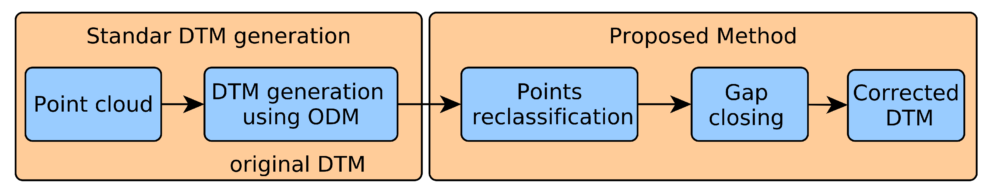
The DTM describing all ground points in the environment is a key input to estimate canopy height and other forest structural parameters. In this section we propose a novel method to generate accurate DTM using only the point cloud. The workflow for this computation is outlined in Figure 6. First, we perform an initial classification based on the Simple Morphological Filter (implemented in the ODM tool) [19], which assigns each point to either ground or non-ground class. To improve on this initial result, we then compute the best-fitting plane for all ground points and then reclassify all points by considering their distance to the plane. Finally, to close gaps in the ground point cloud, we also estimate a plane for each gap and generate points uniformly over this surface. The SMRF [19] algorithm used by ODM to classify the cloud points utilize four parameters: slope (slope rise over run), window (max window size), elevation threshold, and scalar (elevation constants used to classified the cloud points as ground or not ground). ODM by default uses parameter settings which are not ideally suitable for forest reconstructions. In [19], an optimized parameter set is proposed for an area with low altitude and dense vegetation. Thus, for these experiments we tried both the default and optimized parameters, as well as up to 80 random combinations. To evaluate the results, we compared the final ground map to the ground truth, obtained from the simulator.
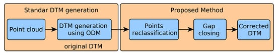
Figure 6.
Workflow scheme for the digital terrain model generation using the proposed method.
The DTM is then constructed with the PDAL Library [37] using as input all ground points. After this, the CHM can finally be obtained by subtracting the height of the ground at each location to the z coordinate of every non-ground point in the DSM. The DSM is calculated similarly to the DTM, but by using all the cloud points.
In the following sections, we describe the point-cloud re-classification and gap closing in more detail because they are the key steps of the method to obtain accurate DTM.
2.5.1. Points Reclassification
From the already classified ground cloud, we first partition the points using only their X and Y coordinates (see below). Then, for each partition, we estimate the best-fitting plane using a RANSAC (Random sample consensus) scheme for robustness to outliers. Finally, we reclassify all points above the plane by some distance threshold as not ground and all points closer as ground. The pseudo-code for this step is presented in Algorithm 1.
| Algorithm 1 Reclassification of Ground Points |
|
To partition the cloud points, we considered four alternatives: (i) Plane, which considers the entire cloud as a single partition and use only one plane to adjust it; (ii) Uniform Division, an iterative method that divides the cloud in four uniform sections, and continues recursively until either the area covered by each subdivision or the number of points contained in it are below a given threshold; (iii) Median Division, similar to the uniform division, but considering the median of the points number in each area instead. The main idea is to have partitions with the same points number, and (iv) Surrounded, which attempts to find good planes in the areas without points (generally corresponding to dense tree areas), using the border of them to estimate the best plane. The first step is to find all the areas without points, and create a partition for each one containing all the surrounded points. After this, all the remaining points of the cloud are assigned to the same partition.
2.5.2. Gap Closing
To fill all gaps remaining in the point cloud of ground points, we apply a gap closing algorithm. We follow a similar approach as for reclassification by closing each gap by means of a plane. From the ground points of the reclassified cloud, and using the surrounded method we separate the cloud in several partitions. Each gap has associated one partition, and using RANSAC we estimate the best plane for each one. After this, equidistant points are generated over the plane and added to the ground cloud. Algorithm 2 describes this step of the method.
| Algorithm 2 Ground Extension |
|
2.6. Structural Parameter Estimation from SfM
In this work we focus on two main forest structural parameters than can be obtained using SfM techniques: tree coverage and height. While computing tree height can be generalized to obtaining the CHM, tree coverage can be estimated by the ratio of forested to total area:
where is obtained directly from regions of the CHM with non-zero height (considering a threshold). While the CHM could be used to obtain individual tree height, it is generally more useful to a height based segmentation of the CHM, considering that forested areas usually show sectors with markedly distinct height (due to different successional stage, dominant species, soil condition, or management).
2.7. Selective Logging Detection
Selective logging detection results from comparing reconstruction of the same surveyed area at different times. First, the CHM corresponding to each survey is computed as explained in previous sections. The ground-referenced point clouds are then aligned and the difference is computed, using the oldest as a reference. Algorithm 3 describes the procedure.
| Algorithm 3 Changes Detection |
|
The first step is to use the correction in the ground estimation described previously with the function CorrectGroundEst for both clouds, to then align them using AlignClouds. After this, both CHM maps are generated with the CHM function, to then calculate the difference between them. The function BinClasChange uses a threshold to classify every point as changed or not. This threshold is defined as a third of the altitude of the highest point since this value exceeds the noise and at the same time detects changes in the trees; however, the user can change it manually. The function MorphFilter applies two morphological filters (first erosion and then dilatation) in order to eliminate noise, and the same filters in the inverse order, to eliminate little holds in the big forested areas. Finally, the contours are calculated with Contours and then a minimal area filter is used to eliminate small areas with MinAreaFilter.
2.8. Fieldwork
Finally, we performed a series of real-world experiments both for the ground segmentation step and structural parameters estimation. These experiments where carried out in forested environments located in different protected areas in Argentina and using different UAVs. In Nahuel Huapi National Park (Neuquén Province) an area of 200 × 200 m was surveyed using an DJI Mavic 2 Pro UAV. In Ciudad Universitaria-Costanera Norte Ecological Reserve in Buenos Aires City, we used a DJI Phantom III Standard to make a 3D model in an area of around 20 hectares. In Ciervo de los Pantanos National Park (Buenos Aires Province) we used a custom built fixed-wing aerial platform based on the commercial Skywalker 1900 fuselage.
3. Results and Discussion
The first set of experiments are focused on establishing certain aspects regarding the survey mission setup with a simulator as described in Section 3.1. The second set of experiments are aimed towards experimental validation of the DTM generation method, presented in Section 3.2. Third, forest structural parameters estimation is presented in Section 3.3. Finally, selective logging detection process using the proposed DTM generation method is also validated Section 3.4.
3.1. Survey Mission Settings Analysis
In this section we evaluated the impact of some of the main survey mission settings over the SfM reconstruction process. For this experiment we used the simulated scenario Simple Trees and processed the resulting images using ODM. In all the cases we set: image resolution 4000 × 3000 px, focal distance 3.61 mm, sensor width 6.24 mm, and sensor height 4.68 mm. The default values were: flight altitude 100 m, camera angle of 90, and a GSD of 4.32 cm/px (this value will change with flight altitude and camera angle according to (3), unless another value is specified.
3.1.1. Overlap
As previously mentioned, image overlap is strongly related to reconstruction quality since it mostly determines the number of correspondences that can be established between adjacent images (the higher the overlap, the higher the matches). We initially tested values between and of both lateral and frontal overlap to determine a usable range of values. We then focused on overlap values in the range between between and , considering also that values are usually recommended for SfM reconstruction of forests. Results of these experiments are presented in Table 1.

Table 1.
Quality metrics for different overlaps: N Img (number of images), N Points (number of points), FD (flight distance), (Root Mean Square Error) using the ground truth mesh as reference and using the reconstructed cloud as reference in the estimation of RMSE. In blue, is shown the best five results for each metric, and in dark gray a good option for the trade-off between precision and overlap is remark.
When analyzing the results of these experiments we can see a direct relation between image overlap and the number of images and, thus, the number of generated 3D points. Moreover, lateral overlap has greater impact over these variables since it results in a tighter flight path with more passes over the survey area.
Is interesting to note that and estimations have contradictory behaviors. For case, the error is in the order of the centimeters and it slowly grows with the overlap. On the other hand, abruptly decreases when increasing the overlap. To clarify this behavior, Figure 7 shows the reconstruction of two cases: F75%L75% and F95%L95%. For the case F75%L75% we have the lowest value of , but the reconstruction is lacking a large number of points, in particular in the trees. On the other hand, for this case has the highest value since there are several areas without points, and this increases the estimated error. The case F95%L95% shows a dense reconstruction as expected. It additionally represents one of the lowest values of , but a higher value of . As a conclusion, represents a valid metric to check that the estimated error of the reconstructed points is within the expected parameters, but it results are insufficient to evaluate the quality of the reconstruction. We will prioritize the value in order to evaluate the reconstruction parameters.
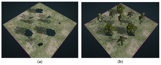
Figure 7.
Comparison between two reconstructions belonging to two different overlap flights (highest and lowest values of Table 1). Although in Table 1 the lowest value of is for the case F75%L75%, the reconstruction is lacking a large number of point in the trees. This example shows that is a good indicator of the points precision but is not good to evaluate the quality of the reconstructed cloud. (a) Reconstrution: F75% L75%. (b) Reconstrution: F95% L95%.
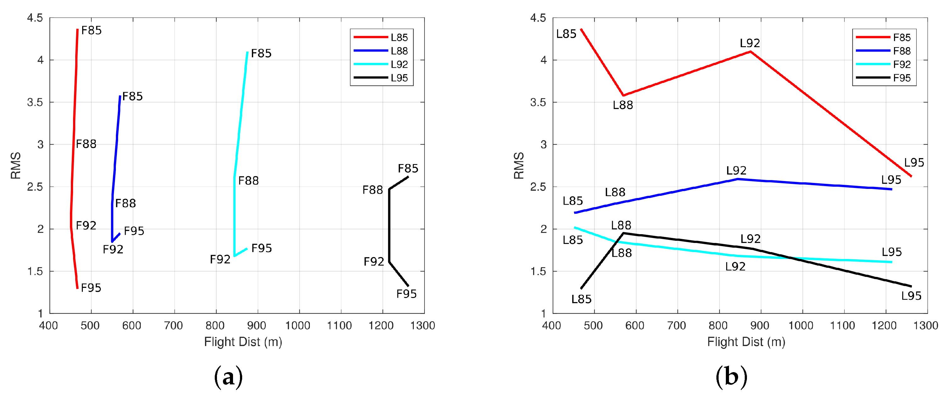
Following the value of , we found that as expected values of overlap lower than do not give usable results. We can also analyze the effect of varying either frontal or lateral overlap leaving the other parameter fixed (see Figure 8). We can see that when lateral overlap is increased and frontal overlap is left fixed, flight distance increases as previously mentioned. Conversely, when frontal overlap is increased and lateral overlap is left fixed, flight distance remains mostly constant. Finally, we can observe that precision mostly increases depending on frontal overlap, whereas increasing lateral overlap does not have a big impact of precision.
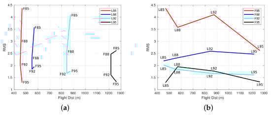
Figure 8.
Flight distance versus the error, for different values of frontal and lateral overlap. (a) Lateral overlap variation. (b) Frontal overlap variation.
From all of these combinations we found that using lateral overlap gives good results overall. In particular, combining this value with frontal overlap gives the best trade off in terms of accuracy and number of points/images and flight distance. These results are in line with previous analysis, in particular with those obtained in [24], where the authors also analyzed separately the effects of both forward and lateral overlap, although using a video footage.
3.1.2. Camera Angle and Flight Pattern
In this experiment we analyzed the effect of different camera angles on the reconstruction. We tested four angle values between 60° and 90°, using both a simple (see Table 2) and double grid (see Table 3), with a flight altitude of 100 m with a frontal and lateral overlap of and , respectively. We did not consider angles lower than 60° since in general too much sky would be visible in the pictures and this brings problems for the image processing pipeline.
Table 2.
Quality metrics for different camera angles: N Img (number of images), N Points (number of points) and RMSE (Root Mean Square Error). Blue values represent the best result.
Table 3.
Quality metrics for different camera angles in a double grid setup. Blue values represent the best result for each configuration.
When comparing single grid flights with different camera angles, the first thing to note is the increment of points in the clouds for bigger angles. This can be attributed to the fact that although for small angles the observed surface is greater, the overlap between images is reduced. Nevertheless, regarding reconstruction precision, we did not find significant differences when the camera angle changed.
For the double grid case (see Table 3) we repeated the experiment, considering that now the angle may change between either orientation of flight lines (thus we will name each angle and ). In general we can see a similar behavior than for a simple grid: higher angles lead to higher precision and more 3D points. Regarding reconstruction precision, for both overlap cases, the configuration and show the best results, especially for the lower image overlap case, where the number of 3D points is smaller. This result reinforces that obtained by [26,27], showing the relevance of incorporate oblique images to make 3D reconstructions in forest landscapes.
3.1.3. Flight Altitude
For the single grid case (Table 4), as expected, higher altitudes result in a smaller number of images and 3D points. This in turn shortens the flight distance but also reduces the precision.
Table 4.
Quality metrics for different altitudes for simple and double grid options with a frontal and lateral overlap of and , respectively. Blue values represent the best result for each configuration.
For the double grid case, we tested combinations of different altitudes for flight lines in each orientation (Table 5). In this case, while there is also a decrease in the number of images, 3D points, and flight distance as altitude increases, we can see that the precision not always decreases. In particular, the configuration corresponding to the best precision for this experiment was m and m.
Table 5.
Quality metrics for different altitudes for simple and double grid options with a frontal and lateral overlap of and , respectively.
3.2. DTM Generation and Ground Segmentation
We conducted a series of experiments to evaluate our DTM generation method and the ground segmentation required to ultimately obtain a CHM. To establish a baseline, we first performed a segmentation using ODM over the ground-truth point-cloud obtained from the simulator. We then attempted to improve this result by considering the different segmentation strategies.
3.2.1. ODM Classification
In the first instance, we compared different parameter settings in the ODM algorithm. Table 6 shows the results of default, optimized [19], and the best option among the 80 random combinations evaluated. We used the since, as we showed before, it gives better results, especially when the cloud that has to be compared has gaps.
Table 6.
RMSE error for different settings of the ODM ground segmentation. The optimized corresponds to the values recommended in [19]. Win stands for window and Th for threshold.
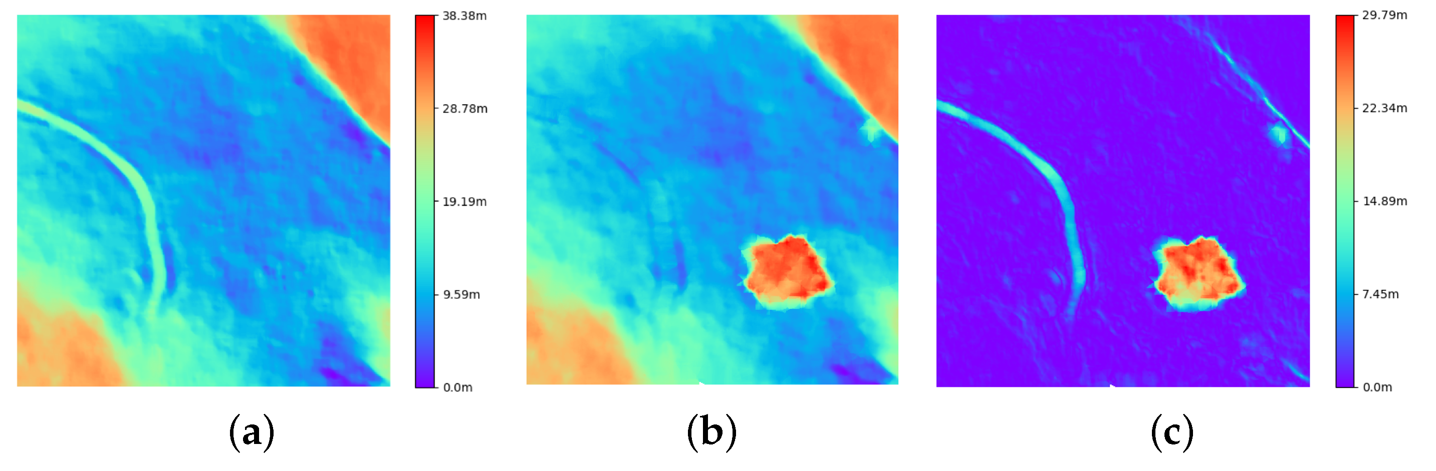
In Figure 9 we also compare the ground-truth DTM to the one obtained by the aforementioned ground classification method (with the best set of parameters). When observing the difference (Figure 9c) between ground-truth (Figure 9a) and estimated (Figure 9b), we can identify three areas with large errors, which correspond to an open ditch on the left, a large group of trees in the middle, and a small slope and a tree in the top right part.
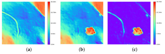
Figure 9.
The left and the middle show the DTM ground truth and the one obtained with the best set of parameters of Table 6, respectively. The right shows the error (calculated as the difference between the other two maps) in the DTM estimation. (a) Ground-truth DTM. (b) Estimated DTM. (c) Difference.
3.2.2. Point Reclassification
In this section we evaluate the improvement of our point reclassification method over the initial result obtained directly from ODM. We tested the four cloud segmentation strategies, described in Section 2.5.1. In Figure 10 we show the partitions generated as a result of applying each strategy. The reclassification process is then performed in each partition and the final DTM is generated.
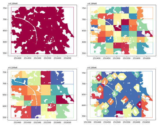
Figure 10.
Partition used in ground points reclassification: (top left) One Plane, (top right) Uniform, (bottom left) Median and (bottom right) Surrounding.
The median method present the best results since it eliminates the wrong classified area corresponding to the dense trees, without affecting the rest of the scenario. Nevertheless, none of the methods show improvement related with the other two areas of error (the open ditch on the left and the slope on the right). The method of one plane also removed these points, but since only one plane was used and the terrain was not flat, the corners were wrongly classified as not ground, because the difference with the plane was too big. Something similar happened with the surrounded method, since it also uses one plane for all the terrain. Finally, the uniform method was not able to remove the point of the dense tree area, since this area was too large and different partitions were set, making it impossible to estimate a good plane.
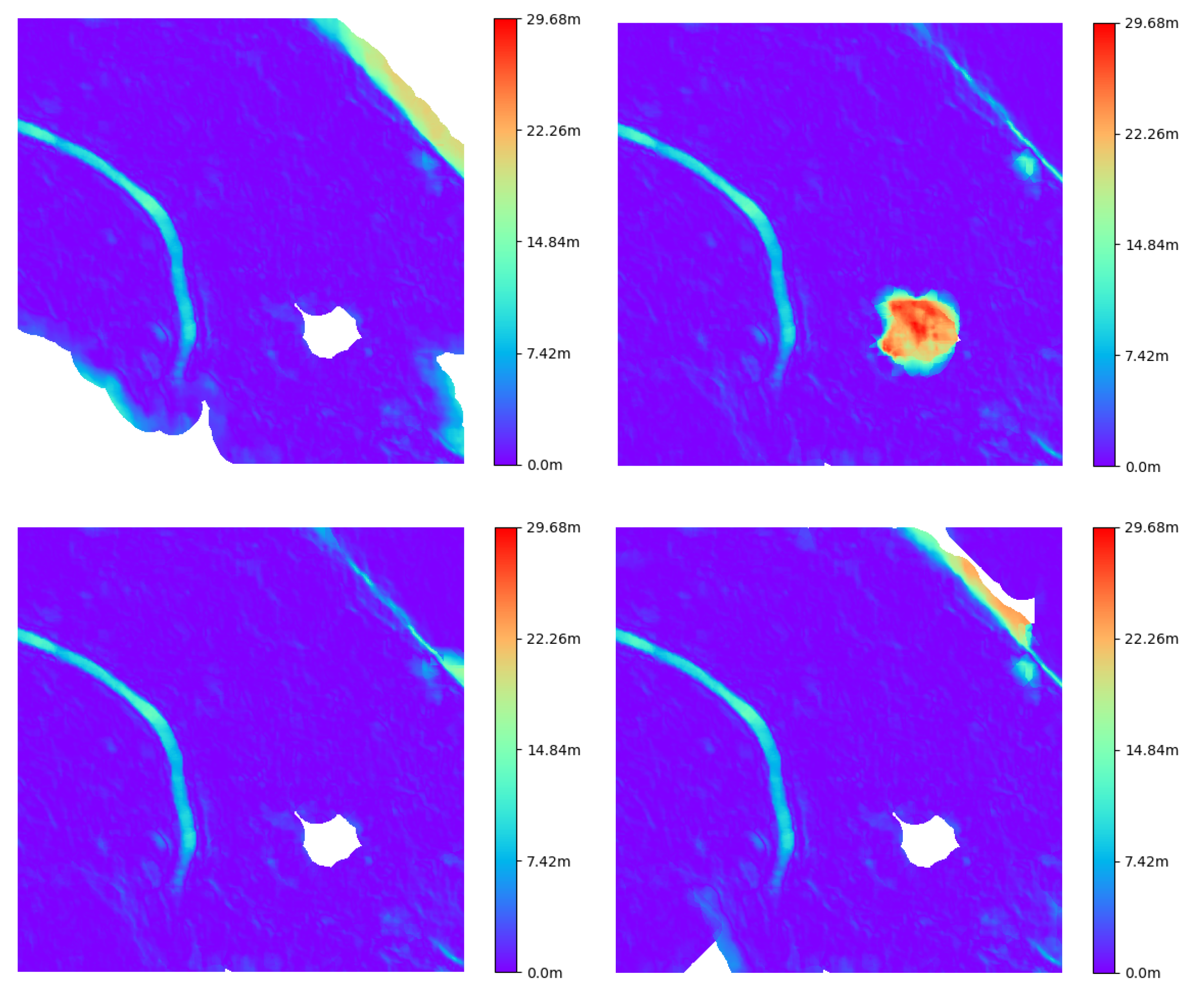
From each DTM we measure the error as in the previous section (Figure 11). White areas correspond to zones that were reclassified as not ground, and the interpolation of ODM cannot fulfill those areas. It is desired to have them in the wrong classified areas in the original DTM, but not in well classified zones. This areas will be fulfilled again in the ground extension process.

Figure 11.
DTMs errors after reclassified as not ground some points (white areas) using the proposed methods: (top left) One Plane, (top right) Uniform, (bottom left) Median and (bottom right) Surrounding.
Using Metro we compared these DTM estimation with the ground truth, and the results are shown in Table 7. Again, median partitioning method has the best performance.
Table 7.
Comparison, using METRO, between the different partitioning methods and the original mesh. Cov % is the coverage percentage of the original model. The Median method shows the better performance in all the metrics.
3.2.3. Ground Extension
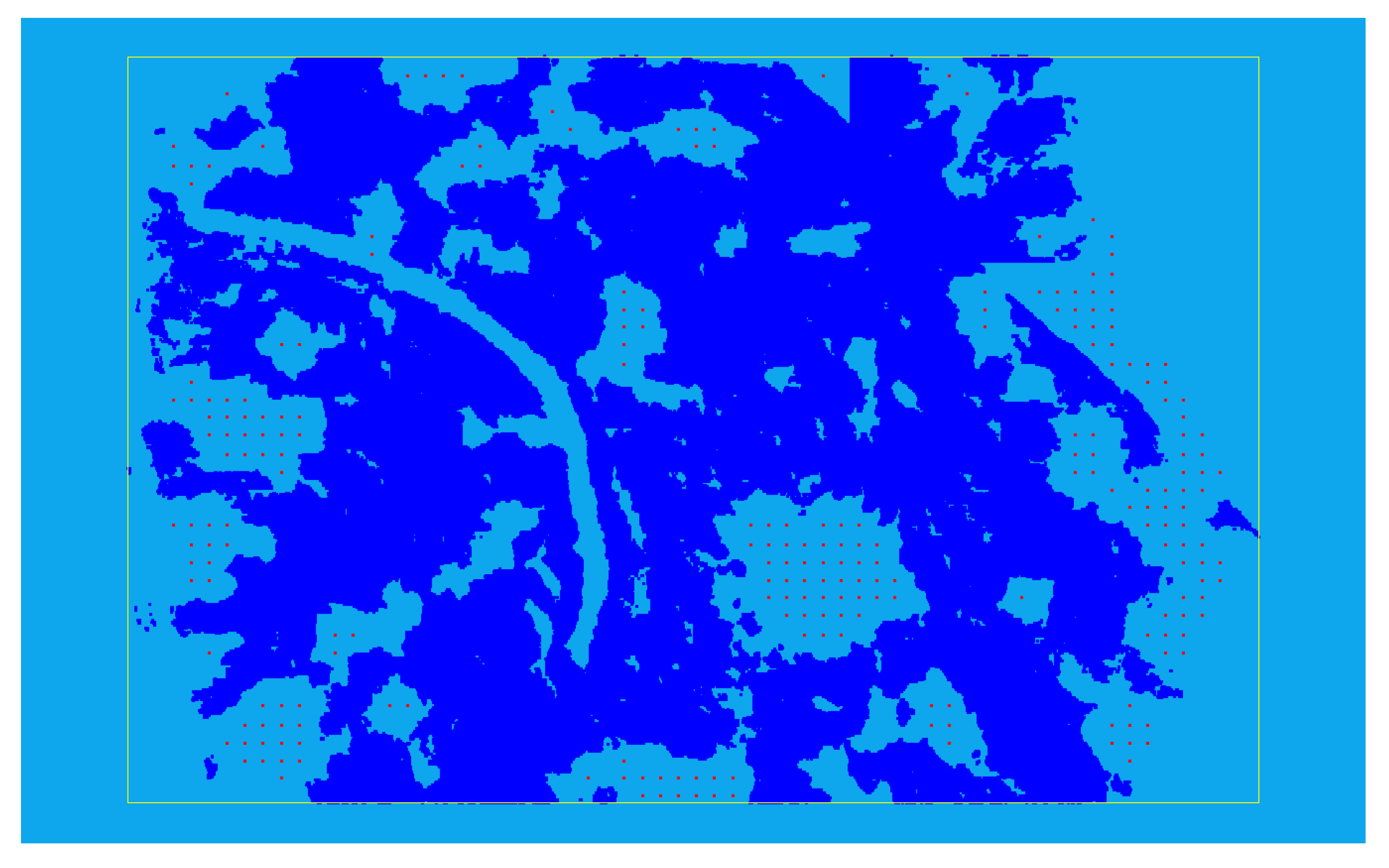
For each of the reclassification results obtained in the previous section, we then applied the ground extension method proposed in Section 2.5.2. As an example, in Figure 12 we show how points are added in gaps for one of these cases.
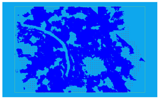
Figure 12.
Added points (red) in the cloud for a distance of 5 m.
In Table 8 we show the new results after applying the ground extension step. Observing these results, we realize that the Surrounded method shows the best performance.
Table 8.
Comparison, using METRO, between the different partitioning methods and the original mesh. The Surrounded method shows the better performance in all the metrics, and shows a bigger improvement in comparison with the default method used by ODM.
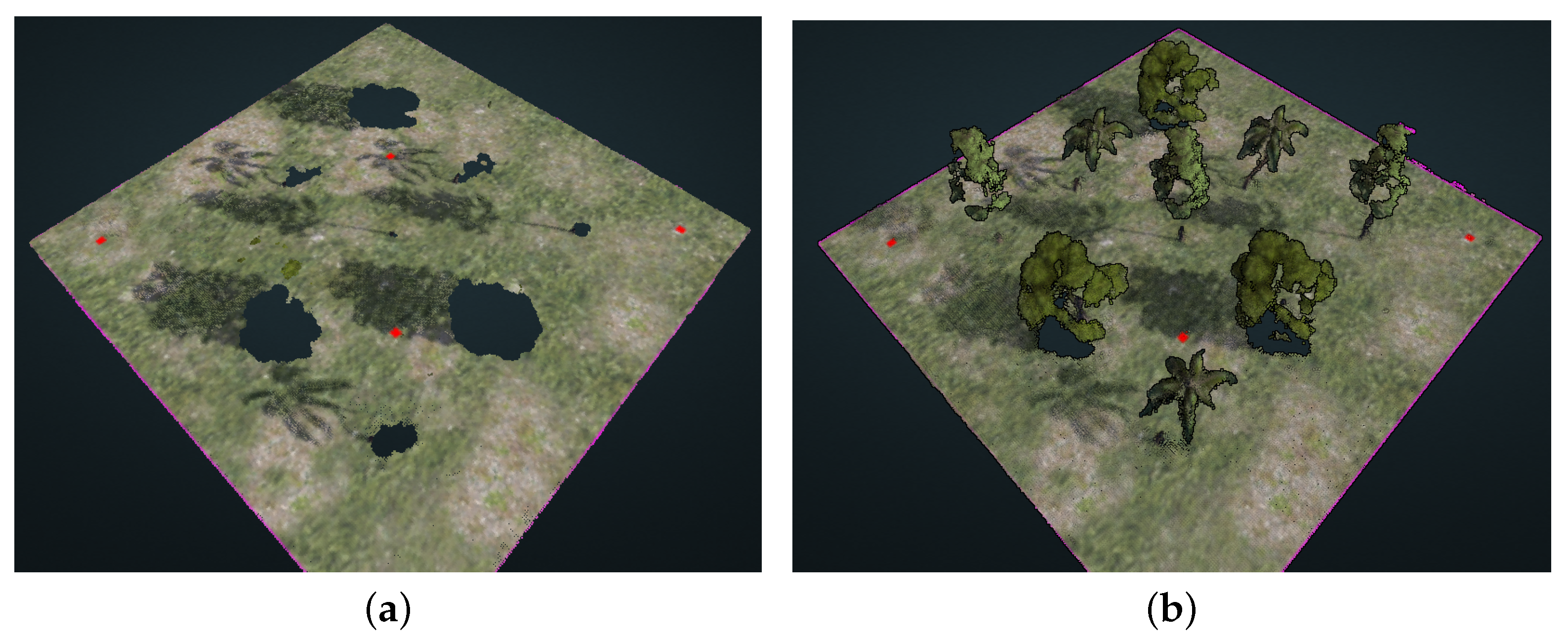
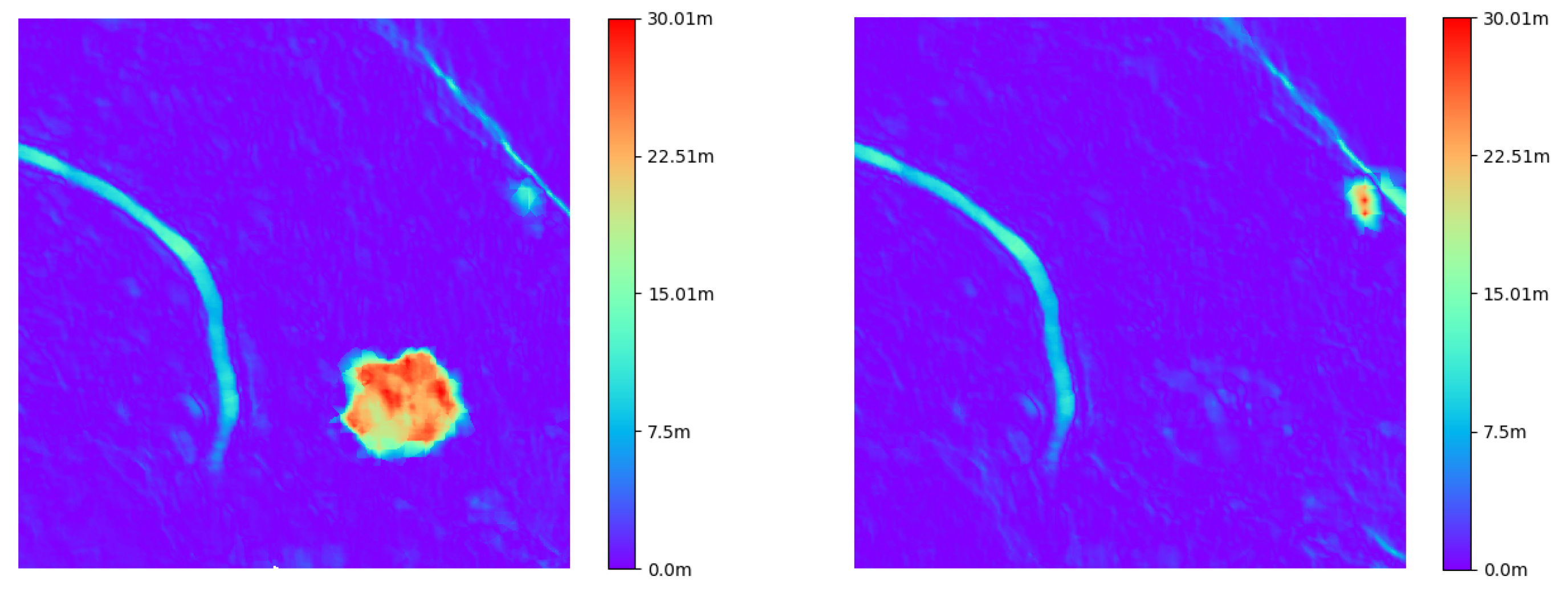
Finally, in Figure 13 we compare the final DTM obtained via ODM and the improved one after applying the reclassification and ground extension methods with the surrounded strategy. We can here see that our approach considerably improves the result, which corresponds to an RMSE improvement from 4.287 to 1.843.

Figure 13.
Differences within the original method used for ODM (left), and our proposed method (right) to estimate the ground.
3.2.4. DTM in Real-World Cases
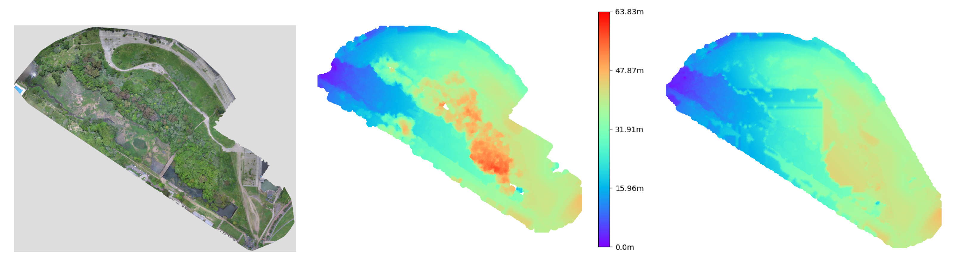
For the study area in Nahuel Huapi National Park, the resulting orthomosaic is presented in Figure 14a and the DTM obtained via ODM with the default configuration is presented in Figure 14b. We can observe that on the right of the image there are some trees (red areas) that were classified as ground and that there are also gaps (white areas) in the map. These issues occur since most of the surface is covered by trees and the default classification method is unable to correctly detect the ground. Both of these problems are solved when using the Algorithm 2 (see Figure 14c), were a mostly flat terrain is detected.
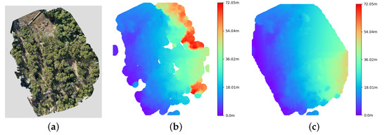
Figure 14.
Original orthomosaic of the relevated area (left), DTM with the Default algorithm of ODM (middle) and DTM corrected with our method. (a) Orthomosaic. (b) Default. (c) Proposed Method.
Figure 15 shows the results obtained for Ciudad Universitaria-Costanera Norte Ecological Reserve. The orthomosaic is on the left side, where it is possible to observe this area. The middle image correspond to the default DTM, where again some of the trees are wrongly classified as ground and also there are some gaps. When running Algorithm 2 (right) with the same parameters as in the other reconstructions, the gaps are well estimated and disappear. Nevertheless, some areas are wrongly fulfilled, assuming a flat terrain during the ground extension. This can be easily corrected by delimiting the border of the reconstruction.
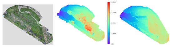
Figure 15.
Original orthomosaic of the relevated area (left), DTM estimated with the Default algorithm of ODM (middle) and DTM corrected with our method (right).
3.3. Structural Parameters
In this section we present our results when estimating the structural parameters of interest: tree coverage and canopy height.
3.3.1. Coverage
Once ground segmentation is performed, estimating tree coverage is trivial since it reduces computing the percentage of pixels classified as ground with respect to the total area in question. We can use the Yosemite simulated scenario again to compare tree coverage results to ground-truth information. When using ODM, the resulting coverage is . With our approach, coverage is . Compared to the ground-truth value of we can indeed observe our method results in an improvement. This measurement shows the importance of precise ground segmentation as it directly impacts coverage computation. Figure 16 shows the tree segmentations obtained for each method and the difference to ground truth segmentation.
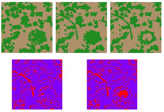
Figure 16.
(Top left): Expected segmentation from the real mesh. (Top middle): segmentation using the ground estimation correction. (Top right): segmentation with the default ground estimation. (Bottom): difference between the expected segmentation and, at (left), the one with the ground estimation correction and at (right), with the default estimation.
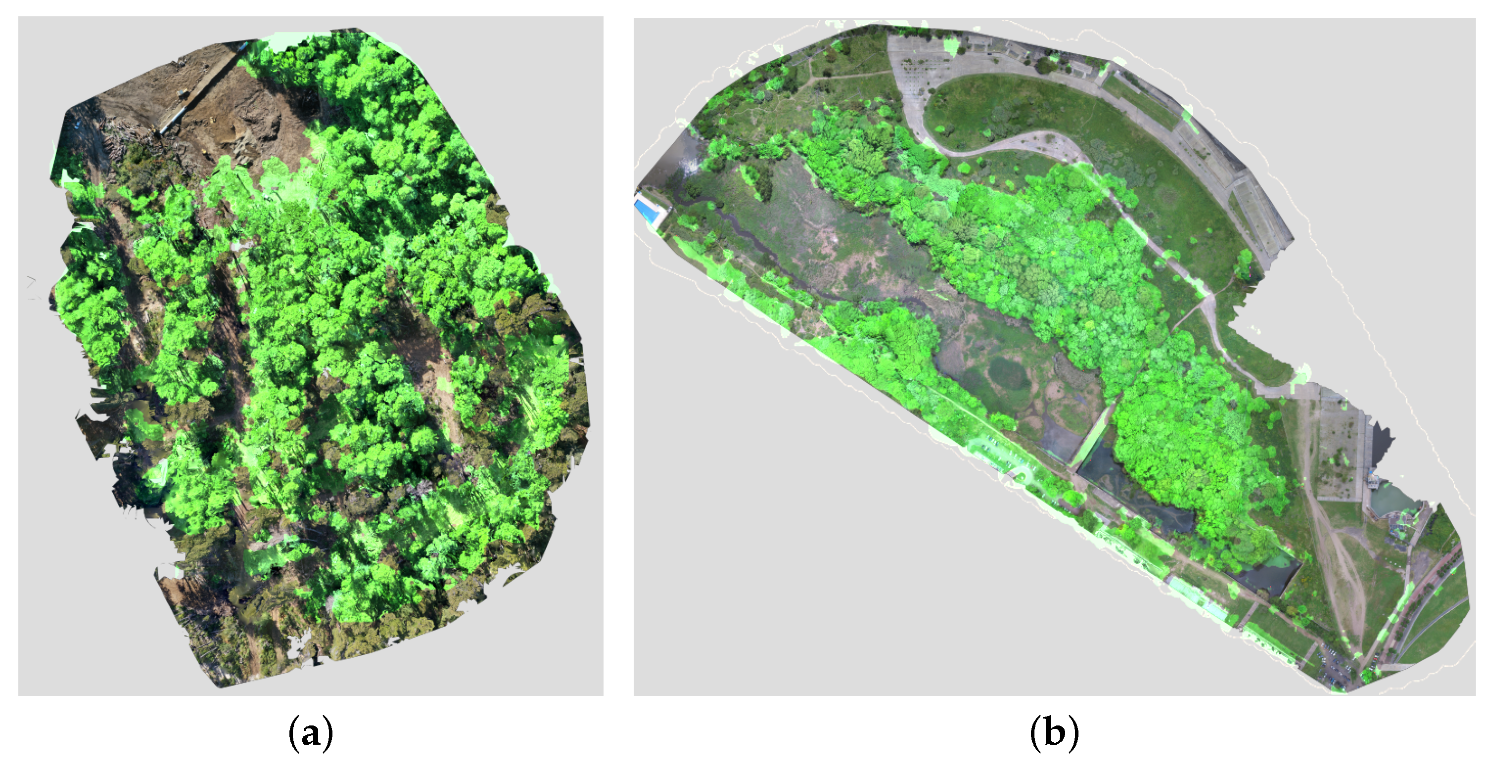
On the other hand, we also computed tree coverage for real-world experiments. Since in this case we do not have ground-truth information, only qualitative analysis is performed. In Figure 17 we overlay the segmentation result over the orthomosaics of Villa La Angostura and Reserva Ecológica Costanera Norte (RECN) experiments. In general we can observe that most of the forested areas are correctly classified as not ground. The coverage percentage for Villa La Angostura is estimated as and for RECN.

Figure 17.
Overlay between orthomosaci and the areas covered by trees (fluor green) for the Villa La Angostura and RECN experiments. (a) VLA. (b) RECN.
3.3.2. Tree Height
A second result we can obtain from the CHM is tree height. As previously mentioned, as detecting individual trees is not really feasible for very densily forested areas, we can resort to obtain a height segmentation from the CHM for the purpose of isolating potentially different forest types.
In Figure 18 we show the regions with similar tree height for a reconstruction of the Ciervo de los Pantanos national park. To build this segmentation map we extended ODM software to allow specifying different height intervals to be mapped to a class (based on knowledge of available forest types in the area).

Figure 18.
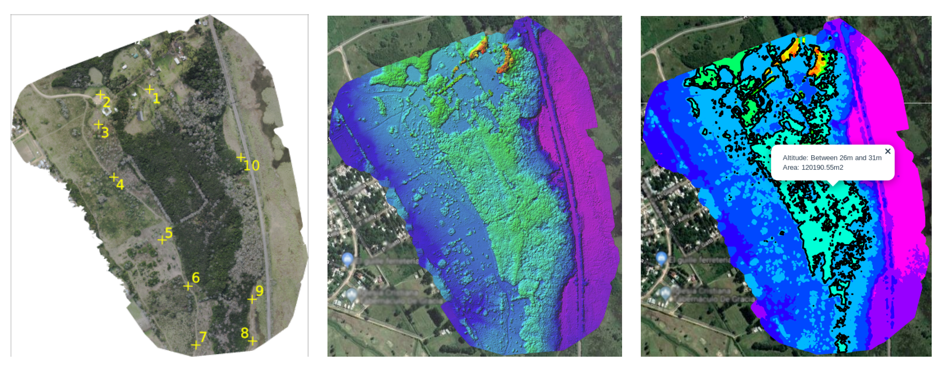
National Park Ciervo de los Pantanos. (Left): Orthomosaic generated, where yellow marks represents the CGPs. (Medium): corresponding height map. (Right): segmentation stratified by heights.
3.4. Selective Logging Detection
In this section we evaluate the ability of our system to detect changes between two survey missions of the same area at different times. In the context of forestry, this feature has multiple applications such as selective logging detection. We performed two sets of experiments: first in the Yosemite simulated environment and then on a real-world scenario of a construction site inside a forested area.
3.4.1. Simulation
In this experiment we generated an initial tree population in the Yosemite simulated environment and then a second one with some of these trees removed from three different areas of the map. We performed two simulated survey missions and then attempted to detect the differences.
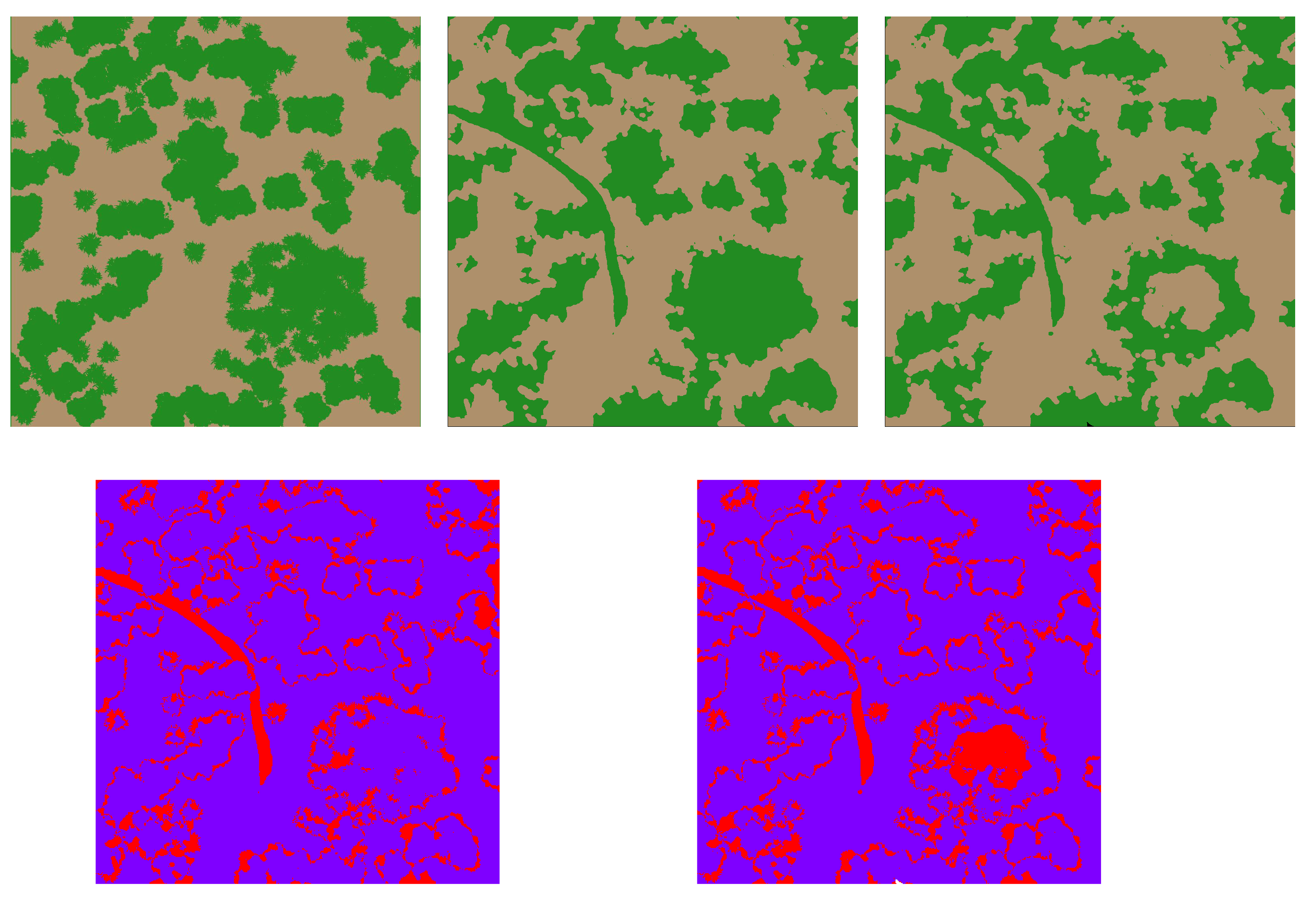
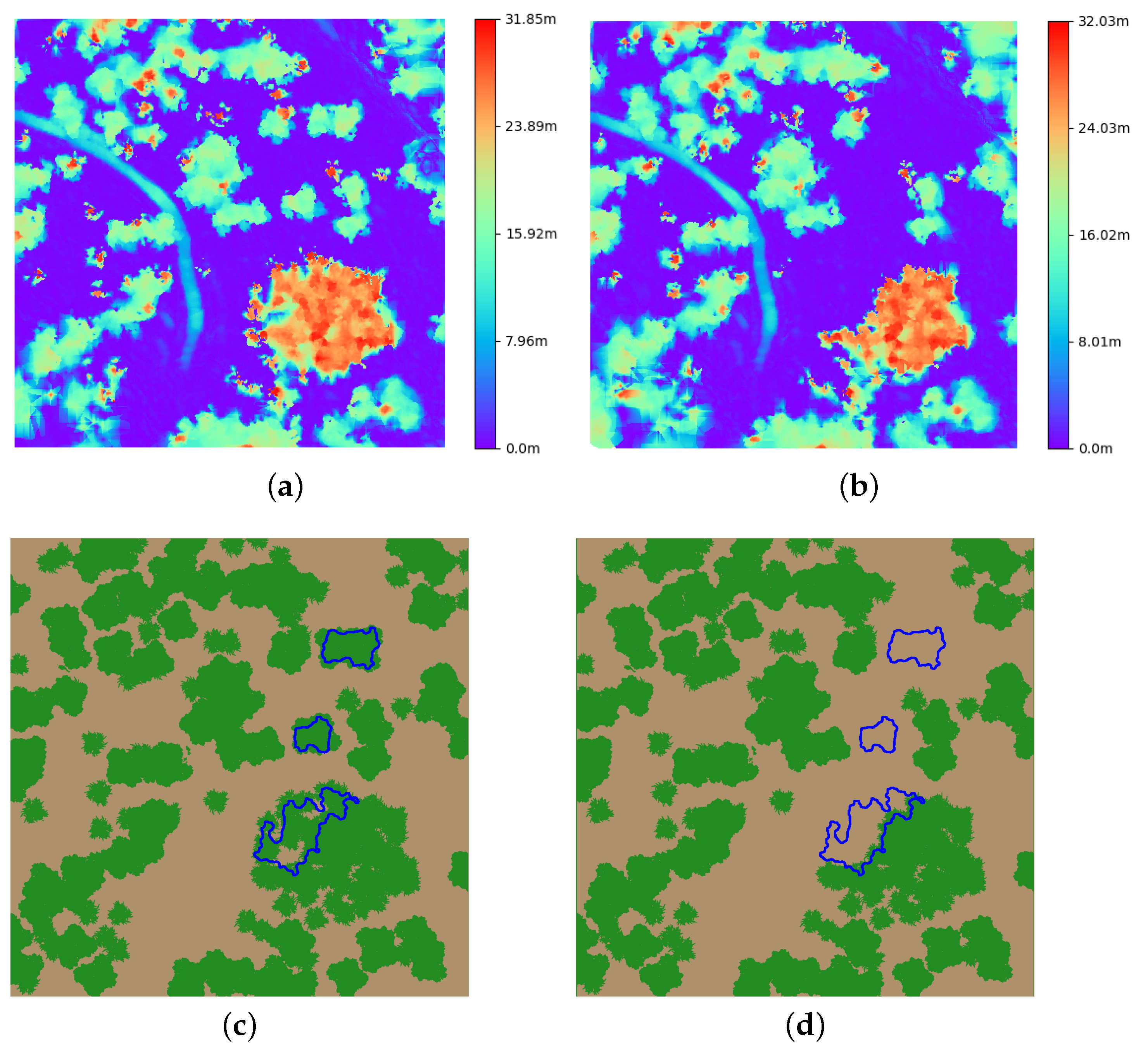
Figure 19 shows the change detection process step by step: Figure 19a,b show the resulting CHM for each mission. This covers a variety of different situations common in forests. The difference between both CHMs is computed and a binary map is generated based on a user-defined threshold. Finally, a morphological filter and contours are computed (selecting only those of a given minimum size), which gives the final result of detected changes. In this case we can observe that the three groups of removed trees are correctly detected. This can be confirmed by overlapping these contours over the scenarios with and without trees (see Figure 19c,d).
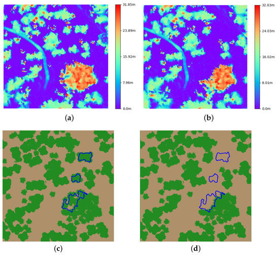
Figure 19.
Change detection process for Yosemite. (a) CHM with trees. (b) CHM without trees. (c) Scenario with trees. (d) Scenario without trees.
3.4.2. Real Word Experiments
To study the performance of our selective logging detection method in real-world conditions, a second set of experiments were performed on an area where selective logging was authorized. Due to the size of the area and safety constraints within the construction site, these experiments were carried out with the DJI Mavic 2 Pro commercial multi-rotor.
Three flights were performed at different times over two separate areas (of approximately 150 × 200 m each) in Nahuel Huapi National Park, near Villa La Angostura. Due to technical difficulties it was not possible to use GCPs for all the flights. This issue had the effect of higher drift in the absolute position of the clouds. Nevertheless, since we perform point cloud alignment this issue is easily overcome. Of course, for larger areas, GCPs would be necessary to avoid warping of the point cloud.
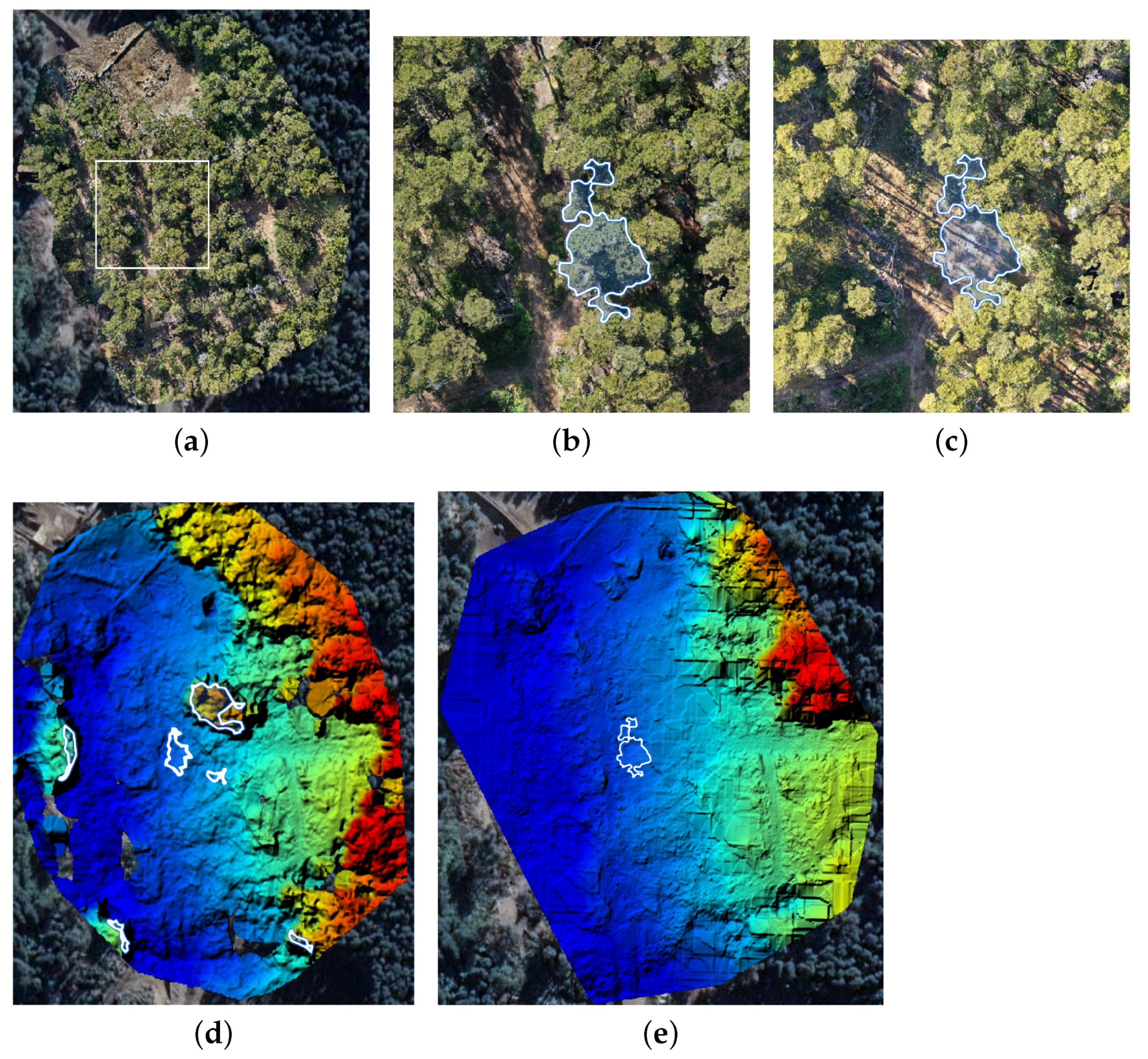
The main idea was to test the selective logging detection described in the previous section, for both cases: using the standard DTM constructed by ODM and in second place the DTM obtained using the proposed method. Figure 20a shows the original orthomosaic of the surveyed area, where some trees were cut down. Figure 20b,c show a zoom of Figure 20a (white rectangle), corresponding to the orthomosaics before and after three trees were cut down. The white lines delimit the area changed between both. To estimate this area we use the algorithm described in Section 2.7 and tested two options: (1) using the default DTM generated with ODM, or (2) using the DTM produced by the proposed method in this work.

Figure 20.
Selective logging detection algorithm applied over an area where some trees were cut down. (Top left) figure is the orthomosaic of the original area, while (middle) and (right) represent a zoom of the affected area, before and after the trees were cut down, respectively. In the (bottom) both DTM estimation are shown, whit the results of the selective logging detection algorithm highlighted in white. (a) Orthomosaic. (b) Zoom before cutting down. (c) Zoom after cutting down. (d) Original DTM. (e) Corrected DTM.
Figure 20d shows the DTM generated using the standard configuration of ODM. Comparing this image with the original orthomosaic it is possible to observe areas corresponding to trees wrongly marked as ground (yellow and red areas mostly), also the DTM presents gaps in the left and bottom parts. Using this DTM we applied the selective logging detection algorithm, and the results are shown using white lines. We observed that the method detected six areas although only the one in the center is correctly detected. On the other hand, we applied the proposed method to generate an improved DTM, the obtained result is shown in Figure 20e. The resulting DTM presents a smoother surface where most of the wrongly detected areas are now correctly classified. There is still an area on the right part showing errors, but this is because it is too close to the border of the surveyed area. We then use the selective logging detection algorithm and the results are marked in white lines. Using the corrected DTM the algorithm finds the right areas were trees were cut down.
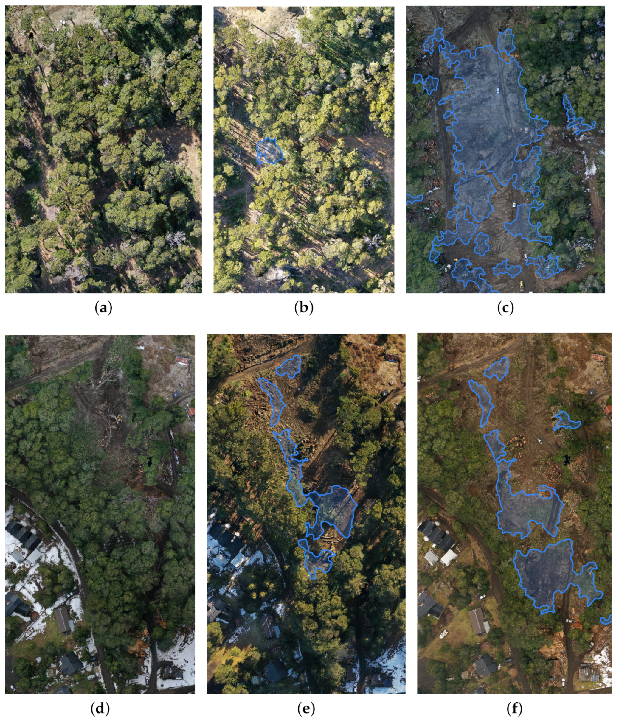
We repeated this procedure for six total survey missions in two different places, these results are shown in Figure 21. For the first area (Figure 21a–c), after the initial flight, three trees of approximately 30 m in height were cut down and, before the final flight a quite large area of trees was removed. The changes detected in the canopy structure after the second and third flight were correctly identified (marked in blue), as seen in Figure 21b,c.
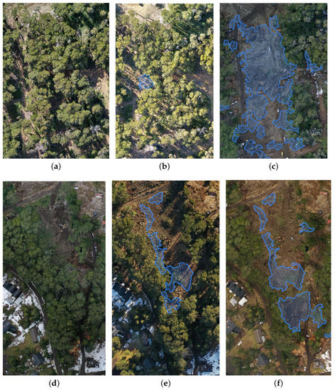
Figure 21.
Orthomosaics obtained from two flights (first flight, top row, second flight, bottom row). Leftmost image is the reference orthomosaic and the middle and the rightmost ones are from the two following flights over the same areas, after different trees were cut down. Areas detected by our detection system are highlighted in blue. (a) First survey. (b) Second survey. (c) Third survey. (d) First survey. (e) Second survey. (f) Third survey.
For the second area (Figure 21d–f), the section of trees removed is smaller and thus allows to see the performance on a more challenging case. In Figure 21e,f we show the detection results which again reflect the areas where selective logging was performed. This example also demonstrates that recognizing these changes could be quite difficult for a human, but an automated approach can be successful.
4. Conclusions
In this work we approached the problem of forest structural parameters estimation using aerial photogrammetry. We analyzed two relevant issues: the selection of survey mission and sensor settings and the generation of DTM using a camera sensor in forests. For the first issue, an exhaustive analysis is presented using a custom-built highly realistic simulator that allows experimental repeatability. For the second issue we proposed a new method to generate the DTM in forested environments using only the point cloud from SfM. Finally, we tested our method in real-world cases using different UAVs in natural forest areas.
In first place we studied the impact of flight settings in the final 3D reconstruction quality. We tested different configurations of image overlap, camera angle, flight pattern and altitude. The use of a simulator allowed us to carry out hundreds of experiments and to count with a ground-truth to compare the obtained results. For the overlap we found that it is beneficial to use the highest possible value of frontal overlap, taking into account hardware capabilities (image rate acquisition) and the required processing time. Moreover a lower value of lateral overlap is also preferred as it results in a lower number of images but with similar precision in the reconstruction. Frontal and lateral overlap of 95% and 85% respectively have shown to give the best results for forests. For the camera angle in single grid configuration a nadir angle shows better results than when using smaller angles, as the number of points is increased while RMSE is improved. In the double grid case, a combination of and angles for each flight allowed us to achieve the best results for two different overlap configurations. In relation to altitude in the simple grid case, we found that higher altitudes result in a smaller number of points and images, but also reduced precision. In the double grid case we found that the most precise reconstruction corresponds to the uses of two specific flight altitudes of m and m.
We also tested the proposed ground segmentation method for forested areas and we were able to reduce the RMSE considerably. This improvement was also reflected in the coverage percentage estimation, where the error has halved. We also performed qualitative analysis using real-world experiments with good results for both tree coverage and height.
The capability to generate the DTM in forested environments using only the point cloud from SfM is the key for UAS-based photogrammetry in cases where there is no other source available, or it is not possible to use LiDAR due to their high cost or operational difficulty. Therefore, the presented method can make UAS-based photogrammetry an available tool to a larger set of stakeholders, such as local forest management agencies, citizen science, and research projects with limited resources.
To summarize, we can conclude that UAS-based photogrammetry in forest environments is challenging but still possible and allows to obtain useful results if proper settings for mission and sensor are considered and an accurate DTM is generated. As demonstrated in this work, it can be used for structural forest parameters estimation and selective logging detection, becoming in a powerful tool for forest inventory and management. In this way, we save ourselves from tedious fieldwork, low-resolution results from satellite imagery, and expensive alternatives such as airborne LiDAR systems.
Author Contributions
Conceptualization, S.T., R.G., F.G.-F., M.N., P.D.C. and F.P.; methodology, M.N., F.P. and P.D.C.; software, F.P., F.G.-F. and N.C.; validation, F.P. and and N.C.; formal analysis, F.P. and F.G.-F.; investigation, S.T., F.P., P.D.C. and M.N.; resources, P.D.C.; data curation, F.P. and N.C.; writing—original draft preparation, S.T., P.D.C., F.P. and M.N.; writing—review and editing, S.T., P.D.C., F.P., M.N. and F.G.-F.; visualization, F.P.; supervision, P.D.C.; project administration, P.D.C. and M.N.; funding acquisition, S.T., R.G., M.N., F.G.-F. and P.D.C. All authors have read and agreed to the published version of the manuscript.
Funding
This research was funded by the Agencia Nacional de Promoción Científica y Tecnológica, Argentina and the Ministerio de Ambiente y Desarrollo Sustentable de la Nación, Argentina, under Grant number PICTO-2014-0076 and Universidad de Buenos Aires, grant code UBACYT 20020190200340BA.
Data Availability Statement
The data that support the findings of this study are available from the corresponding author upon reasonable request.
Acknowledgments
We also would like to thank the Administración de Parques Nacionales, all park rangers of the Ciervo de los Pantanos national park and specially Luis Paupy for his technical support.
Conflicts of Interest
The authors declare no conflict of interest. The funders had no role in the design of the study; in the collection, analyses, or interpretation of data; in the writing of the manuscript, or in the decision to publish the results. This publication has been approved by all the coauthors, as well as relevant authorities where data acquisition has been carried out.
References
- McRoberts, R.E.; Tomppo, E.O. Remote sensing support for national forest inventories. Remote Sens. Environ. 2007, 110, 412–419. [Google Scholar] [CrossRef]
- Torresan, C.; Berton, A.; Carotenuto, F.; Di Gennaro, S.F.; Gioli, B.; Matese, A.; Miglietta, F.; Vagnoli, C.; Zaldei, A.; Wallace, L. Forestry applications of UAVs in Europe: A review. Int. J. Remote Sens. 2017, 38, 2427–2447. [Google Scholar] [CrossRef]
- Dainelli, R.; Toscano, P.; Di Gennaro, S.F.; Matese, A. Recent advances in unmanned aerial vehicle forest remote sensing—A systematic review. Part I: A general framework. Forests 2021, 12, 327. [Google Scholar] [CrossRef]
- White, J.C.; Coops, N.C.; Wulder, M.A.; Vastaranta, M.; Hilker, T.; Tompalski, P. Remote sensing technologies for enhancing forest inventories: A review. Can. J. Remote Sens. 2016, 42, 619–641. [Google Scholar] [CrossRef] [Green Version]
- Masek, J.G.; Hayes, D.J.; Hughes, M.J.; Healey, S.P.; Turner, D.P. The role of remote sensing in process-scaling studies of managed forest ecosystems. For. Ecol. Manag. 2015, 355, 109–123. [Google Scholar] [CrossRef] [Green Version]
- Immitzer, M.; Stepper, C.; Böck, S.; Straub, C.; Atzberger, C. Use of WorldView-2 stereo imagery and National Forest Inventory data for wall-to-wall mapping of growing stock. For. Ecol. Manag. 2016, 359, 232–246. [Google Scholar] [CrossRef]
- Iglhaut, J.; Cabo, C.; Puliti, S.; Piermattei, L.; O’Connor, J.; Rosette, J. Structure from motion photogrammetry in forestry: A review. Curr. For. Rep. 2019, 5, 155–168. [Google Scholar] [CrossRef] [Green Version]
- Dash, J.P.; Watt, M.S.; Pearse, G.D.; Heaphy, M.; Dungey, H.S. Assessing very high resolution UAV imagery for monitoring forest health during a simulated disease outbreak. ISPRS J. Photogramm. Remote Sens. 2017, 131, 1–14. [Google Scholar] [CrossRef]
- Michez, A.; Piégay, H.; Lisein, J.; Claessens, H.; Lejeune, P. Classification of riparian forest species and health condition using multi-temporal and hyperspatial imagery from unmanned aerial system. Environ. Monit. Assess. 2016, 188, 146. [Google Scholar] [CrossRef] [Green Version]
- Lehmann, J.R.K.; Nieberding, F.; Prinz, T.; Knoth, C. Analysis of unmanned aerial system-based CIR images in forestry—A new perspective to monitor pest infestation levels. Forests 2015, 6, 594–612. [Google Scholar] [CrossRef] [Green Version]
- Mokroš, M.; Vỳbošt’ok, J.; Tomaštík, J.; Grznárová, A.; Valent, P.; Slavík, M.; Merganič, J. High precision individual tree diameter and perimeter estimation from Close-Range photogrammetry. Forests 2018, 9, 696. [Google Scholar] [CrossRef] [Green Version]
- Lisein, J.; Michez, A.; Claessens, H.; Lejeune, P. Discrimination of deciduous tree species from time series of unmanned aerial system imagery. PLoS ONE 2015, 10, e0141006. [Google Scholar] [CrossRef] [PubMed]
- Alonzo, M.; Andersen, H.E.; Morton, D.C.; Cook, B.D. Quantifying boreal forest structure and composition using UAV structure from motion. Forests 2018, 9, 119. [Google Scholar] [CrossRef] [Green Version]
- Dainelli, R.; Toscano, P.; Gennaro, S.F.D.; Matese, A. Recent advances in Unmanned Aerial Vehicles forest remote sensing—A systematic review. Part II: Research applications. Forests 2021, 12, 397. [Google Scholar] [CrossRef]
- Baltsavias, E.; Gruen, A.; Eisenbeiss, H.; Zhang, L.; Waser, L. High-quality image matching and automated generation of 3D tree models. Int. J. Remote Sens. 2008, 29, 1243–1259. [Google Scholar] [CrossRef]
- White, J.C.; Wulder, M.A.; Vastaranta, M.; Coops, N.C.; Pitt, D.; Woods, M. The utility of image-based point clouds for forest inventory: A comparison with airborne laser scanning. Forests 2013, 4, 518–536. [Google Scholar] [CrossRef] [Green Version]
- Leberl, F.; Irschara, A.; Pock, T.; Meixner, P.; Gruber, M.; Scholz, S.; Wiechert, A. Point clouds. Photogramm. Eng. Remote Sens. 2010, 76, 1123–1134. [Google Scholar] [CrossRef]
- Klápště, P.; Urban, R.; Moudrỳ, V. Ground Classification of UAV Image-Based Point Clouds Through Different Algorithms: Open Source vs Commercial Software. In Proceedings of the 6th International Conference on “Small Unmanned Aerial Systems for Environmental Research” (UAS4ENVIRO.2018), Split, Croatia, 27–29 June 2018. [Google Scholar]
- Pingel, T.; Clarke, K.; Mcbride, W. An Improved Simple Morphological Filter for the Terrain Classification of Airborne LIDAR Data. ISPRS J. Photogramm. Remote Sens. 2013, 77, 21–30. [Google Scholar] [CrossRef]
- Vastaranta, M.; Wulder, M.A.; White, J.C.; Pekkarinen, A.; Tuominen, S.; Ginzler, C.; Kankare, V.; Holopainen, M.; Hyyppä, J.; Hyyppä, H. Airborne laser scanning and digital stereo imagery measures of forest structure: Comparative results and implications to forest mapping and inventory update. Can. J. Remote Sens. 2013, 39, 382–395. [Google Scholar] [CrossRef]
- Wang, C.; Morgan, G.; Hodgson, M.E. sUAS for 3D Tree Surveying: Comparative Experiments on a Closed-Canopy Earthen Dam. Forests 2021, 12, 659. [Google Scholar] [CrossRef]
- Frey, J.; Kovach, K.; Stemmler, S.; Koch, B. UAV photogrammetry of forests as a vulnerable process. A sensitivity analysis for a structure from motion RGB-image pipeline. Remote Sens. 2018, 10, 912. [Google Scholar] [CrossRef] [Green Version]
- Ni, W.; Sun, G.; Pang, Y.; Zhang, Z.; Liu, J.; Yang, A.; Wang, Y.; Zhang, D. Mapping three-dimensional structures of forest canopy using UAV stereo imagery: Evaluating impacts of forward overlaps and image resolutions with LiDAR data as reference. IEEE J. Sel. Top. Appl. Earth Obs. Remote Sens. 2018, 11, 3578–3589. [Google Scholar] [CrossRef]
- Seifert, E.; Seifert, S.; Vogt, H.; Drew, D.; Van Aardt, J.; Kunneke, A.; Seifert, T. Influence of drone altitude, image overlap, and optical sensor resolution on multi-view reconstruction of forest images. Remote Sens. 2019, 11, 1252. [Google Scholar] [CrossRef] [Green Version]
- Fritz, A.; Kattenborn, T.; Koch, B. UAV-based photogrammetric point clouds—Tree stem mapping in open stands in comparison to terrestrial laser scanner point clouds. Int. Arch. Photogramm. Remote Sens. Spat. Inf. Sci 2013, 40, 141–146. [Google Scholar] [CrossRef] [Green Version]
- Díaz, G.M.; Mohr-Bell, D.; Garrett, M.; Muñoz, L.; Lencinas, J.D. Customizing unmanned aircraft systems to reduce forest inventory costs: Can oblique images substantially improve the 3D reconstruction of the canopy? Int. J. Remote Sens. 2020, 41, 3480–3510. [Google Scholar] [CrossRef]
- Nesbit, P.R.; Hugenholtz, C.H. Enhancing UAV–SFM 3d model accuracy in high-relief landscapes by incorporating oblique images. Remote Sens. 2019, 11, 239. [Google Scholar] [CrossRef] [Green Version]
- Bielova, O.; Hänsch, R.; Ley, A.; Hellwich, O. A Digital Image Processing Pipeline for Modelling of Realistic Noise in Synthetic Images. In Proceedings of the 2019 IEEE/CVF Conference on Computer Vision and Pattern Recognition Workshops (CVPRW), Long Beach, CA, USA, 16–17 June 2019. [Google Scholar]
- Koenig, N.; Howard, A. Design and Use Paradigms for Gazebo, An Open-Source Multi-Robot Simulator. In Proceedings of the IEEE/RSJ International Conference on Intelligent Robots and Systems, Sendai, Japan, 28 September–2 October 2004; pp. 2149–2154. [Google Scholar]
- Dandois, J.P. Remote Sensing of Vegetation Structure Using Computer Vision. Ph.D. Thesis, University of Maryland, Baltimore County, MD, USA, 2014. [Google Scholar]
- OpenTopography. National Center for Airborne Laser Mapping (NCALM). Forests 2013. [Google Scholar] [CrossRef]
- Leachtenauer, J.C.; Driggers, R.G. Surveillance and Reconnaissance Imaging Systems: Modeling and Performance Prediction; Artech House: Norwoord, MA, USA, 2001. [Google Scholar]
- Kazhdan, M.; Bolitho, M.; Hoppe, H. Poisson surface reconstruction. In Proceedings of the Fourth Eurographics Symposium on Geometry Processing, Cagliari, Italy, 26–28 June 2006; Volume 7. [Google Scholar]
- Cignoni, P.; Rocchini, C.; Scopigno, R. Metro: Measuring error on simplified surfaces. In Computer Graphics Forum; Wiley Online Library: Hoboken, NJ, USA, 1998; Volume 17, pp. 167–174. [Google Scholar]
- Barnhart, T.B.; Crosby, B.T. Comparing two methods of surface change detection on an evolving thermokarst using high-temporal-frequency terrestrial laser scanning, Selawik River, Alaska. Remote Sens. 2013, 5, 2813–2837. [Google Scholar] [CrossRef] [Green Version]
- DiFrancesco, P.M.; Bonneau, D.; Hutchinson, D.J. The implications of M3C2 projection diameter on 3D semi-automated rockfall extraction from sequential terrestrial laser scanning point clouds. Remote Sens. 2020, 12, 1885. [Google Scholar] [CrossRef]
- PDAL. PDAL Point Data Abstraction Library. 2018. Available online: https://zenodo.org/record/2556738 (accessed on 28 August 2020).


Publisher’s Note: MDPI stays neutral with regard to jurisdictional claims in published maps and institutional affiliations. |
© 2022 by the authors. Licensee MDPI, Basel, Switzerland. This article is an open access article distributed under the terms and conditions of the Creative Commons Attribution (CC BY) license (https://creativecommons.org/licenses/by/4.0/).