Estimation and Spatial Mapping of Residue Biomass following CTL Harvesting in Pinus radiata Plantations: An Application of Harvester Data Analytics

Abstract

The utilization of forest harvest residues for renewable bioenergy production and bioproducts has increasingly become an integrated part of forestry that helps to meet the needs of climate change mitigation and a future carbon neutral economy. An essential element in the planning of any harvesting residue recovery operation is a reliable assessment of the quantity and quality of residue biomass and its composition over a harvest area. With the now widely adopted cut-to-length (CTL) at the stump harvesting system in Pinus radiata plantations in Australia, harvesting residues left on site are significantly larger in quantity and spatially more dispersed over a harvest area in comparison to the more traditional whole-tree harvesting. The conventional approach of assessing forest harvest residues through sample plots, transects, or small study blocks has provided site-specific estimates of residue biomass. However, these estimates cannot be readily extrapolated over the plantation landscape, which varies in silviculture, site, and stand conditions. To overcome this limitation, this study relied on harvester data analytics to obtain spatially explicit estimates of residue biomass using an example data set from harvested plantations of three stand types: unthinned (T0), thinned once (T1), and thinned twice (T2). Three methods of integrating biomass equations with harvester data were compared for residue biomass estimation: (1) applying individual tree biomass equations to harvested stems, (2) applying stand-level biomass equations to gridded harvester data, and (3) integrating estimates from the first approach with recorded and estimated waste volumes of harvested stems. The estimates of total residue biomass obtained using the three methods through harvester data analytics varied between 56.2 and 156.4 t/ha in green weight across the three stand types. These estimates were validated indirectly through ex situ sample plots and proved to be comparable to the quantities of residue biomass assessed using conventional sample plots, transects, or small blocks following CTL harvesting of rotation age P. radiata plantations elsewhere in Australia. Among the three methods, the third method made the most intensive use of the harvester data and provided the most realistic estimates of residue biomass. Spatial mapping of the estimated total and component residue biomass will assist the operational planning of residue recovery and site-specific nutrient management for the long-term sustainability of P. radiata plantations.

1. Introduction

The utilization of forest harvest residues in managed forests for the production of renewable bioenergy and bioproducts has increasingly become an integrated part of forestry that helps to meet the needs of climate change mitigation and a future carbon neutral economy [1,2,3,4,5,6,7,8,9,10]. An essential element in the planning of any residue recovery operation, either stand alone or integrated with conventional log harvesting, is a reliable estimation and assessment of the quantity and quality of residue biomass and its composition over a harvest area [11,12,13]. After a plantation is harvested at rotation age for high-value timber and wood-fibre products, there is usually a large amount of low-value residue material lying scattered on the forest floor. The harvest residues mainly consist of stumps, branches, and treetops, as well as short offcut and waste sections due to stem deformity, defects, damage, and breakage. They may also include standing broken stems and standing dead trees if left unharvested. With the now widely adopted cut-to-length (CTL) at the stump harvesting system, residues left on site are significantly larger in quantity and spatially more dispersed over a harvest area in comparison to the more traditional whole-tree harvesting, whereby trees are delimbed and bucked at the landing site [12,14,15]. In addition to providing environmental benefits, residue recovery following CTL harvesting would reduce the intensity of post-harvest residue management and thereby minimize the cost of site preparation for the next rotation, particularly where residue levels are high [11,16,17].

With a total planted area well exceeding 4.2 million hectares worldwide, and still expanding, Pinus radiata (D. Don) is the most extensively planted exotic coniferous species in four Southern Hemisphere countries (Australia, Chile, New Zealand, and South Africa) and in one country north of the equator (Spain) [18,19]. In these countries, P. radiata plantations are the mainstay of the forest economy, producing logs for export and a wide range of timber and wood-fibre products for the domestic markets. In any region of industrial scale production, the year-round harvesting of rotation-age plantations provides a continuous flow of sawlogs and pulpwood, and, at the same time, a continuous potential supply of residue biomass for bioenergy generation. In Australia, the current P. radiata plantation estate is approximately 780,000 ha and about one-third of this resource is in the State of New South Wales (NSW) [20]. Several studies in P. radiata plantations have shown that the green weight of harvest residues on CTL clearfell sites ranged from less than 50 t/ha to more than 300 t/ha [12,21,22,23]. In the past, post-harvest residues were usually windrowed, burned, and mostly reduced to ashes to return to the soil as part of site preparation for the establishment of the next rotation. Nowadays, the residues are increasingly recovered and utilized as a feedstock for bioenergy production, avoiding windrowing and burning on site and thereby minimizing the cost of re-establishment [8,13,24,25].

The total amount of residue biomass on the forest floor following harvesting and its composition in terms of stumps, branches, tree-tops, and short offcut and waste sections vary spatially at multiple scales across stands with different site and stand conditions, different silvicultural regimes, and natural disturbance histories [11,22,23]. For unthinned P. radiata stands harvested at rotation age, a greater proportion of total residue biomass was found to be in the waste component and a smaller proportion in the branches in comparison to thinned stands [23]. Unlike commercial logs, the spatially more dispersed harvest residues are low in biomass density and economic value but high in volume, collection, and transportation cost [13]. Out of the total amount of residues that are potentially available for collection in a harvest area, the proportion of recoverable residues depends on their collection costs, which are a function of the distance from roadside landing, terrain conditions, collection method, their moisture content, and degree of drying [13,26,27]. Among these factors, the spatial location or distribution of residue biomass provides the basis for such distance-dependent cost calculations.

Up until now, estimation of residue biomass has relied on either plot or transect-based sampling or on assessment of small study blocks between 0.5 and 5.0 ha in size (e.g., [15,22,28]). Another approach has been to predict residue biomass at either the individual tree or stand level from tree or stand variables derived from pre-operational inventory plots. For rotation age P. radiata plantations grown under different thinning regimes, systems of equations have been developed specifically to estimate the biomass in commercial logs and harvest residues in fresh and dry weight at both individual tree and stand levels [23,29]. The inventory and sampling-based estimates are then scaled up on a pro rata basis to provide estimates of total and recoverable residue biomass for a harvest area or a plantation estate. Such scaled-up estimates, although useful for broad, high-level management planning, lack the spatial resolution for more detailed operational planning that considers the collection and transportation costs. At an operational level, reliable and spatially explicit estimation of residue biomass and its composition is needed to assist planning for clearfell operations that integrate conventional CTL harvesting with residue biomass collection—i.e., integrated biomass recovery (e.g., [30,31]).

Since CTL harvesters were introduced into Australia for plantation harvesting in the early 1990s [32], cut-to-length at the stump has become the predominant harvesting system used in the country [13]. The present-day CTL harvesters are equipped with an on-board computer and a GPS receiver together with a computerized harvester head to optimize cutting and thereby reduce volume of waste and simultaneously collect production data in real time during harvesting. A harvester dataset usually contains anywhere between tens of thousands and millions of stems. The assortment, length, and end diameters of each log and waste section cut from each stem were recorded together with its spatial location, time stamp, and many other variables associated with harvesting operation and log production (see [33,34]). However, stump height and total tree height are not available because the harvester head does not process the stump and the treetop beyond the last cutting point and so cannot measure their lengths. Nonetheless, the spatially explicit and comprehensive log production data, when combined with biomass equations developed specifically for rotation age stands (e.g., [23,29]), would help overcome the limitations of conventional plot or transect-based sampling in the estimation of residue biomass. This approach of using harvester data to estimate residue biomass was adopted for the most common Scandinavian tree species in Finland [35,36,37]. Most recently, Woo et al. [38] developed a software tool attempting to integrate harvester data and individual tree biomass equations for the estimation of residue biomass, but the estimates they demonstrated for a patch of P. radiata plantation in Tasmania, an island state of Australia, were out of the range in comparison with previously reported residue and total aboveground stand biomass for P. radiata plantations in Australia [21,22,23,39,40,41].

For more reliable estimations of log product and residue biomass, the DBHOB (diameter at breast height overbark) and total tree height of the bucked stems contained in a harvester dataset need to be estimated first using predictive equations developed specifically for this purpose (see [42,43]). Further, the spatial locations of stems and their estimated DBHOB and height can be used to calculate the stand level attributes such as stand density, basal area, and stand height of tessellated grid cells or otherwise defined areas (e.g., [44,45,46,47]). As predictors for biomass, these tree and stand attributes provide an essential linkage between harvester data and biomass equations at both the tree and stand levels. A case in point is the systems of equations developed by Wang et al. [29] and Qiao et al. [23] for predicting biomass in commercial logs and residue components for the rotation age P. radiata trees and stands. When such biomass equations are applied to harvester data from P. radiata plantations, their applicability and limitations for predicting component biomass need to be evaluated and recognised. The need to do so arises from the fact that biomass equations are usually based on a limited number of sample trees with stems largely free from defects and, consequently, their cutting patterns during destructive sampling tend to be more regular than those encompassed in a big harvester dataset. At least for some stems in harvester data, the proportional biomass allocated to commercial logs and waste sections, a major component of residue biomass, may differ substantially from the allocation patterns covered by the limited number of sample trees for developing biomass equations.

This study aimed to introduce harvester data analytics for the estimation and spatial mapping of residue biomass in plantations following CTL harvesting and to demonstrate the usefulness of this novel approach in overcoming the limitations of the conventional inventory and sampling-based residue biomass estimation. In doing so, recently harvested P. radiata plantations that underwent three different thinning regimes were used as examples. Three approaches were adopted and compared for accomplishing the objective: (1) applying individual tree biomass equations to stems contained in the harvester data, (2) linking stand level biomass equations to gridded harvester data, and (3) refining estimates of component biomass for individual trees using the cutting pattern, log, and waste volumes of each bucked stem in the harvester data. As standing dead trees in a plantation are not logged in harvester data during harvesting, adjustment factors were determined and incorporated for thinned and unthinned stands when the refined individual tree estimates were aggregated and scaled up to the stand level. The residue biomass that was calculated through the three methods were validated indirectly and compared with previously reported conventional estimates of residue biomass in P. radiata plantations elsewhere. The comparative results led to recommendations on the best approach for the estimation and spatial mapping of residue biomass to assist harvest planning for operations that integrate CTL log production with residue biomass collection in P. radiata plantations.

2. Study Area

The study area was within the Bathurst management area of the Forestry Corporation of New South Wales (FCNSW), the largest manager of P. radiata plantations in Australia. This management area encompasses a total of 70,000 hectares of P. radiata plantations across 18 disjunct state forests, spreading across an east–west distance of about 130 km and a north–south distance of about 190 km on the central west slopes of NSW. Its geographical location, geology, soil types, climatic and site conditions, history of plantation establishment, and the silvicultural regimes and rotation ages of the plantations were described in detail by Knott and Ryan [48], Wang et al. [29], and Qiao et al. [23]. Since the 1980s, the initial planting stocking has been set to 1000–1300 trees/ha, except for steeper slopes where stands are established with a lower stocking of 700–900 trees/ha and no thinning operation is intended [49]. For more productive sites, either one or two thinnings are prescribed to reduce the stocking down to 450–550 trees/ha at the age of first thinning, which is around 14 years, and down to 200–300 trees/ha at the age of second thinning, which is around the age of 23 years. However, the prescribed thinning regime may be applied to a plantation with some necessary variations because the decision to thin a particular area is also dependent on other factors, such as drought exposure, tree health, customer product requirements, and economic and market considerations [49]. For poorer sites, no thinning is specified before the final harvest, which is generally at the rotation age of 30 to 35 years.

3. Harvester Data

As part of a larger harvester data analytics project, harvester data from recently harvested P. radiata plantations across nine state forests in the Bathurst management area were screened, cleaned, and processed through a workflow based on previously established protocols and procedures [42,43]. The harvesters currently operating in the Bathurst management area are mostly tracked John Deere, Komatsu, Tigercat, and Timberpro base machines with a 9–10 m boom reach. They are fitted with a Waratah or Komatsu harvesting and processing head together with Waratah’s TimberRite^TM or Komatsu’s MaxiXplorer^TM control, measurement, and information system. These harvesters are still using the old ASCII-based StanForD (Standard for Forest Machine Data and Communication), which was originally developed by the Forestry Research Institute of Sweden in 1988 [50], and not the new xml-based StanForD2010 released in 2011 [33,51]. Machine operators are required to calibrate their harvester heads on a regular basis through standard procedures according to the guidelines of FCNSW. An unpublished internal study on the accuracy of calibrated harvester heads showed the mean error of log length measurements for a 5 m log was 0.11 cm and the percentage of logs within the 6 adjacent 1 cm error classes with the highest number of logs was 90.1%. For a log end with a DOB of 30 cm, the mean measurement error of DOB ranged from −0.3 to 0.05 cm depending on the log positions. Following harvesting, all information recorded and stored in the onboard computer of each harvester was uploaded to the harvester database management system of FCNSW through the STICKS software developed by ForestPHD Pty. Ltd., Rotorua, New Zealand, which is widely used in Australia at present.

The harvester data contained the length, small end diameter overbark (SEDOB), and volume overbark of every log and waste section cut from each stem. In addition, log assortment was recorded according to customer product specifications. Offcut sections were tagged as waste in product assortment regardless of their lengths. SEDOB was recorded in mm, log length in cm, and overbark log and waste volume in m³, but DBHOB was not contained in the harvester data. The latitude and longitude of each stem were in the harvester data. Given that the GPS receiver is mounted on the cabin of harvesters, the recorded spatial location was the position of the harvester cutting the tree but not that of the tree itself. The actual position of the tree relative to the harvester could be anywhere within the range of the boom in any direction as the boom orientation could not be measured. Such positional error for a tree was compounded with the GPS receiver error for the harvester. When the accuracy of the GPS receivers in a forest environment was taken into account, the positional error for the individual stems was expected to be in the typical range of 10–20 m, as assessed by Lindroos et al. [52]. For the objectives of this study, a small subset of data was selected and extracted from the larger harvester dataset to represent plantations of three stand types: unthinned (T0), thinned once (T1), and thinned twice (T2). These plantations were all established in 1988 and harvested over a period of ten months between April 2020 and February 2021. The plantations consisted of 19 disjunct patches with a total area of approximately 136 ha and 74,094 harvested stems. There were 9 patches of T0 plantations varying between 2.4 and 9.4 ha with a total area of 46.4 ha, 5 patches of T1 plantations varying between 2.5 and 31.5 ha with a total area of 48.0 ha, and 5 patches of T2 plantations varying between 5.8 and 11.4 ha with a total area of 41.4 ha. The disjunct patches of each stand type were within close proximity to each other as they belonged to the same State Forest in the study area.

4. Harvester Data Analytics

The entire process of harvester data analytics started from data exploration, diagnostics, tagging, and screening. This initial data processing was carried out in multiple rounds and was facilitated through descriptive as well as diagnostic data analysis and visualization. In each round, the exploratory analysis and data screening detected data errors, discovered duplicated records, and uncovered problems with variables in different ways. After this, necessary steps were taken to correct data errors and rectify problems. As this initial phase of data processing was carried out as part of the larger harvester data analytics project across the nine state forests in the Bathurst management area, detailed descriptions would be lengthy and beyond the scope of this paper. After the harvester data were cleaned and tidied up, the following major steps were carried out: (1) reconstructing the size of individual trees, (2) calculating stand-level attributes using gridded harvester data, (3) estimating residue biomass by applying biomass equations at both individual tree and stand levels and also through converting the recorded log and waste volumes of stems into biomass, and (4) producing residual biomass heat maps for the harvested areas.

4.1. Reconstructing the Size of Individual Trees

Following the screening and pre-processing of the harvester data, the DBHOB and total tree height of each bucked stem were estimated using equations previously developed by Lu et al. [42] and Shan et al. [43] for the purpose of processing harvester data from P. radiata plantations. DBHOB was estimated from the SEDOB and the height above ground-level of the butt log, which was calculated as the length of the butt log plus a stump height of 0.15 m. This stump height was the average height of more than 4600 stumps measured in post-harvesting surveys over 31 sites as part of the routine residue assessment for clearfell operations using CTL harvesters in P. radiata plantations in NSW [42]. A set of simple linear regression equations and correction factors for log transformation bias was tabulated by Lu et al. [42] for estimating DBHOB at specified heights between 0.05 and 7.05 m above ground-level with an interval of 0.1 m and between 7.05 and 9.55 m with an interval of 0.5 m. The total tree height of bucked stems was estimated using the nonlinear equations developed by Shan et al. [43]:

$$\mathrm{H}=\frac{{\mathrm{L}+\mathrm{H}}_{\mathrm{s}} - 1.3}{{\left(1 - \mathrm{d}\right)}^{{\mathrm{a}}_1{+\mathrm{a}}_2{\mathrm{L}+\mathrm{a}}_3\sqrt{\mathrm{T}}{+\mathrm{a}}_4\sqrt{{\mathrm{d}}^3}{+\mathrm{a}}_5\sqrt{{\mathrm{DBHOB}}^3}}}+1.3$$

(1)

and

$${\mathrm{H}=\mathrm{H}}_{\mathrm{S} }{+\mathrm{L}+\mathrm{L}}^{{\mathrm{b}}_3}{\mathrm{DBHOB}}^{{\mathrm{b}}_4}{\mathrm{SEDTL}}^{{\mathrm{b}}_6}{\mathrm{e}}^{{\mathrm{b}}_1{+\mathrm{b}}_2{\mathrm{L}+\mathrm{b}}_5\mathrm{SEDTL}}$$

(2)

where H is the total tree height from ground level to tip in m of a stem, L is its total log length in m—i.e., the sum of lengths of all logs and waste sections cut from the stem—H_s represents the stump height of 0.15 m, SEDTL stands for the SEDOB of the top log in cm, $\mathrm{d}=(\mathrm{SEDTL}⁄\mathrm{DBHOB})$ is the relative diameter in the unit interval of (0, 1), $\mathrm{T}=\left(\mathrm{DBHOB}-\mathrm{SEDTL}\right)/\mathrm{L}$ is the average taper of the cut stem in cm/m, and a_i and b_i are parameters. For stems with d ≤ 0.8, Equation (1) was used because its predictive performance was superior to that of Equation (2) within this relative diameter range. When d > 0.8, Equation (2) was used as its performance was slightly better than that of Equation (1) [43].

4.2. Delineation and Tessellation of Harvester Data for Calculating Stand Level Attributes

The spatial boundaries of each harvest area were delineated by computing in QGIS an alpha convex hull of all stem positions using the method of Asaeedi et al. [53], which uses polygons and angles to find the shape of the hull. The convex polygon was the minimum area that included all stems in the area, but it did not account for the crown extension and the positional error of stems on the polygon borders or forest edges. More than 99% of the harvested stems across the three stand types had an estimated DBHOB less than 65 cm. For open grown P. radiata of the same diameter, the maximum crown extension would be about 7 m, as calculated from the linear relationship between crown width and DBHOB derived by Leech [54]. The boom reach of harvesters operating in the management area ranged from 6.5 to 10.3 m, but was mostly in the range of 9–10 m. To account for the maximum crown extension of edge trees and the positional errors of their stems, a 7 m buffer was added to the polygon borders (Figure 1).

The areas covered with harvester data were tessellated initially into regular grid cells of 25 m × 25 m, 50 m × 50 m, and 100 m × 100 m in size. The three grid sizes were compared in a preliminary analysis of the harvester data. Based on the comparisons, the grid cell size of 50 m × 50 m was chosen for all three stand types (T0, T1, and T2) due to consideration of (1) the positional error of tree locations in the harvester data and (2) the number of trees in a grid cell that was adequate for calculating the stand level attributes. At rotation age, the density of thinned P. radiata stands in the management area could be less than 200 trees/ha in certain places [29]. In such cases, grid cells smaller than the chosen size would not contain enough number of trees for the calculation of stand density, basal area, and stand height. For other types of forests reported in the harvester data literature, segmentations and grid cells smaller or larger than 0.25 ha have been used (e.g., [44,46,55,56]).

All trees within a grid cell were allocated to that cell for the calculation of stand-level attributes including stand density, basal area, and stand height, which is customarily defined as the mean height of the 100 largest diameter trees/ha, calculated on a pro rata basis. These three stand variables together with stand age and stand type are the predictor variables in the systems of biomass equations that were recently developed for rotation-age P. radiata stands in the management area [23]. For grid cells that were completely within the delineated harvest area, a uniform area of 0.25 ha was used in the calculations. For partial grid cells along the boundaries of a delineated harvest area (Figure 1), the stand variables were calculated in two ways, depending on the number of harvested stems within the grid cell. For grid cells with at least 35 stems, the calculations were based on the partial area of each grid cell that was within the delineated harvest area. This number of trees was greater than the number of trees contained in a routine pre-operational inventory plot in the plantations. It was also above the minimum number of trees that was required for the reliable estimation of stand attributes (c.f. [57,58,59]). For grid cells with less than 35 trees, the width of the grid cell was stretched both vertically and horizontally by 5 m on each side to take in a greater number of stems. If still not enough, this step was repeated one or two times until there was enough of a number of trees contained in the stretched grid cell (Figure 1). The stand-level variables were then calculated using the partial area of the stretched grid cell that was within the harvest area.

4.3. Residue Biomass Estimation

Three approaches were compared for estimating residue biomass in both green and dry weight: (1) applying individual tree biomass equations to the estimated DBHOB and total tree height values of harvested stems, (2) applying stand-level biomass equations to the gridded harvester data, and (3) integrating estimates from the first approach with waste volumes of stems in the harvester data. In the first approach, the biomass of commercial logs and harvest residues were predicted for individual stems using the systems of additive and allocative equations developed by Wang et al. [29] for individual trees of P. radiata at rotation age. These equations were based on data from 239 trees that were destructively sampled from among 61 sample plots established across the three stand types in the same study area. The predictor variables in the equations were DBHOB, total tree height, and two dummy variables for the three stand types (T0, T1, and T2). For each stem, the total residue biomass was estimated first through the three additive equations for log product, harvest residue, and total aboveground biomass. Then the estimated total residue biomass was allocated to the stump, branch, and waste components through the three allocative equations (see [29]). In the second approach, the systems of six additive equations developed by Qiao et al. [23] for predicting stand-level biomass in sawlogs, pulpwood, stumps, branches, waste sections, and total aboveground biomass were applied to each grid cell over the gridded harvester data as demonstrated in Figure 1. These additive equations were developed using stand-level biomass estimates obtained for the same 61 sample plots as described above. These stand-level biomass estimates included both live trees and the standing dead trees that were found primarily in unthinned stands. For standing dead trees, either whole or broken, the stem biomass was allocated to the stump and waste components, while branch biomass was regarded as negligible and not included in the biomass calculations as described in Qiao et al. [23]. The predictors of the six additive equations included stand age, stand density, basal area, stand height, and the dummy variables for stand types.

In the third approach, the total overbark volume of commercial logs and that of the waste sections cut from a stem were calculated using the product assortment and volume information contained in the harvester data. The calculated volumes were converted to biomass in green as well as dry weight for the stem by using volume-to-biomass conversion factors. Two conversion factors were derived from the units of kg/m³ for each stand type for green and dry weight conversions, respectively. They were 789 and 413 for unthinned stands, 892 and 398 for T1 stands, and 876 and 408 for T2 stands. These conversion factors were the average biomass-to-volume ratios calculated using the fresh and dry weight and overbark volume of the whole merchantable stem (i.e., not including the stump and the top stem section beyond the last cutting point) of a total of 239 trees sampled across the three stand types in rotation age P. radiata plantations in the study area. The green and dry weight of the different biomass components of individual sample trees were calculated by Wang et al. [29] and described in detail therein. The overbark merchantable stem volume of each sample tree was derived using the overbark stem taper equation developed by Wang et al. [29] for each stand type using the trigonometric variable-form taper model form of Bi [60].

However, the waste sections and volumes recorded for a stem in the harvester data might not be all there was for the stem. This was because the harvester operators tended not to process a stem any further after cutting the last commercial log from the stem, leaving one or more potential waste sections in the upper stem unaccounted for in the harvester data. The SEDTL (SEDOB of the top log) distribution of stems in the harvester data had a lower quartile of 11.4 cm, a median of 13.3 cm, a mean of 15.8 cm, an upper quartile of 17.1 cm, and a 90th percentile of 23.2 cm, which were all greater than the minimum SEDOB of 8 cm that was specified for a pulp log. Such a positively skewed distribution indicated that a substantial proportion of trees had unprocessed stem tops that could be included as waste sections in the residue biomass calculation. To do so, the SEDTL of each bucked stem was evaluated against the minimum SEDOB for a pulp log. If it was greater than 8 cm, the overbark volume of the top stem section between the height of the last cut and the height of the minimum SEDOB was calculated through numerical integration of the overbark stem taper equation developed by Wang et al. [29] for each stand type. The volume was then converted to fresh as well as dry weight using the corresponding conversion factors as described above and included as the additional waste biomass for the stem.

As the second approach provided stand-level residue biomass estimates for individual grid cells, the three approaches for residue biomass estimation were compared at the scale of the grid cells. For the first and third methods, the residue biomass estimates of individual trees within the same grid cell were summed up and converted to stand-level estimates on a per hectare basis. Unlike the second approach, residue biomass estimates obtained through the first and third methods did not include standing dead trees, as they were not harvested and processed through the harvester head and so were not present in the harvester data. As a further refinement of the third method, its stand-level estimates of stump and waste biomass in both green and dry weight for unthinned stands in T0 grid cells were expanded by a factor of 1.10 and 1.13, respectively. These two factors were derived using stand-level biomass data calculated and compiled by Qiao [23], which contained the stump and waste biomass of both live and dead trees for the 61 sample plots across the three stand types. For each plot, a ratio of the total waste biomass of live and dead trees to that of live trees only was calculated in fresh weight. In the same way, a ratio for stump biomass was calculated. The average ratio for each residue component among the ten unthinned plots of comparable stand age to the plantations in this study was taken as the expansion factor for the T0 stands. As there were very few standing dead trees among the sample plots in the T1 and T2 stands, the calculated biomass expansion factors took the value of one after being rounded to two decimal places. Therefore, no adjustment was made to the residue biomass estimates for T1 and T2 grid cells. After the stand-level estimates were finalized, statistical graphics and simple descriptive statistics were used to compare the differences in the scaled-up estimates among the three approaches across the three stand types.

4.4. Spatial Mapping of Residue Biomass Estimates

Using the geographic locations of the harvested stems, the estimated total and component residue biomass were spatially mapped in the form of heatmaps for visualization of each harvest area. The heatmap renderer and its underlying processing algorithm in QGIS were used for this purpose. In addition, grid cell maps were made to show the quantity of total residue biomass and its proportional allocation to the stump, branch, and waste components for delineated harvest areas across the three stand types.

5. Evaluation of the Accuracy of Residue Biomass Estimation

As the harvester data analytics described above were performed for several months to a year after the routine harvesting operations, in situ data of residue biomass were not available for directly validating the calculated and spatially mapped residue biomass in the harvested plantations. In an ideal world, at least 30 survey plots of the same size as the 50 m × 50 m grid cells would need to be established and measured to obtain the tree and stand attributes for each of the three stand types prior to harvesting. During the operations, all harvest residues within a plot would have to be collected, sorted out into piles of different components, and weighed instantaneously after trees were felled and processed to avoid any substantial loss of moisture in the determination of their fresh weights. In addition, samples would have to be collected to determine the dry-to-fresh weight ratio of each component. This conventional approach of direct validation would require a large amount of time, manpower, and additional machinery working on site in synchronization with the harvester and forwarder in routine harvesting operations at a landscape scale. Such a requirement can prove to be restrictive or even prohibitive in terms of cost and operational complexity in practical situations, especially when research funding is limited. Consequently, this conventional approach has seldom been adopted. The only such example has been the case study reported by Palander et al. [36] and Vesa and Palander [37] in central Finland, where they used harvester data to estimate the stump biomass with attached roots of small to medium Norway spruce trees, mostly with DBH less than 40 cm in mixed-species stands.

To overcome the lack of in-situ data for direct validation, an alternative indirect approach was formulated to evaluate the accuracy of residue biomass estimation through using the 61 ex-situ sample plots established in rotation-age P. radiata stands in the same study area as described previously in the section on residue biomass estimation. Among the 61 plots, there were 31 plots in unthinned (T0) plantations and 15 plots each in T1 and T2 plantations. These plots were circular and generally had a radius of 15, 20, or 25 m for T0, T1, and T2 stands. The radius was varied in order to take in at least 30 to 40 trees in all the plots across the three stand types. For these plots, four stand attributes were tabulated and displayed graphically in Wang et al. [29] and Qiao et al. [23], including stand density, basal area, height, and age. The biomass in commercial logs and residues in both fresh and dry weight were calculated and scaled up to per hectare values by Qiao et al. [23] for developing the stand-level biomass equations. This data set would naturally serve as an alternative basis for the indirect validation of the residue biomass estimates obtained for the grid cells through harvester data analytics.

However, the quantities of biomass of the sample plots were not directly comparable to the estimated biomass of the grid cells. The sample plots and grid cells had different spatial scales as well as different stand attributes. To overcome these differences, two further steps of harvester data analytics were taken. Firstly, virtual plots of the same shape and size to the sample plots were drawn over the T0, T1, and T2 harvest areas using the spatial locations of individual stems as plot centres through a computer program. Not all virtual plots drawn in such a way fell completely within the boundaries of the harvested areas. Once partial plots at the edges were excluded, the number of virtual plots was greater than 21,000 for T2 stands and greater than 31,000 for T0 and T1 stands, respectively. For every virtual plot, stand attributes and biomass quantities were calculated and scaled up to per hectare values in correspondence with the data content and structure of the 61 sample plots as described above. In the second step, for each sample plot of a particular stand type, a virtual plot was selected from among all the virtual plots of the same stand type to match its stand attributes as closely as possible. To facilitate the selection process, a normalized similarity index (SI) was calculated for every virtual plot as follows:

$$\mathrm{SI}=\sqrt{{\left(\frac{\log \left({\mathrm{N}}_{\mathrm{s}}\right)-\log \left({\mathrm{N}}_{\mathrm{v}}\right)}{\log \left({\mathrm{N}}_{\max }\right)} \right)}^2+{\left(\frac{\log \left({\mathrm{G}}_{\mathrm{s}}\right)-\log \left({\mathrm{G}}_{\mathrm{v}}\right)}{\log \left({\mathrm{G}}_{\max }\right)} \right)}^2+{\left(\frac{\log \left({\mathrm{H}}_{\mathrm{s}}\right)-\log \left({\mathrm{H}}_{\mathrm{v}}\right)}{\log \left({\mathrm{H}}_{\max }\right)} \right)}^2}$$

(3)

where log stands for common logarithm; ${\mathrm{N}}_{\mathrm{s}}$, ${\mathrm{G}}_{\mathrm{s}}$, and ${\mathrm{H}}_{\mathrm{s}}$ represent the stand density, basal area, and stand height of the sample plot; ${\mathrm{N}}_{\mathrm{V}}$, ${\mathrm{G}}_{\mathrm{V}}$, and ${\mathrm{H}}_{\mathrm{V}}$ are the corresponding stand variables of a virtual plot; and ${\mathrm{N}}_{\max }$, ${\mathrm{G}}_{\max }$, and ${\mathrm{H}}_{\max }$ stands for the maximum values of the respective stand variables of all the virtual plots belonging to the stand type. Stand age was not incorporated in the formulation of SI in Equation (3), although it was one of the predictor variables in the stand-level biomass equations of Qiao et al. [23]. In comparison to the other three stand variables, differences in stand age between the sample and virtual plots only varied within a discrete and much narrower range of several years. The small differences in stand age generally resulted in a less than 1% difference in the predicted values of all the biomass components when holding constant the values of the other three stand variables in the biomass equations of Qiao et al. [23]. Including stand age in the formulation of SI would only add to the complexity of its calculation but make little difference in the calculated values. The normalization was intended to scale the values of SI between 0 and 1 within a unit cube where no single stand variable could exert a disproportional influence. For each sample plot, the virtual plot with the smallest SI, and so the closest similarity, was selected as its matching plot for the intended indirect validation (Figure 2).

Although being the closest match, the sample plot and its virtual counterpart still differed somewhat in their stand attributes (Figure 3). The differences in stand attributes would naturally translate into differences in the quantities of all biomass components between the sample and virtual plot, which would consequently confound the validation results. To minimize the confounding effects, an adjustment factor was incorporated in calculating the difference in biomass between the sample and the virtual plot during validation:

$$\epsilon =M_S-\theta M_V$$

(4)

where $M_S$ and $M_V$ represents the quantities of a certain biomass component at stand level in t/ha for the sample and the virtual plot, respectively, $\epsilon$ is the adjusted difference between $M_S$ and $M_V$, and $\theta$ is the adjustment factor, which was derived as follows:

$$\theta =\frac{f\left(N_S, G_S, H_S, A_S \right)}{f\left(N_V, G_V, H_V, A_V \right)}$$

(5)

where $f(·)$ represents the stand level equation for the biomass component as given in Equation (7) of Qiao et al. [23], $A_S$ and $A_V$ are the stand age in years of the sample and the virtual plot, respectively, and the other predictors of $f(·)$ were previously defined in Equation (3). If the sample and the virtual plot had the same predictor values, $\theta$ would be 1 and no adjustment would be made. In other cases, $\theta$ would be either slightly greater or smaller than 1 depending on how the predicted value of the biomass for the sample plot in the numerator weighed against that for the virtual plot in the denominator.

The adjusted difference $\epsilon$ was taken as the ‘error of estimation’ of the biomass component in the indirect validation of the biomass estimates obtained through harvester data analytics for the virtual plot. The size, direction, and dispersion of the estimation errors were summarized through four benchmarking statistics, including the mean error of estimation (MEE), the mean percentage error of estimation (MPEE), the mean absolute error of estimation (MAEE), and the mean squared error of estimation (MSEE). Another simple statistic, the coefficient of estimation efficiency ($R_E^2$) from [61] was also calculated to provide a simple measure of estimation performance. These statistics were calculated as follows:

$$MEE={\sum }_i^n{\epsilon }_i/n$$

(6)

$$MPEE=100\left({\sum }_i^n\left({\epsilon }_i/M_{Si}\right)\right)/n$$

(7)

$$MAEE={\sum }_i^n\left|{\epsilon }_i\right|/n$$

(8)

$$MSEE={\sum }_i^n{\epsilon }_i^2/n$$

(9)

$$R_E^2=1-\left({\sum }_i^n{\epsilon }_i^2/{\sum }_i^n{\left(M_S-{\overline{M}}_S\right)}^2\right)$$

(10)

where ${\epsilon }_i$ is the ‘error of estimation’ of the biomass component for the $i$th plot in t/ha, $n$ is the number of sample plots, and ${\overline{M}}_S$ is the average quantity of the biomass component for all $n$ sample plots. These statistics have been commonly used in evaluating the predictive performance of forest and other empirical models. In particular, the MSEE is a common measure of estimation accuracy in the statistical literature since it incorporates both the bias and variance of estimation [62]. The Nash–Sutcliffe coefficient of estimation efficiency ($R_E^2$) is sometimes referred to as ‘modelling efficiency’ or the ‘prediction coefficient of determination’ (e.g., [63,64,65,66]). It is analogous to the coefficient of determination R², which ranges from 0 to 1. However, $R_E^2$ can range from −∞ to 1 [61]. When $R_E^2<$0, the estimated values shift further away than the observed values from the observed mean and so the variance of the estimation error is larger than the variance of the observed data. Four sets of benchmarking statistics were calculated: a general set for all stand types combined by taking the number of sample plots $n$ = 61 and one set for each of the three stand types. In addition to the benchmarking statistics, the values of $M_S$ were plotted against that of $M_V$ with a line of unity slope passing through the origin for a graphical evaluation of the accuracy of residue biomass estimation.

6. Results

6.1. Tree and Stand Attributes Obtained through Harvester Data Analytics

For the 74,094 stems in the harvester data, the estimated DBHOB ranged from 8.3 to 74.7 cm and the estimated total tree height varied from 7.7 to 46.6 m. The range of tree size was similar across the three stand types because of the large number of trees in the harvester data. However, trees in unthinned plantations were generally smaller. The DBHOB distributions for T0, T1, and T2 plantations had a median of 23.6, 34.8, and 33.9 cm; an upper quartile of 28.0, 43.1, and 39.2 cm; and a 95th percentile of 38.1, 52.3, and 47.3 cm, respectively. The median and 95th percentile of the tree height distribution for T0 plantations were 26.5 and 32.7 m, respectively, which were about 3 and 4 m shorter than the same percentiles for T1 and T2 plantations (Figure 4). The number of commercial logs cut from a stem ranged from 1 to more than 6, but 95% of the stems produced 2 to 6 logs. The number of recorded waste sections for a bucked stem varied mostly from 0 to 4—only with a smaller number of exceptions.

The 19 delineated harvest areas contained in the harvester data were covered by a total of 704 grid cells. For each stand type, there were more than 200 grid cells. The stand-level attributes were calculated for the individual grid cells and showed a high degree of variation within and across stand types. Stand density varied from 100 to 2356 trees/ha across the three stand types, but only several grid cells had values greater than 1500 trees/ha (Figure 5) The central 90% of the stand density distribution was in the range of 281–1312, 173–840, and 192–528 trees/ha for T0, T1, and T2 plantations, respectively. When grid cells with the lowest 5% and highest 5% of stand densities were excluded, the 5% trimmed mean was 698, 460, and 357 trees/ha for T0, T1, and T2 plantations. The stand basal area ranged from 10 to 112 m²/ha across the three stand types, but only 4 grid cells had values greater than 90 m²/ha and 19 grid cells were less than 15 m²/ha. The range was the widest for T0 plantations and narrowed to 11–92 and 12–57 m²/ha for T1 and T2 plantations. The mean stand basal area was 37, 48, and 34 m²/ha for T0, T1, and T2 plantations, respectively, while the corresponding 5% trimmed means had almost the same values. The stand height varied from 22 to 38 m among the 704 grid cells across the three stand types. The average stand height was 29.3 m for T0 plantations, 33.8 m for T1, and 32.5 m for T2 plantations. The T0 stands were the least uniform and T2 stands the most uniform, as shown by the boxplots of the three stand-level variables for the three stand types (Figure 5). For each stand type, the three stand-level variables calculated for the grid cells were closely correlated (Figure 6).

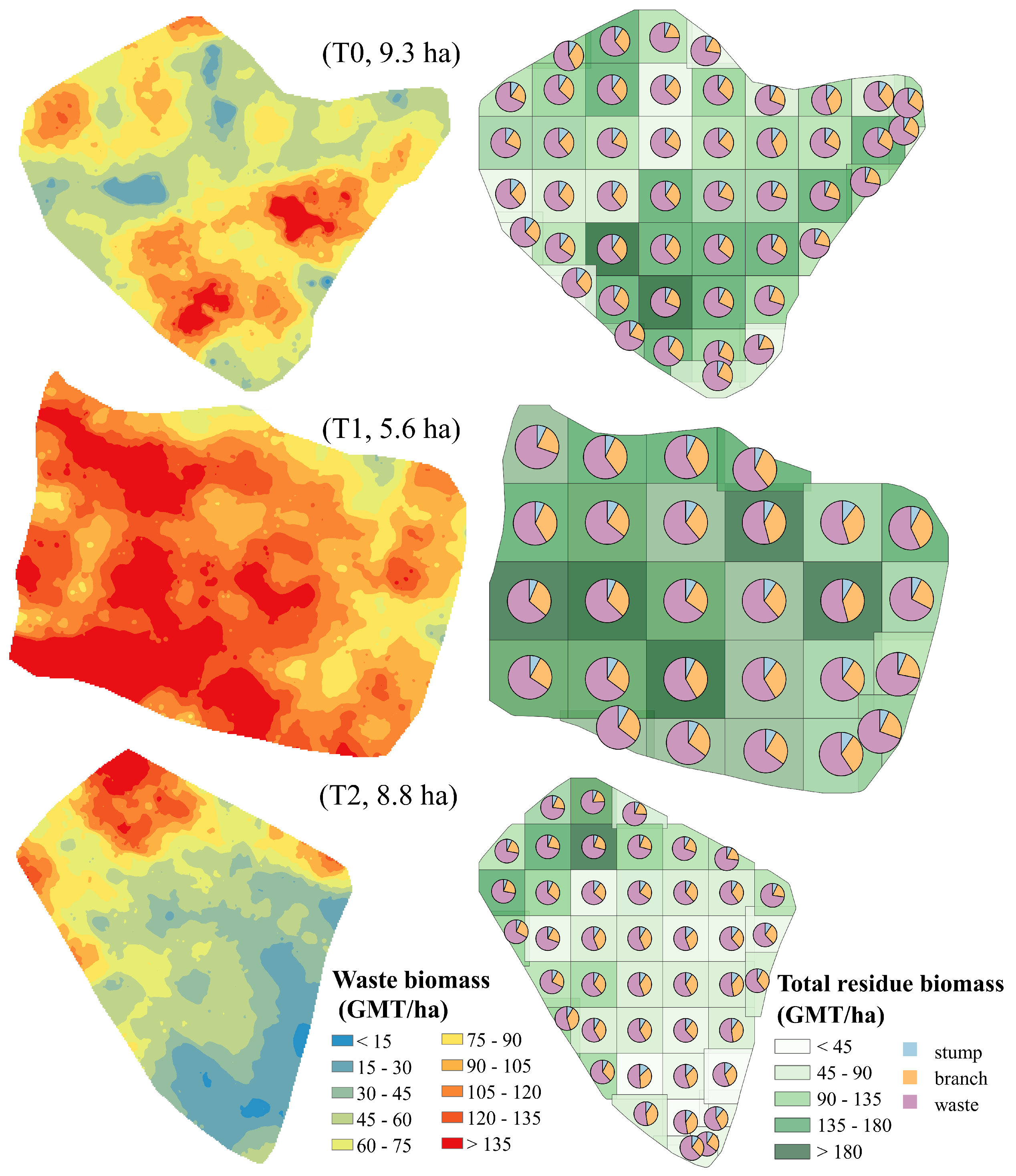
6.2. Estimates and Spatial Maps of Residue Biomass

The three approaches resulted in similar estimates for the branch and stump biomass but not for the waste and total residue biomass across the three stand types. The estimated branch biomass in green weight, when averaged over the grid cells, was in the range of 23.2–23.6, 52.7–55.8, and 28.5–30.5 t/ha among the three methods for the T0, T1, and T2 plantations. The corresponding dry weight ranges were 9.8–9.9, 17.2–17.9, and 11.1–11.6 t/ha for the T0, T1, and T2 plantations, respectively (Figure 7). The average stump biomass estimates in green weight were in the range of 6.7–7.9, 11.0–12.1, and 5.3–7.2 t/ha among the three methods for the T0, T1, and T2 plantations. The corresponding dry weight ranges were 4.1–4.5, 5.6–5.7, and 3.7–3.9 t/ha among the three methods. The highest estimates of waste biomass came from the third method, while the other two methods resulted in lower estimates. The waste biomass estimates obtained through the third method, when averaged over the grid cells, were 65.2, 88.5, and 60.2 t/ha in green weight and 34.1, 39.5, and 28.0 t/ha in dry weight for the T0, T1, and T2 plantations. The average waste biomass estimates obtained through the first and second methods were 35.1 and 32.7, 49.8 and 47.9, and 31.0 and 22.4 t/ha in green weight, and 17.4 and 15.3, 20.0 and 19.3, and 14.4 and 9.7 t/ha in dry weight for the T0, T1, and T2 plantations. These estimates of the waste biomass were 44–63% lower in comparison to those obtained through the third method (Figure 7).

The total residue biomass estimated through the third method, when averaged over the grid cells, was 96.7, 156.4, and 97.9 t/ha in green weight and 48.6, 63.0, and 43.5 t/ha in dry weight for the T0, T1, and T2 plantations (Figure 8,

Table 1. Estimates of total aboveground stand biomass (Total), total residue biomass (Residue), and its proportional allocation to the three residue components in green and dry weight that were obtained through each of the three methods (M) for the three stand types when averaged over grid cells.

Stand Type	Grid Cells	M	Green Weight					Dry Weight
			Total (t/ha)	Residue (t/ha)	Stump (%)	Waste (%)	Branch (%)	Total (t/ha)	Residue (t/ha)	Stump (%)	Waste (%)	Branch (%)
T0	254	1	387.8	66.0	10.9	53.9	35.2	205.4	31.4	13.1	55.7	31.2
		2	386.2	62.6	10.9	52.8	36.3	204.3	29.3	14.4	52	33.6
		3	364.0	96.7	8.2	67.7	24.1	188.6	48.6	9.4	70.3	20.3
T1	247	1	604.1	117.6	10.3	42.2	47.5	265.1	43.5	13.0	45.8	41.3
		2	609.4	111.6	10.1	43.4	46.6	267.1	42.1	13.4	45.9	40.7
		3	611.4	156.4	7.8	56.0	36.1	266.1	63.0	9.1	62.0	28.9
T2	203	1	420.8	68.8	10.5	45.3	44.2	196.9	29.8	13.1	48.2	38.7
		2	417.4	56.2	9.5	40.2	50.3	194.8	24.4	15.1	39.8	45.2
		3	425.8	97.9	8.1	58.5	33.5	196.0	43.5	9.9	61.3	28.9

). In comparison, the average estimates of the total residue biomass obtained through the first and second methods were 66.0 and 62.6, 117.6 and 111.6, and 68.8 and 56.2 t/ha in green weight, and 31.4 and 29.3, 43.5 and 42.1, and 29.8 and 24.4 t/ha in dry weight for the T0, T1, and T2 plantations. These estimates of the total residue biomass were 25–43% lower compared to those obtained through the third method (Figure 8). Among the three stand types, the total residue biomass estimates were the highest for T1 plantations. Waste biomass estimates comprised the greatest proportion of total residue biomass in T0 plantations regardless of the method of estimation. For the third method in particular, the estimated waste biomass in green weight accounted for 67.7% of the total residue biomass in T0 plantations, which was 11.7% and 9.2% higher than in T1 and T2 plantations (Table 1). The total and component residue biomass varied spatially within a harvest area and across stand types, as illustrated by the heatmaps and grid cell maps for the three example harvest areas in Figure 9.

6.3. Accuracy of Residue Biomass Estimation through Indirect Validation

The benchmarking statistics of indirect validation for all the stand types combined showed small and negligible biases in the residue biomass estimates obtained through the first method (

Table 2. Benchmarking statistics for the three methods of residue biomass estimation for all stand types combined.

	Fresh Weight					Dry Weight
	MEE (t/ha)	MPEE (%)	MAEE (t/ha)	MSEE	${\mathit{R}}_{\mathit{E}}^2$	MEE (t/ha)	MPEE (%)	MAEE (t/ha)	MSEE	${\mathit{R}}_{\mathit{E}}^2$
	M1
total	0.79	0.11	12.23	358.95	0.98	2.99	0.99	7.42	119.74	0.99
residue	−3.22	−2.53	10.97	190.34	0.88	−0.45	−1.11	4.96	41.14	0.91
stump	−0.58	−3.23	2.03	6.56	0.78	−0.34	−4.08	0.40	0.27	0.91
waste	−1.41	−1.75	8.72	119.46	0.85	0.25	0.49	4.75	38.89	0.86
branch	−1.53	−2.6	2.71	10.25	0.91	−0.33	−1.81	0.64	0.56	0.96
	M2
total	0.06	0.02	8.03	130.23	0.99	0.08	0.02	4.36	38.71	1.00
residue	0.17	0.42	9.24	137.96	0.91	0.13	0.47	4.25	32.58	0.93
stump	0.04	1.00	1.65	4.48	0.85	0.01	0.15	0.17	0.05	0.98
waste	0.09	0.72	7.21	86.00	0.89	0.12	1.20	4.02	29.14	0.89
branch	0.03	0.12	1.38	3.41	0.97	−0.00	0.02	0.35	0.22	0.98
	M3
total	29.24	4.84	42.83	3030.59	0.87	18.03	5.80	23.43	902.61	0.89
residue	−67.69	−30.26	68.32	7279.76	−3.71	−34.84	−34.45	34.96	1860.37	−3.23
stump	−0.58	−3.23	2.03	6.56	0.78	−0.34	−4.08	0.40	0.27	0.91
waste	−68.81	−44.94	69.31	7683.04	−8.73	−37.08	−48.65	37.24	2199.26	−7.17
branch	−1.53	−2.6	2.71	10.25	0.91	−0.33	−1.81	0.64	0.56	0.96

). The mean error of estimation (MEE) in dry weight was −0.45 t/ha (i.e., a slight overestimation) for the total residue biomass and fell within ±0.35 t/ha for the stump, waste, and branch biomass. The MEE values in fresh weight showed a slightly larger overestimation, but still less than 3.3% for all residue components as indicated by the values of the mean percentage error of estimation (MPEE). The average size of estimation error, as shown by the mean absolute error of estimation (MAEE), varied between 0.40 and 4.75 t/ha in dry weight and between 2.0 and 8.7 t/ha in fresh weight for the three residue components. The Nash–Sutcliffe coefficient of estimation efficiency ($R_E^2$) ranged between 0.86 and 0.96 for the residue components in dry weight, and between 0.78 and 0.91 in fresh weight. The benchmarking statistics for the second method indicated little bias and high precision in the estimation of all biomass components in both dry and fresh weight. The values of MAEE and MSEE were the smallest among the three methods. In comparison to the first two methods, the third method produced more waste biomass and consequently greater quantities of total residue biomass. The MEE values in fresh and dry weight were −68.8 and −37.1 t/ha for waste biomass and were −67.7 and −34.8 t/ha for total residue biomass. The corresponding $R_E^2$ values were all negative (Table 2).

The benchmarking statistics for the individual stand types showed that the first method had a slight underestimation of total residue biomass in dry weight of 0.31 and 1.2 t/ha for T0 and T1 stands, respectively, but an overestimation of 3.7 t/ha for T2 stands (Figure 10). The MEE values for waste biomass in dry weight was 1.1, 1.6, and −2.9 t/ha for T0, T1, and T2 stands, while the corresponding MPEE values were 2.6%, 10.6%, and −14.0%, respectively. The second method again showed the least bias and highest precision among the three methods in the estimation of all biomass components in both dry and fresh weight as indicated by the benchmarking statistics (Figure 10). In comparison to the first two methods, the third method produced greater amounts of waste biomass across the three stand types, with the MEE values being −79.5, −21.8, and −93.8 t/ha in fresh weight and −45.3, −11.6, and −45.7 t/ha for T0, T1, and T2 stands. The corresponding MPEE values in fresh as well as dry weight fell between −68.6% and −26.3% across the three stand types (Figure 10).

7. Discussion

Among the three methods of residue biomass estimation used in harvester data analytics, the first method provided the easiest and most straightforward link to the integration of harvester data with biomass equations. The DBHOB and total tree height of harvested stems are the only variables to be estimated from harvester data for the estimation of their residue biomass. This method could be easily implemented in a software tool, such as that developed by Woo et al. [38] for real-time monitoring and mapping of residue biomass during or soon after harvesting operations. However, this method cannot take into account the biomass in standing dead trees as they were usually fallen for safety reasons—if not knocked over by harvesting of surrounding trees—but not processed through the harvester head and thus were not contained in the harvester data. The biomass in standing dead trees could be a substantial part of the total residue biomass in unthinned plantations, particularly in areas with heavy self-thinning, drought induced mortality, or wind damage (e.g., [22,67,68]). If this biomass is left unaccounted for, the total residue biomass will be underestimated.

Unlike the first method, which relies on tree-level variables for residue biomass estimation, the second method was more involved as it required the stand-level attributes to be derived first from rasterised or gridded harvester data within a GIS system. The size of the grid cells would have to be determined first by considering (1) the stand density and its local-scale variations within plantations of different stand types that were present in the harvester data and (2) the extent of positional errors of the georeferenced stems. A grid of 50 m × 50 m was overlaid onto the harvester data in this study. Too small a grid cell size would result in the derived stand-level attributes varying outside of the applicable ranges of the stand-level biomass equations developed by Qiao et al. [23]. On the other hand, a very large cell size would smooth over local-scale variations in the estimated weight of residue biomass. Besides the grid size, whether to include partial grid cells along the boundary of a delineated forest area deserves careful consideration. In some other studies, grid cells more than half or fully within the delineated forest area were included in the analysis [44,46,55]. In this study, all grid cells, no matter full or partial, were included in the calculation of the stand-level attributes. The calculated density, basal area, and stand height were lower on average for the partial than for the full grid cells for all three stand types. These differences were likely due to the inclusion of 7 m buffer strips around the perimeter of the initially delineated plantation area (Figure 1). They also explained the slightly lower estimates of residue biomass than that obtained through the first method, as shown in Table 1. Therefore, buffer width presented a further factor to be considered when applying stand-level biomass equations to gridded harvester data. As all these issues in the gridding of the harvester data and the data analytics thereafter need to be resolved within a GIS system, this second method cannot be easily implemented in a software application for real-time stem-by-stem processing and analysis of the harvester data.

The third method was similar to but more refined than the first method and the refinement provided the most realistic and reliable estimates of waste biomass. The feature of this method lies in its more intensive use of harvester data in estimating the biomass of waste and offcut sections. Harvester recorded waste volumes were converted to biomass for individual trees using purposely derived conversion factors. For stems with a SEDTL greater than 8 cm, the specified minimum SEDOB for a pulp log, an offcut stem section above the top log that was not processed through the harvester head, was accounted for in the calculation of waste biomass. The volume of this unprocessed stem section was calculated using a taper function and converted to biomass using the same conversion factors. This approach of estimating waste biomass overcame certain limitations of the existing residue biomass equations of Wang et al. [29] and Qiao et al. [23] that were based on a finite number of sample trees. The samples included 59 trees from unthinned stands and 90 trees for each of the two thinned stand types. Although the sample size of 239 trees was relatively large in the parlance of the literature on biomass equations, the cutting patterns of this finite number of sample trees could not fully represent all actual cutting patterns of the large and almost infinite number of bucked stems captured by harvesters. Another limitation arose from the fact that the sample trees for developing biomass equations were usually selected to represent normal stems, while trees with malforms, defects, damages, or other anomalies were avoided. These trees would produce more and/or longer waste sections and greater waste volumes than similar sized trees with normal stems. Their stems were more likely not to be processed right through the harvester head up to the specified minimum SEDOB for commercial logs, as in the case of normal stems. Therefore, their recorded SEDTL would be far greater than the specified minimum SEDOB. The SEDTL distribution of stems contained in the harvester data had a much wider range than that of biomass sample trees, with a median of 13.5 cm, an upper quartile of 17.3 cm, and a 95th percentile of 28.7 cm. These distributional characteristics highlighted the necessity of including the unprocessed stem tops in the calculation of residue biomass for a substantial proportion of the harvested stems. Although the third method was more complicated than the first, it can still be implemented in a software application for real-time stem-by-stem processing and analysis of the harvester data. However, the estimated stump and waste biomass for T0 plantations would have to be adjusted to account for standing dead trees at stand level.

Due to the expanse of routine harvesting operations and the spatial scale of harvester data analytics, it was difficult to obtain in situ data for residue biomass to validate the calculated and spatially mapped residue biomass in the harvested plantations. To overcome this difficulty, this study tried indirect validation through ex-situ sample plots previously established in rotation-age P. radiata stands in the same study area. Although the benchmark statistics of indirect validation were informative and reassuring to a certain extent, they must be understood and interpreted with a clear understanding of the context and limitations of such indirect validation. Firstly, the sample plots and their matching virtual plots, albeit mostly similar in key stand attributes, might still differ somewhat in diameter and height distributions, in the stem from and branch architecture of individual trees, in site and stand conditions, and in the history of natural disturbances. Differences in these factors would also lead to the sample and the matching virtual plots having different quantities of residue biomass, thereby confounding, to a certain extent, the ‘error of estimation’ $\epsilon$ as calculated in Equation (4). Secondly, when residue biomass was estimated through the first two methods, i.e., using individual tree and stand-level biomass equations, an unstated implicit assumption was that the trees in the sample and the virtual plots had the same or similar cutting patterns. Consequently, the benchmarking statistics for the first two methods looked far better than those for the third method (Table 2, Figure 10). In the case of the second method, where stand-level biomass equations were used, the calculated residue biomass for a virtual plot was $M_V=f\left(N_V, G_V, H_V, A_V \right)$. When this relationship is substituted into Equation (4), the adjusted difference between $M_S$ and $M_V$ becomes $\epsilon =M_S-f\left(N_S, G_S, H_S, A_S \right)$, i.e., the prediction error of the biomass equation. Therefore, the benchmark statistics would reflect the predictive performance of the biomass equations over the sample data. In comparison to the first two methods, the third method reflected the real cutting patterns of stems in the virtual plots and generated a greater amount of waste biomass than the sample plots. Although the most realistic, this method had the worst benchmarking statistics (Table 2, Figure 10). The two contrasting interpretations highlighted the limitations of such indirect validation through ex-situ sample plots. Future validation studies are being planned at larger operational scales in another plantation area where log production and residue biomass recovery are integrated into plantation harvesting.

The estimates of total residue biomass obtained using the three methods through harvester data analytics varied between 56.2 and 156.4 t/ha in green weight across the three stand types in this study. These estimates were comparable to the quantities of residue biomass assessed using conventional sample plots, transects, or small blocks following CTL harvesting of rotation age P. radiata plantations elsewhere in Australia [22,28,69]. These quantities largely fell within the range of 50–150 GMT (Green Metric Tonnes)/ha, with an average that was slightly higher than 100 GMT/ha, except for one case study in a southern Tasmania plantation where an exceptionally high level of 238.6 GMT/ha was left after CTL harvesting [12]. However, there were differences between our estimates and the previously reported quantities of residue biomass. Firstly, stumps were not assessed and included as harvest residues in those previous studies. Although not a major residue component, stump biomass would account for 8–11% of the total residue biomass in green weight, as shown in Table 1. Secondly, the harvest residues in the previous studies were not always assessed at the time of harvesting, but 3–4 months following harvesting (e.g., [28,69]). Over this time, harvest residues could lose between 10% and 25% of their moisture depending on the season of harvesting, according to the natural drying curves for P. radiata shown in Strandgard et al. [13]. If this loss of moisture content were accounted for, some of the previously reported green weight quantities would have been at least 10% greater.

The conventional approach of assessing harvest residues through sample plots, transects, or small study blocks has provided site-specific estimates of residue biomass. For example, Strandgard and Mitchell [22] set up a study block of approximately 3 ha in a 29-year-old P. radiata plantation in Western Australia and found 104 GMT/ha of harvest residue biomass—not including stumps—following harvesting through the conventional CTL method that used a harvester-processor to fell/process and a forwarder to extract. This plantation had been thinned once at age 15 years and had subsequently suffered sporadic windthrow over approximately 80% of its area. Walsh et al. [69] assessed a 100-tree plot of approximately 0.5 ha in a 34-year-old T2 plantation of P. radiata near Tumut in NSW. The stand was high-yielding with trees of good form and quality, for which the total residue biomass was found to be 151 GMT/ha following CTL harvesting—about 24.3% of the total aboveground stand biomass not including stumps. Although such site-specific assessments of harvest residue biomass were informative, they could not be readily extrapolated over the plantation landscape to examine how harvest residue biomass and its components would vary with different thinning regimes and site and stand conditions. This limitation of the conventional approach can be easily overcome through harvester data analytics as demonstrated in this study.

Furthermore, the estimated residue biomass from harvester data analytics can be easily mapped for all residue components individually to reveal their spatial variation at different spatial scales. Such maps will assist operational planning of biomass recovery, particularly when residue harvesting is run as a separate operation. They will also assist in understanding the spatial variation of available residue biomass and in refining preharvest predictions of residue biomass that are based on LiDAR and inventory metrics when planning for integrated log harvesting and residue biomass recovery. For both types of operations, these maps will provide the basis for estimating site-specific nutrient removal for the composition and rate of the planned residue biomass recovery. A good understanding of biomass and nutrient pools at harvest and the impact of any planned residue biomass recovery on these pools is essential to maintain site productivity and nutrient balance in site-specific management for the long-term sustainability of P. radiata plantations (see [70,71,72,73]).

8. Conclusions

Pinus radiata plantations are a major source of harvest residue biomass for renewable bioenergy production in Australia. The utilization of this resource requires reliable assessments and estimation of the quantity and quality of residue biomass available for collection in rotation-age plantations over large geographical areas across the southern half of the Australian continent. This study demonstrated a novel approach through harvester data analytics to estimate and spatially map harvest residue biomass in plantations following CTL harvesting. Three methods of integrating biomass equations with harvester data at the tree and stand level were employed and compared for the estimation of stump, waste, branch, and total residue biomass in harvested plantations of three stand types: unthinned (T0), thinned once (T1), and thinned twice (T2). The estimates of total residue biomass obtained using the three methods varied between 56.2 and 156.4 t/ha in green weight and between 24.4 and 63.0 t/ha in dry weight across the three stand types. Among the three methods of residue biomass estimation employed in the harvester data analytics, the third method made the most intensive use of harvester data, relied on the cutting patterns of stems in routine harvesting, and thus provided more realistic estimates of waste biomass. The spatial mapping of the estimated total and component residue biomass will assist operational planning of biomass recovery for bioenergy production and site-specific nutrient management to ensure the long-term sustainability of P. radiata plantations.

References

1. Hall, J.P. Sustainable production of forest biomass for energy. For. Chron. 2002, 78, 391–396. [Google Scholar] [CrossRef] [Green Version]
2. Sims, R.E. Bioenergy to mitigate for climate change and meet the needs of society, the economy and the environment. Mitig. Adapt. Strateg. Glob. Chang. 2003, 8, 349–370. [Google Scholar] [CrossRef]
3. Acuña, E.; Cancino, J.; Rubilar, R.; Silva, L. Volume, physical characteristics and costs of harvest residue utilization of Pinus radiata as an energy source. Custos Agronegócio 2017, 13, 442–463. [Google Scholar]
4. Han, H.-S.; Jacobson, A.; Bilek, E.T.; Sessions, J. Waste to Wisdom: Utilizing forest residues for the production of bioenergy and biobased products. Appl. Eng. Agric. 2018, 34, 5–10. [Google Scholar] [CrossRef]
5. Campbell, R.M.; Anderson, N.M. Comprehensive comparative economic evaluation of woody biomass energy from silvicultural fuel treatments. J. Environ. Manag. 2019, 250, 109422. [Google Scholar] [CrossRef]
6. Hanssen, S.V.; Daioglou, V.; Steinmann, Z.J.; Frank, S.; Popp, A.; Brunelle, T.; Lauri, P.; Hasegawa, T.; Huijbregts, M.A.; Van Vuuren, D.P. Biomass residues as twenty-first century bioenergy feedstock—A comparison of eight integrated assessment models. Clim. Chang. 2020, 163, 1569–1586. [Google Scholar] [CrossRef] [Green Version]
7. Liu, W.; Hou, Y.; Liu, W.; Yang, M.; Yan, Y.; Peng, C.; Yu, Z. Global estimation of the climate change impact of logging residue utilization for biofuels. For. Ecol. Manag. 2020, 462, 118000. [Google Scholar] [CrossRef]
8. Van Holsbeeck, S.; Brown, M.; Srivastava, S.K.; Ghaffariyan, M.R. A Review on the Potential of Forest Biomass for Bioenergy in Australia. Energies 2020, 13, 1147. [Google Scholar] [CrossRef] [Green Version]
9. Kallio, A.M.I. Wood-based textile fibre market as part of the global forest-based bioeconomy. For. Policy Econ. 2021, 123, 102364. [Google Scholar] [CrossRef]
10. Titus, B.D.; Brown, K.; Helmisaari, H.-S.; Vanguelova, E.; Stupak, I.; Evans, A.; Clarke, N.; Guidi, C.; Bruckman, V.J.; Varnagiryte-Kabasinskiene, I. Sustainable forest biomass: A review of current residue harvesting guidelines. Energy Sustain. Soc. 2021, 11, 10. [Google Scholar] [CrossRef]
11. Spinelli, R.; Visser, R.; Björheden, R.; Röser, D. Recovering energy biomass in conventional forest operations: A review of integrated harvesting systems. Curr. For. Rep. 2019, 5, 90–100. [Google Scholar] [CrossRef]
12. Ghaffariyan, M.R.; Dupuis, É. Analyzing the impacts of harvesting methods on the quantity of harvest residues: An Australian case study. Forests 2021, 12, 1212. [Google Scholar] [CrossRef]
13. Strandgard, M.; Acuna, M.; Turner, P.; Mirowski, L. Use of modelling to compare the impact of roadside drying of Pinus radiata D.Don logs and logging residues on delivered costs using high capacity trucks in Australia. Biomass Bioenergy 2021, 147, 106000. [Google Scholar] [CrossRef]
14. Ghaffariyan, M.R. Remaining slash in different harvesting operation sites in Australian plantations. Silva Balc. 2013, 14, 83–93. [Google Scholar]
15. Ghaffariyan, M.R.; Apolit, R. Harvest residues assessment in pine plantations harvested by whole tree and cut-to-length harvesting methods (A case study in Queensland, Australia). Silva Balc. 2015, 16, 113–122. [Google Scholar]
16. Laitila, J.; Asikainen, A.; Hotari, S. Residue recovery and site preparation in a single operation in regeneration areas. Biomass Bioenergy 2005, 28, 161–169. [Google Scholar] [CrossRef]
17. Berry, M.; Sessions, J. Evaluating the Economic Incentives of Biomass Removal on Site Preparation for Different Harvesting Systems in Australia. Forests 2020, 11, 1370. [Google Scholar] [CrossRef]
18. Mead, D.J. Sustainable Management of Pinus Radiata Plantations; Food and Agriculture Organization of the United Nations (FAO): Rome, Italy, 2013; p. 264. [Google Scholar]
19. Burdon, R.; Libby, W.; Brown, A. Domestication of Radiata Pine; Springer: Berlin/Heidelberg, Germany, 2017; Volume 83. [Google Scholar]
20. Downham, R.; Gavran, M. Australian Plantation Statistics 2020 Update. 2020. Available online: https://www.awe.gov.au/abares/research-topics/forests/forest-economics/plantation-and-log-supply (accessed on 15 July 2021).
21. Smethurst, P.J.; Nambiar, E.K.S. Distribution of carbon and nutrients and fluxes of mineral nitrogen after clear-felling a Pinus radiata plantation. Can. J. For. Res. 1990, 20, 1490–1497. [Google Scholar] [CrossRef]
22. Strandgard, M.; Mitchell, R. Comparison of cost, productivity and residue yield of cut-to-length and fuel-adapted harvesting in a Pinus radiata D. Don final harvest in Western Australia. N. Z. J. For. Sci. 2019, 49, 12. [Google Scholar] [CrossRef] [Green Version]
23. Qiao, X.; Bi, H.; Li, Y.; Ximenes, F.; Weston, C.J.; Volkova, L.; Ghaffariyan, M.R. Additive predictions of aboveground stand biomass in commercial logs and harvest residues for rotation age Pinus radiata plantations in New South Wales, Australia. J. For. Res. 2021, 32, 2265–2289. [Google Scholar] [CrossRef]
24. Ghaffariyan, M.R.; Brown, M.; Acuna, M.; Sessions, J.; Gallagher, T.; Kühmaier, M.; Spinelli, R.; Visser, R.; Devlin, G.; Eliasson, L.; et al. An international review of the most productive and cost-effective forest biomass recovery technologies and supply chains. Renew. Sustain. Energy Rev. 2017, 74, 145–158. [Google Scholar] [CrossRef]
25. Lock, P.; Whittle, L. Future Opportunities for Using Forest and Sawmill Residues in Australia; Australian Bureau of Agricultural and Resource Economics and Sciences (ABARES): Canberra, Australia, 2018; p. 83.
26. Ghaffariyan, M.R.; Acuna, M.; Brown, M. Analysing the effect of five operational factors on forest residue supply chain costs: A case study in Western Australia. Biomass Bioenergy 2013, 59, 486–493. [Google Scholar] [CrossRef]
27. Zamora-Cristales, R.; Sessions, J. Modeling harvest forest residue collection for bioenergy production. Croat. J. For. Eng. J. Theory Appl. For. Eng. 2016, 37, 287–296. [Google Scholar]
28. Ghaffariyan, M.R.; Sessions, J.; Brown, M.W. Collecting harvesting residues in pine plantations using a mobile chipper in Victoria (Australia). Silva Balc. 2014, 15, 81–95. [Google Scholar]
29. Wang, X.; Bi, H.; Ximenes, F.; Ramos, J.; Li, Y. Product and Residue Biomass Equations for Individual Trees in Rotation Age Pinus radiata Stands under Three Thinning Regimes in New South Wales, Australia. Forests 2017, 8, 439. [Google Scholar] [CrossRef] [Green Version]
30. Ghaffariyan, M.R.; Sessions, J.; Brown, M.W. Evaluating productivity, cost, chip quality and biomass recovery for a mobile chipper in Australian roadside chipping operations. J. For. Sci. 2012, 58, 530–535. [Google Scholar] [CrossRef] [Green Version]
31. Ghaffariyan, M.R.; Spinelli, R.; Magagnotti, N.; Brown, M. Integrated harvesting for conventional log and energy wood assortments: A case study in a pine plantation in Western Australia. South. For. J. For. Sci. 2015, 77, 249–254. [Google Scholar] [CrossRef]
32. Priddle, J. Computer-Controlled Optimisation in Cut-to-Length Harvesting Systems and Associated Data Flows. 2005. Available online: https://gottsteintrust.org/projects-reports/report/41-computer-controlled-optimisation-in-cut-to-length-harvesting-systems-and-associated-data-flows (accessed on 15 July 2021).
33. Skogforsk. StanForD 2010—Moderne Kommunikation mit Forstmaschinen. Available online: https://www.skogforsk.se/cd_20190114162016/contentassets/1a68cdce4af1462ead048b7a5ef1cc06/stanford-2010-german.pdf (accessed on 6 June 2021).
34. Kemmerer, J.; Labelle, E.R. Using harvester data from on-board computers: A review of key findings, opportunities and challenges. Eur. J. For. Res. 2020, 140, 1–17. [Google Scholar] [CrossRef]
35. Kiljunen, N. Estimating dry mass of logging residues from final cuttings using a harvester data management system. Int. J. For. Eng. 2002, 13, 17–25. [Google Scholar] [CrossRef]
36. Palander, T.; Vesa, L.; Tokola, T.; Pihlaja, P.; Ovaskainen, H. Modelling the stump biomass of stands for energy production using a harvester data management system. Biosyst. Eng. 2009, 102, 69–74. [Google Scholar] [CrossRef]
37. Vesa, L.; Palander, T. Modeling stump biomass of stands using harvester measurements for adaptive energy wood procurement systems. Energy 2010, 35, 3717–3721. [Google Scholar] [CrossRef]
38. Woo, H.; Acuna, M.; Choi, B.; Han, S.-K. FIELD: A Software Tool That Integrates Harvester Data and Allometric Equations for a Dynamic Estimation of Forest Harvesting Residues. Forests 2021, 12, 834. [Google Scholar] [CrossRef]
39. Snowdon, P.; Eamus, D.; Gibbons, P.; Keith, H.; Raison, J.; Kirschbaum, M. Synthesis of Allometrics, Review of Root Biomass, and Design of Future Woody Biomass Sampling Strategies; Australian Greenhouse Office: Canberra, Australia, 2000; p. 133.
40. Bi, H.; Long, Y.; Turner, J.; Lei, Y.; Snowdon, P.; Li, Y.; Harper, R.; Zerihun, A.; Ximenes, F. Additive prediction of aboveground biomass for Pinus radiata (D. Don) plantations. For. Ecol. Manag. 2010, 259, 2301–2314. [Google Scholar] [CrossRef]
41. Dupuis, É.; Ghaffariyan, M. Quantitative and qualitative analysis of harvesting residues in Australian plantations. In Proceedings of the ANZ Biochar Conference, Online, 16–17 July 2020. [Google Scholar]
42. Lu, K.; Bi, H.; Watt, D.; Strandgard, M.; Li, Y. Reconstructing the size of individual trees using log data from cut-to-length harvesters in Pinus radiata plantations: A case study in NSW, Australia. J. For. Res. 2018, 29, 13–33. [Google Scholar] [CrossRef] [Green Version]
43. Shan, C.; Bi, H.; Watt, D.; Li, Y.; Strandgard, M.; Ghaffariyan, M.R. A new model for predicting the total tree height for stems cut-to-length by harvesters in Pinus radiata plantations. J. For. Res. 2021, 32, 21–41. [Google Scholar] [CrossRef] [Green Version]
44. Rasinmäki, J.; Melkas, T. A method for estimating tree composition and volume using harvester data. Scand. J. For. Res. 2005, 20, 85–95. [Google Scholar] [CrossRef]
45. Bollandsås, O.M.; Maltamo, M.; Gobakken, T.; Lien, V.; Næssset, E. Prediction of Timber Quality Parameters of Forest Stands by Means of Small Footprint Airborne Laser Scanner Data. Int. J. For. Eng. 2011, 22, 14–23. [Google Scholar] [CrossRef]
46. Maltamo, M.; Hauglin, M.; Næsset, E.; Gobakken, T. Estimating stand level stem diameter distribution utilizing harvester data and airborne laser scanning. Silva Fenn. 2019, 53, 10075. [Google Scholar] [CrossRef]
47. Karjalainen, T.; Mehtätalo, L.; Packalen, P.; Gobakken, T.; Næsset, E.; Maltamo, M. Field calibration of merchantable and sawlog volumes in forest inventories based on airborne laser scanning. Can. J. For. Res. 2020, 50, 1352–1364. [Google Scholar] [CrossRef]
48. Knott, J.; Ryan, P. Development and Practical Application of a Soils Database for the Pinus Plantations of the Bathurst Region; Research Paper No. 11; Forestry Commission of New South Wales: Sydney, Australia, 1990; p. 85. [Google Scholar]
49. Anon. Forest Management Plan. Available online: https://www.forestrycorporation.com.au/__data/assets/pdf_file/0010/660628/forest-management-plan-softwood-plantations.pdf (accessed on 15 June 2021).
50. Skogforsk. Standard for Forest Data and Communications. 2007. Available online: https://www.skogforsk.se/contentassets/b063db555a664ff8b515ce121f4a42d1/stanford_maindoc_070327.pdf (accessed on 6 June 2021).
51. Arlinger, J.; Nordström, M.; Möller, J.J. StanForD 2010: Modern Communication with Forest Machines; Skogforsk: Uppsala, Sweden, 2012; Volume 785. [Google Scholar]
52. Lindroos, O.; Ringdahl, O.; La Hera, P.; Hohnloser, P.; Hellström, T.H. Estimating the position of the harvester head–a key step towards the precision forestry of the future? Croat. J. For. Eng. 2015, 36, 147–164. [Google Scholar]
53. Asaeedi, S.; Didehvar, F.; Mohades, A. α-Concave hull, a generalization of convex hull. Theor. Comput. Sci. 2017, 702, 48–59. [Google Scholar] [CrossRef]
54. Leech, J. Estimating crown width from diameter at breast height for open-grown radiata pine trees in South Australia. Aust. For. Res. 1984, 14, 333–337. [Google Scholar]
55. Hauglin, M.; Hansen, E.; Sørngård, E.; Næsset, E.; Gobakken, T. Utilizing accurately positioned harvester data: Modelling forest volume with airborne laser scanning. Can. J. For. Res. 2018, 48, 913–922. [Google Scholar] [CrossRef]
56. Söderberg, J.; Wallerman, J.; Almäng, A.; Möller, J.J.; Willén, E. Operational prediction of forest attributes using standardised harvester data and airborne laser scanning data in Sweden. Scand. J. For. Res. 2021, 36, 306–314. [Google Scholar] [CrossRef]
57. García, O. Estimating top height with variable plot sizes. Can. J. For. Res. 1998, 28, 1509–1517. [Google Scholar] [CrossRef]
58. García, O. Scale and spatial structure effects on tree size distributions: Implications for growth and yield modelling. Can. J. For. Res. 2006, 36, 2983–2993. [Google Scholar] [CrossRef] [Green Version]
59. Zhou, M.; Lei, X.; Duan, G.; Lu, J.; Zhang, H. The effect of the calculation method, plot size, and stand density on the top height estimation in natural spruce-fir-broadleaf mixed forests. For. Ecol. Manag. 2019, 453, 117574. [Google Scholar] [CrossRef]
60. Bi, H. Trigonometric variable-form taper equations for Australian eucalypts. For. Sci. 2000, 46, 397–409. [Google Scholar]
61. Nash, J.E.; Sutcliffe, J.V. River flow forecasting through conceptual models part I—A discussion of principles. J. Hydrol. 1970, 10, 282–290. [Google Scholar] [CrossRef]
62. Wackerly, D.; Mendenhall, W.; Scheaffer, R.L. Mathematical Statistics with Applications; Duxbury Press: London, UK, 1996; p. 329. [Google Scholar]
63. Loague, K.; Green, R.E. Statistical and graphical methods for evaluating solute transport models: Overview and application. J. Contam. Hydrol. 1991, 7, 51–73. [Google Scholar] [CrossRef]
64. Mayer, D.; Butler, D. Statistical validation. Ecol. Model. 1993, 68, 21–32. [Google Scholar] [CrossRef]
65. Vanclay, J.K. Modelling Forest Growth and Yield: Applications to Mixed Tropical Forests; CABI Publishing: Wallingford, UK, 1994; p. 336. [Google Scholar]
66. Huang, S.; Yang, Y.; Wang, Y. A critical look at procedures for validating growth and yield models. In Modelling Forest Systems; CABI Publishing: Oxford, UK, 2003; pp. 271–292. [Google Scholar]
67. Bi, H. The self-thinning surface. For. Sci. 2001, 47, 361–370. [Google Scholar]
68. Stone, C.; Penman, T.; Turner, R. Managing drought-induced mortality in Pinus radiata plantations under climate change conditions: A local approach using digital camera data. For. Ecol. Manag. 2012, 265, 94–101. [Google Scholar] [CrossRef]
69. Walsh, D.; Wiedemann, J.; Strandgard, M.; Ghaffariyan, M.R.; Skinnell, J. ‘FibrePlus’ Study: Harvesting Stemwood Waste Pieces in Pine Clearfall; Bulletin 18; CRC for Forestry: Tasmania, Australia, 2011. [Google Scholar]
70. Smith, C.; Lowe, A.; Skinner, M.; Beets, P.; Schoenholtz, S.; Fang, S. Response of radiata pine forests to residue management and fertilisation across a fertility gradient in New Zealand. For. Ecol. Manag. 2000, 138, 203–223. [Google Scholar] [CrossRef]
71. Turner, J.; Lambert, M.J.; Hopmans, P.; McGrath, J. Site variation in Pinus radiata plantations and implications for site specific management. New For. 2001, 21, 249–282. [Google Scholar] [CrossRef]
72. Garrett, L.; Beets, P.; Clinton, P.; Smaill, S. National series of long-term intensive harvesting trials in Pinus radiata stands in New Zealand: Initial biomass, carbon and nutrient pool data. Data Brief 2019, 27, 104757. [Google Scholar] [CrossRef]
73. Garrett, L.; Smith, C.; Beets, P.; Kimberley, M. Early rotation biomass and nutrient accumulation of Pinus radiata forests after harvest residue management and fertiliser treatment on contrasting types of soil. For. Ecol. Manag. 2021, 496, 119426. [Google Scholar] [CrossRef]
Figure 1. Distribution of harvested trees (dark green dots) within a delineated forest area. A buffer strip of 7 m was made around its perimeter and a grid of 50 m × 50 m was laid out over the area. The dot size reflects the estimated DBHOB of trees. Partial grid cells filled with light blue along the boundary were expanded at all sides (dark salmon strips) to contain at least 35 trees for the calculation of their stand attributes (see text).
Forests 13 00428 g001
Figure 2. Examples of sample plots (left) and their matching virtual plots (right) in unthinned (T0), thinned once (T1), and thinned twice (T2) stands. The radius of each pair of plots was shown in the sample plot. The solid dots indicate the spatial locations of live (green) and dead (red) trees, while dot size is proportional to DBHOB. Stand attributes of the three pairs of plots are shown in the central text column. The clustered patterns of trees in the virtual plots reflect the harvester recorded spatial locations of harvested stems.
Forests 13 00428 g002
Figure 3. Scatterplots of stand attributes for the sample plots in T0 (blue), T1 (brown), and T2 (green) stands against that of their matching virtual plots with a diagonal line of unity (top). Boxplots of relative differences in stand attributes between the sample and the virtual plots for the three stand types (bottom). Relative differences are expressed as the percentages of the sample plot values.
Forests 13 00428 g003
Figure 4. Boxplots of estimated DBHOB and total tree height for the bucked stems contained in the harvester data set for each of the three stand types. The number next to each boxplot on the right indicates the number of stems for the corresponding stand type.
Forests 13 00428 g004
Figure 5. Boxplots of estimated stand-level attributes of individual grid cells for each of the three stand types. The number next to each boxplot on the right indicates the number of grid cells for the corresponding stand type.
Forests 13 00428 g005
Figure 6. Scatterplot matrix of stand-level attributes calculated for individual grid cells for the T0 (blue), T1 (brown), and T2 (green) plantations.
Forests 13 00428 g006
Figure 7. Boxplots of biomass estimates for three residue components in green and dry weight obtained through the three estimation methods for T0, T1, and T2 plantations.
Forests 13 00428 g007
Figure 8. Boxplots of total residue biomass estimates in green and dry weight obtained through the three estimation methods for T0, T1, and T2 plantations. The numbers on the right-hand side of the left graphic panel indicate the total number of grid cells for each of the three stand types.
Forests 13 00428 g008
Figure 9. Heatmaps of waste biomass in green weight for three harvested areas representing T0, T1, and T2 plantations (Left). Grid cell maps of total harvest residue biomass in green weight and its proportional allocation to the three residue components (Right). The biomass quantities were calculated using the third method through harvester data analytics.
Forests 13 00428 g009
Figure 10. Dot plots displaying five benchmarking statistics for indirect validation of residue biomass estimates in fresh and dry weight (upper and lower halves) that were obtained through harvester data analytics for three types of stands: unthinned (T0), thinned once (T1), and thinned twice (T2). Total residue biomass is labelled as ‘Residue’ in the yellow strip at the right end of each graph. M1, M2, and M3 in the legend represent the first, second, and third method of residue biomass calculation used in data analytics (see text). Due to space limitations, dot points showing R E 2 < 0 were indicative only, and do not represent the actual values.
Forests 13 00428 g010