2.1. Object of Study and Material
Forests in Poland occupied 29.6% of the country’s area in 2020 [
59]. Most of them were coniferous forests (68.2% of the total forest area), with pine
Pinus sylvestris L. dominating in species composition (58% of the total forest area). In the mid-1980s, it was estimated that there were about 26,000 forest patches in the state forests of Poland alone, which covered about 7 million ha [
60]. In 2006, about 50% of the forest area was considered fragmented by agricultural land or other artificial land [
37]. In 2020, there were 338,682 forest patches in Poland, of which only 37,443 (about 11%) had an area greater than 5 ha. However, the percentage of large forest patches (≥500 ha) was very high and amounted to about 85% of the total forest area in Poland [
61].
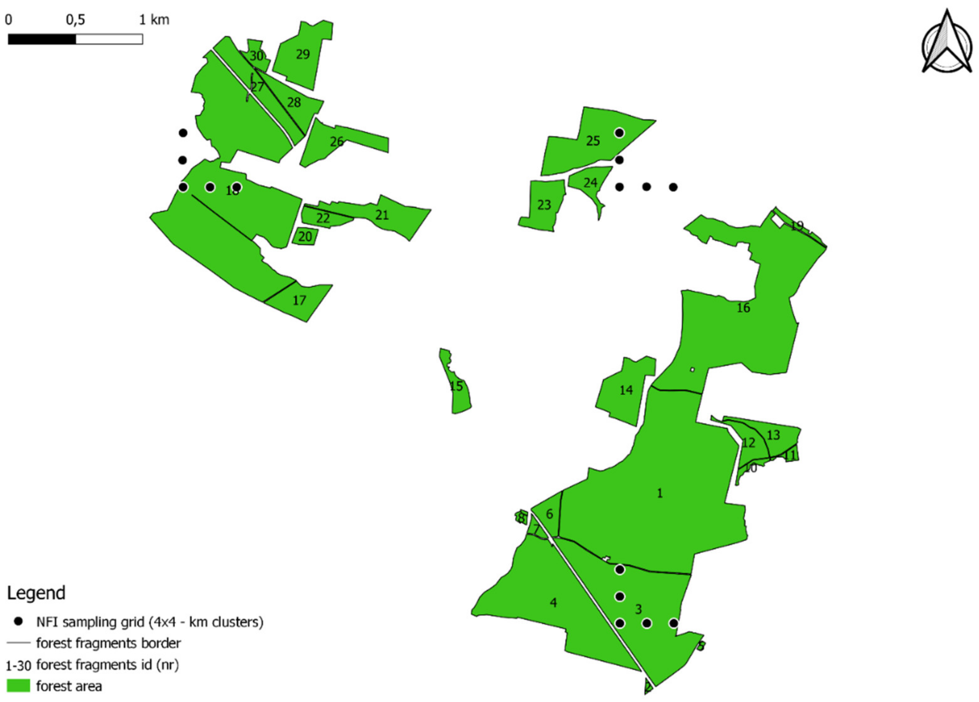
The research material consisted of data from field measurements of trees describing the condition of forests and data describing topographic objects in the country. The field data came from measurements made on National Forest Inventory (NFI) sample plots. The NFI system in Poland is a grid of sample plots grouped into clusters. The clusters are located in a 4 × 4 km grid. Each cluster has the shape of an L letter and consists of 5 permanent circular sample plots separated by a distance of 200 m (
Figure 1). According to the methodological assumptions, all living trees with a diameter at breast height of 70 mm or more are measured at regular intervals (5-year cycle) in each sample plot (constant area of 0.04 ha). Diameter at breast height is measured with an accuracy of 1 mm, and tree height is measured up to 1 dcm [
62].
Data from field measurements conducted during the third NFI cycle (years 2015–2019) were used for the analysis. Since the vast majority of forests in Poland are managed forests, areas under strict nature conservation were excluded from the analysis. Uniformly managed stands were selected as study material. Only NFI sample plots with tree canopy (stands) were considered. Plots without trees, e.g., temporarily unstocked due to clear-cutting as part of forest management, or those that were located along forest roads, were not included. Due to the small number, plots established in uneven-aged stands were also excluded from the analyses. To ensure homogeneity of the sample, plots established in the range of border between forest habitats that differed in fertility, humidity, species composition, age, vertical structure, or land use practices (management) were also excluded from the analyses. Based on these assumptions, of the total number of 35,342 plots listed in the 3rd cycle NFI database, the results of 20,381 plots were used for further analysis.
The Topographic Objects Database (TOD) was used to delineate forest patches. TOD is a vector database that contains the spatial location of topographic objects with their basic characteristics. Vector data representing 764,850 polygons described as forest fragments were used for the study.
2.2. Spatial Analysis and Database Analysis
The analytical work began with the integration of the NFI and TOD databases. The integration procedure consisted of three stages. In the first stage, the TOD vector data describing the forest fragments (
Figure 1) were generalized using QGIS software [
63]. The goal was to connect small polygons (forest fragments) into larger units (forest patches) based on structural connectivity. Forest patches were assumed to form adjacent forest fragments if the Euclidean distance between their boundaries was equal to or less than 50 m in at least one point. There are several reasons why we chose the criterion of 50 m. In the study by Ranta et al. [
25], the distance indicating isolation between forest fragments was not less than 50 m. This distance as a threshold for isolation is also confirmed by other authors [
64] who conducted their study in Poland. Such distance takes into account the assumptions for planned cuttings in managed forests that the clearcut area should be protected by the adjacent wall of a mature stand [
53]. Foresters have often applied a “rule of thumb” that the range of protection provided by a mature stand is equal to one tree’s height [
53]. Since the average height of mature stands in Poland is in the range of 25–35 m, the use of a distance of 50 m as a criterion for isolating patches seems to be correct (2 × 25 m, as the mutual distance between two forest fragments is analyzed). The last reason was that 50 m is the minimum width for expressways set by Polish law. The noise level and fences erected along such roads makes a significant barrier from this type of infrastructure. The minimum area of the forest patch was set at 0.01 hectares. As a result of spatial analyses, 764,850 forest fragments were combined into 401,045 forest patches. Among them, the largest forest patch had an area of 1377.5 thousand ha.
In the next phase, edge zones were distinguished in each forest patch. It was decided that the edge zone forms a 50 m wide strip of forest land extending from the boundary of the forest patch towards its interior. Such edge zone width value was chosen because, according to the literature studied [
14,
38,
41,
50,
51,
65,
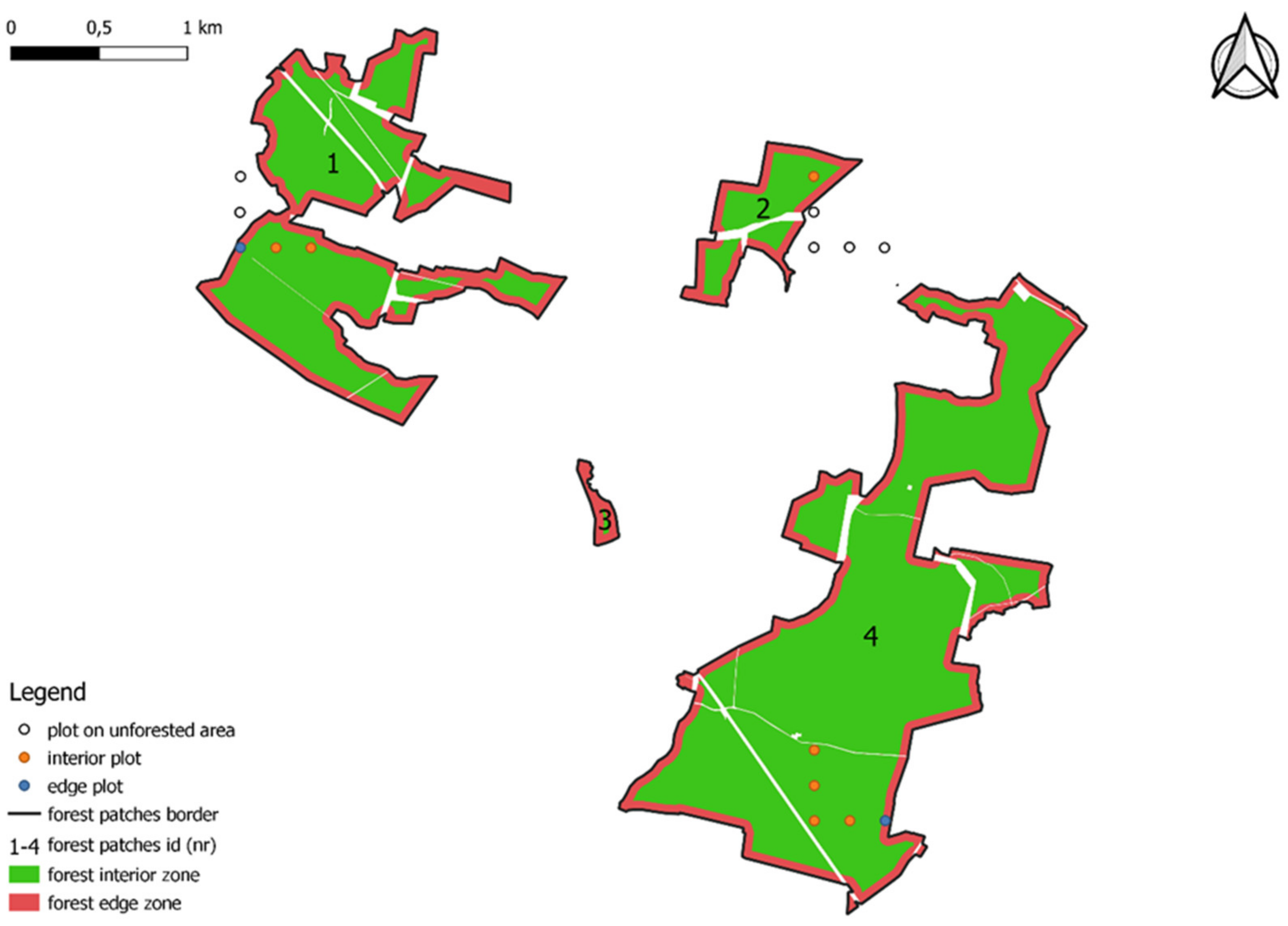
66], stands located up to 50 m from the forest margin usually are characterized by different structural parameters and microclimate conditions caused by edge effect. Only edge zones adjacent to the “open area” (matrix) were included in the study (
Figure 2). The “buffer” tool in QGIS was used to determine these zones [
63]. As a result of the spatial analyses along the boundaries of the forest patches and within the area of the forest fragments, an internal buffer of 50 m was determined. Then, the area of forest edge habitats and their percentage of the forest patch were calculated.
In the third phase, NFI plots were assigned to forest patches based on geographic coordinates, taking into account location: interior or edge zone (
Figure 2). As a result, 17,321 interior plots and 3060 edge plots were identified.
All tested plots (20,381) were distributed within 2906 forest patches.
To evaluate the volume of the wood resources, some criteria were established to filter sample plots. Only plots that were in a stand with a vertical structure of one, two or three canopy layers were used. Sample plots with residual trees, i.e., trees left over from the previous generation of the stand that have been left to die naturally, were omitted. All analyses of the volume and structure of wood resources in the interior and the edge zones of forest patches were the same and were performed for homogeneous computational units based on the grouping of plots in terms of:
Species composition—Plots were assigned the name of the dominant species (species with the highest growing stock volume on the plot);
Stand age—Each plot was assigned an age class number, determined by the age of the dominant species. The following age class rules were adopted: the age of the dominant species 1–10 years, 1 age class; the age of the dominant species 11–20 years, 2 age class, etc.;
Fertility and humidity of the habitat, based on the forest site type.
In this way, homogeneous computational units in terms of management, species composition, age, and habitat conditions were obtained. To ensure the reliability of the obtained results, only the computational units consisting of at least 100 sample plots were selected for further statistical analysis. Based on this procedure, 30 computational units described by a total of 9551 plots were distinguished from 20,381 plots.
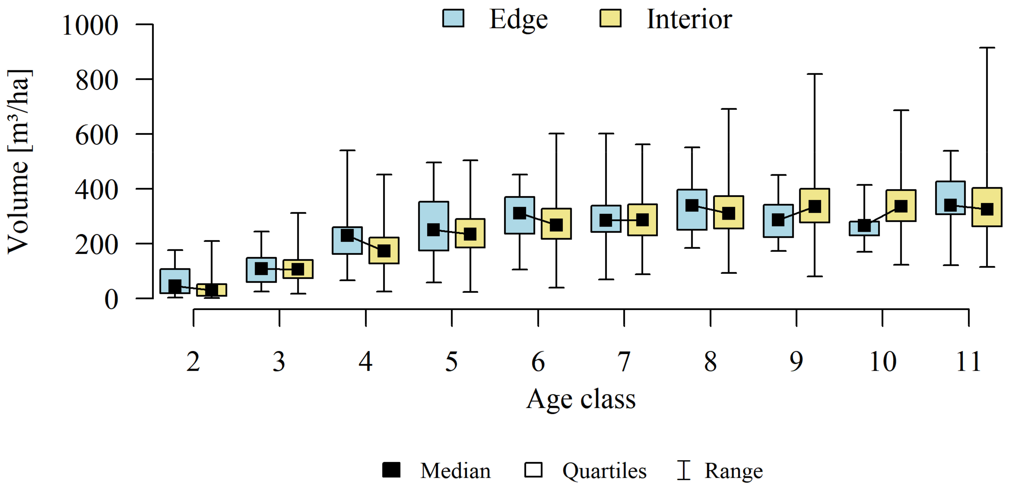
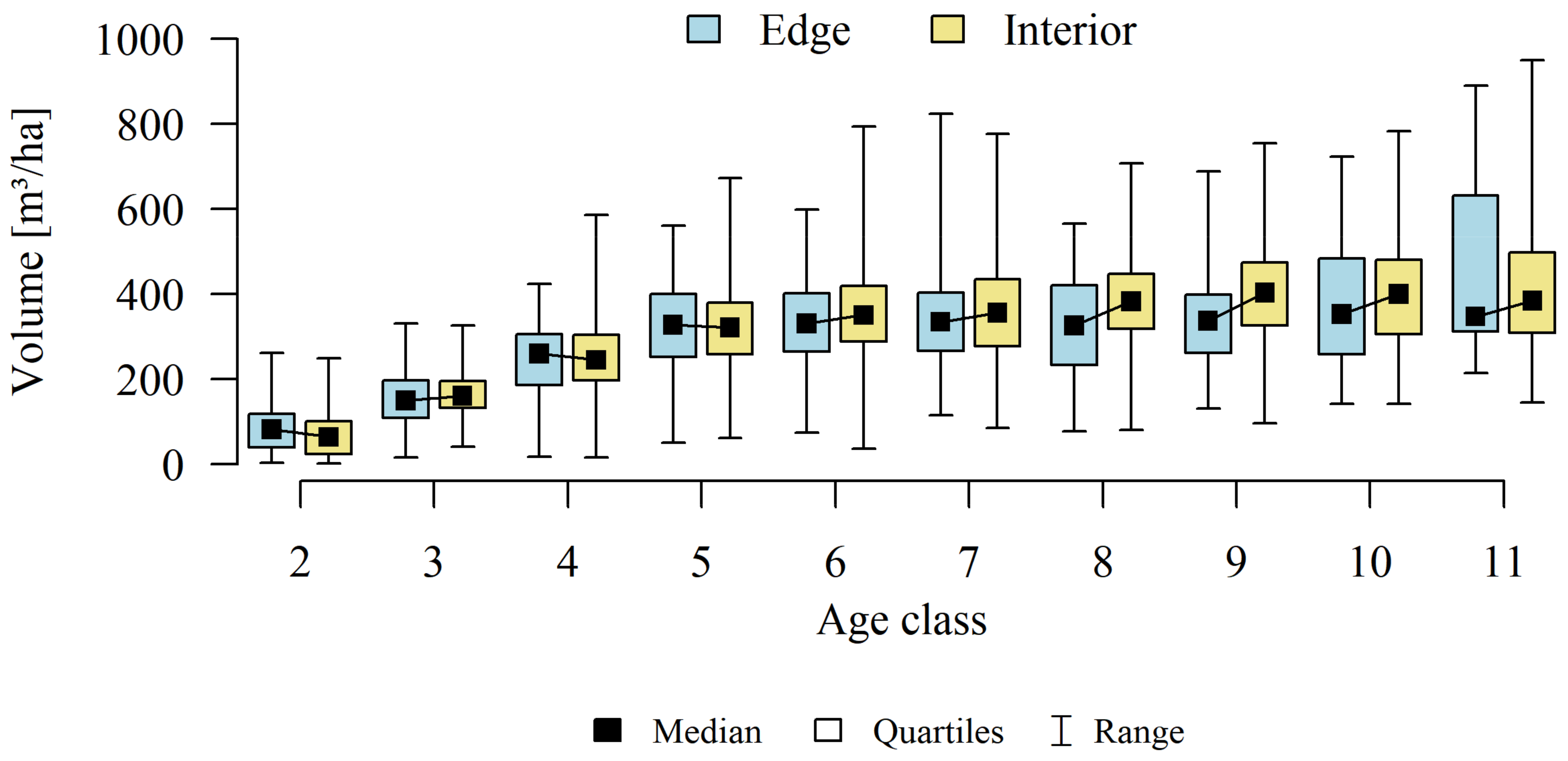
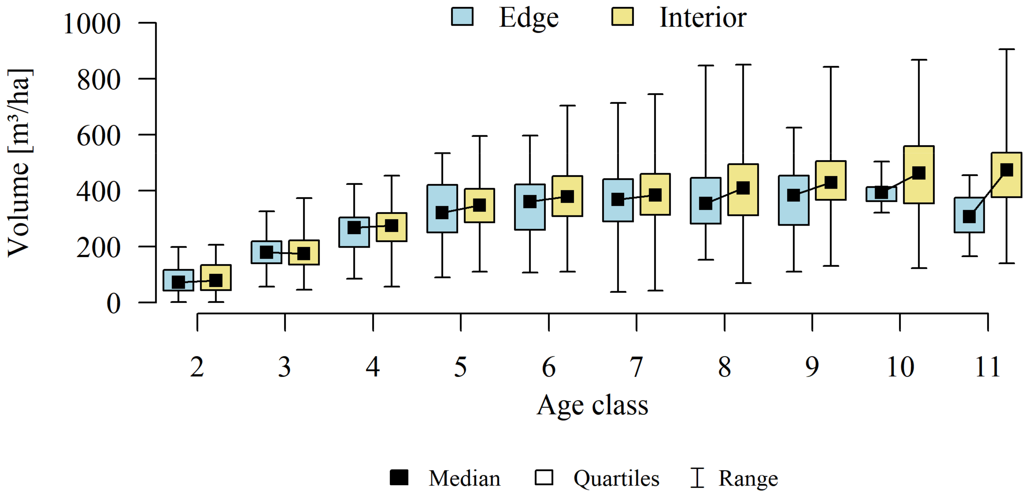
Analyses of the volume and structure of wood resources in the interior and edge zones of forest patches were conducted for stands with dominant pine in the 2 to 11 age classes in fresh coniferous forest (FCF—strongly barren habitat, fresh mixed coniferous forest (FMCF—barren habitat, and fresh mixed broadleaved forest (FMBF—moderately fertile habitat. For this purpose, the NFI database was used, from which the following characteristics were extracted for each sample plot: growing stock volume, growing stock volume increment, basal area.
2.3. Statistical Analysis and Calculations
Most statistical analyses were performed using the program R [
67]. For the evaluation of the volume and structure of wood resources in scientific studies of forest ecosystems, the most commonly used characteristics are basal area, growing stock volume, and growing stock increment. However, these characteristics are often interrelated. Therefore, before conducting further analyses, we assessed whether the sample plots were significantly correlated with respect to the listed characteristics. Spearman’s rank correlation was used to evaluate the interdependence of the studied characteristics.
The obtained results confirmed that there are statistically significant correlations between basal area (g), growing stock volume (v), and growing stock volume increment (zv) (
Table 1). Therefore, the studies selected one characteristic for further analysis of the volume and structure of wood resources-growing stock (v).
The study then focused on finding answers: whether there is a direct, statistically significant relationship between the relative volume of the resource (growing stock volume on plots) and the size of the forest patches (natural logarithm calculated from the area) and the proportion of the edge zone in the forest patches. A linear regression model and coefficient of determination (R2) were used.
As part of the adopted calculation procedure for each calculation unit, we investigated whether the wood resources in the interior and edge zones differ significantly. Considering that part of the observations (sample plots) are correlated with each other (plots established in the same forest patch), a mixed linear model was used to achieve the research objective. This means that the classical covariance matrix of the linear model was replaced by a matrix that allows correlations between observations.
The study of the significance of the differences between the resources in the interior of the patch and in its edge zones was carried out with a linear mixed model of the following form (Equation (1)):
where:
y–is the n data vector (dependent value),
X–is a matrix of n x p which columns are p independent variables that are permanent effects. In our calculations, X is the location of the plot in the forest patch (a variable taking two possible values: edge or interior),
β–is the p vector of permanent effects parameters,
Z–is a matrix of n x q which columns are q independent variables that are random effects. In our calculations, Z is the id of the forest patch (a qualitative variable denoting the identification code of the patch),
u–is the q vector of random effects parameters,
ε–is the n random vector.
Differences in growing stock volume between the interior and edge zones were considered significant for p ≤ 0.05.
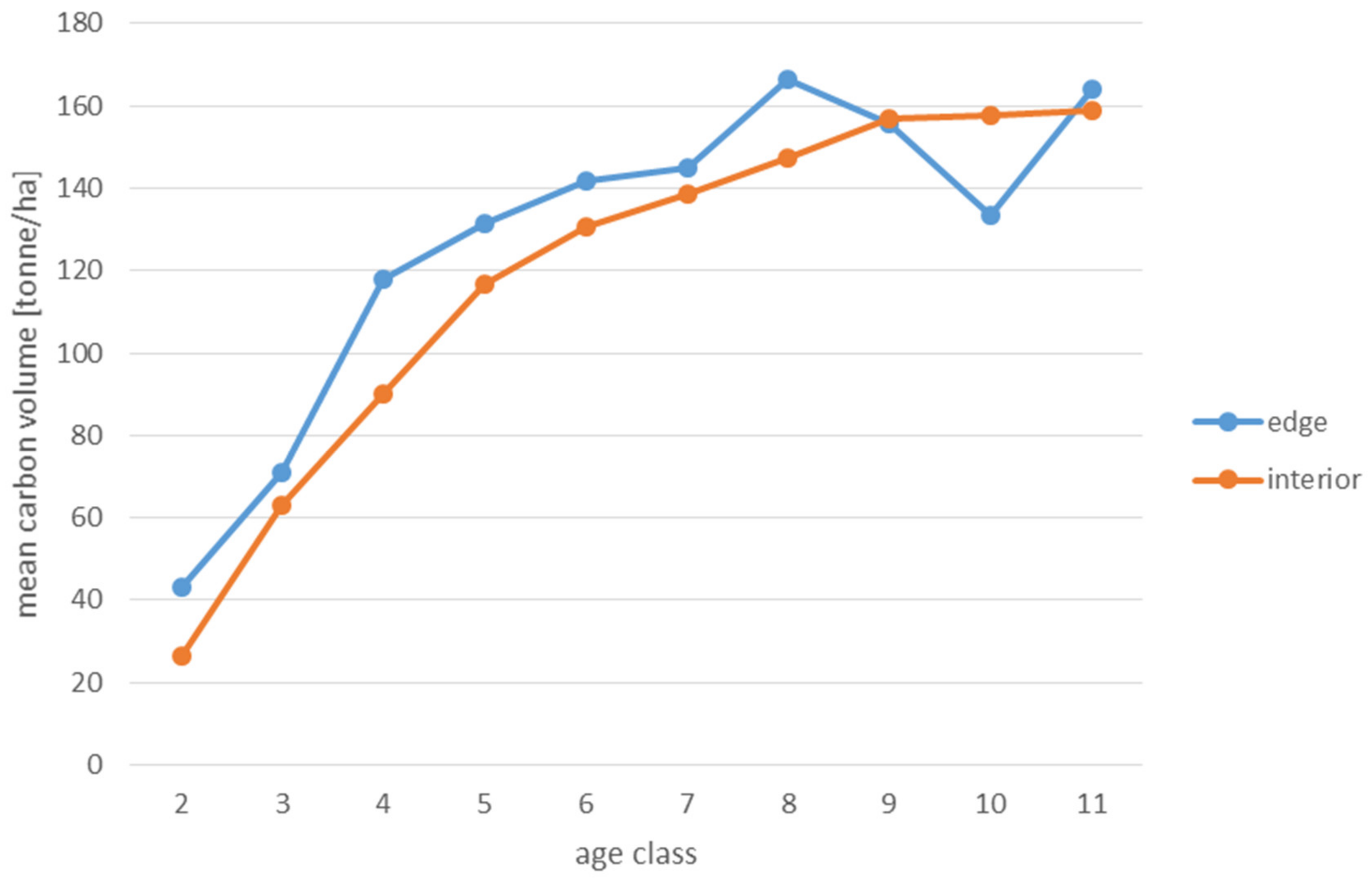
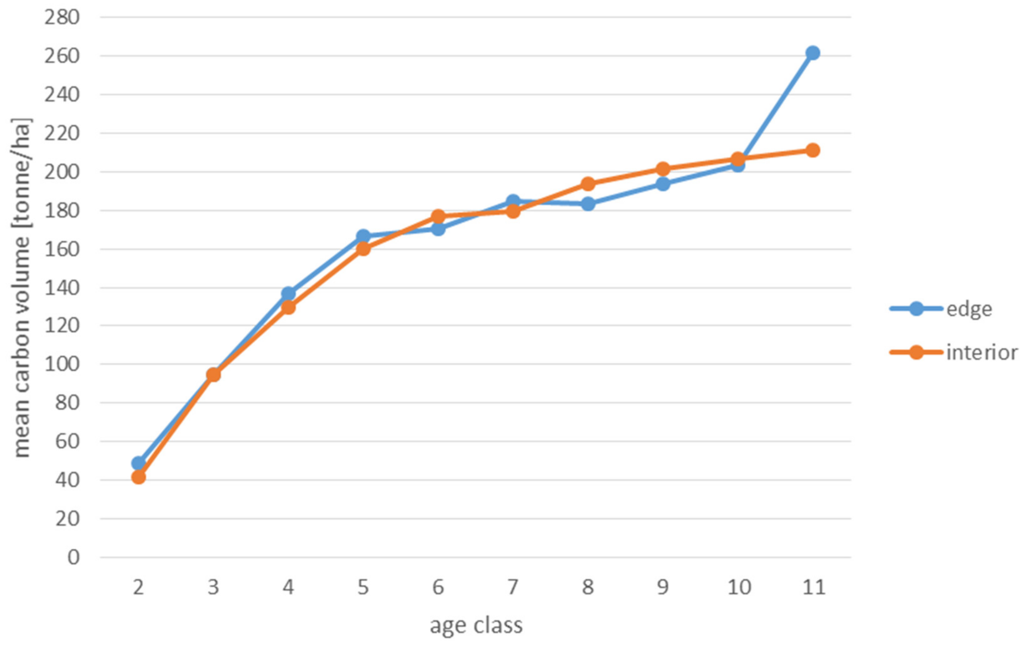
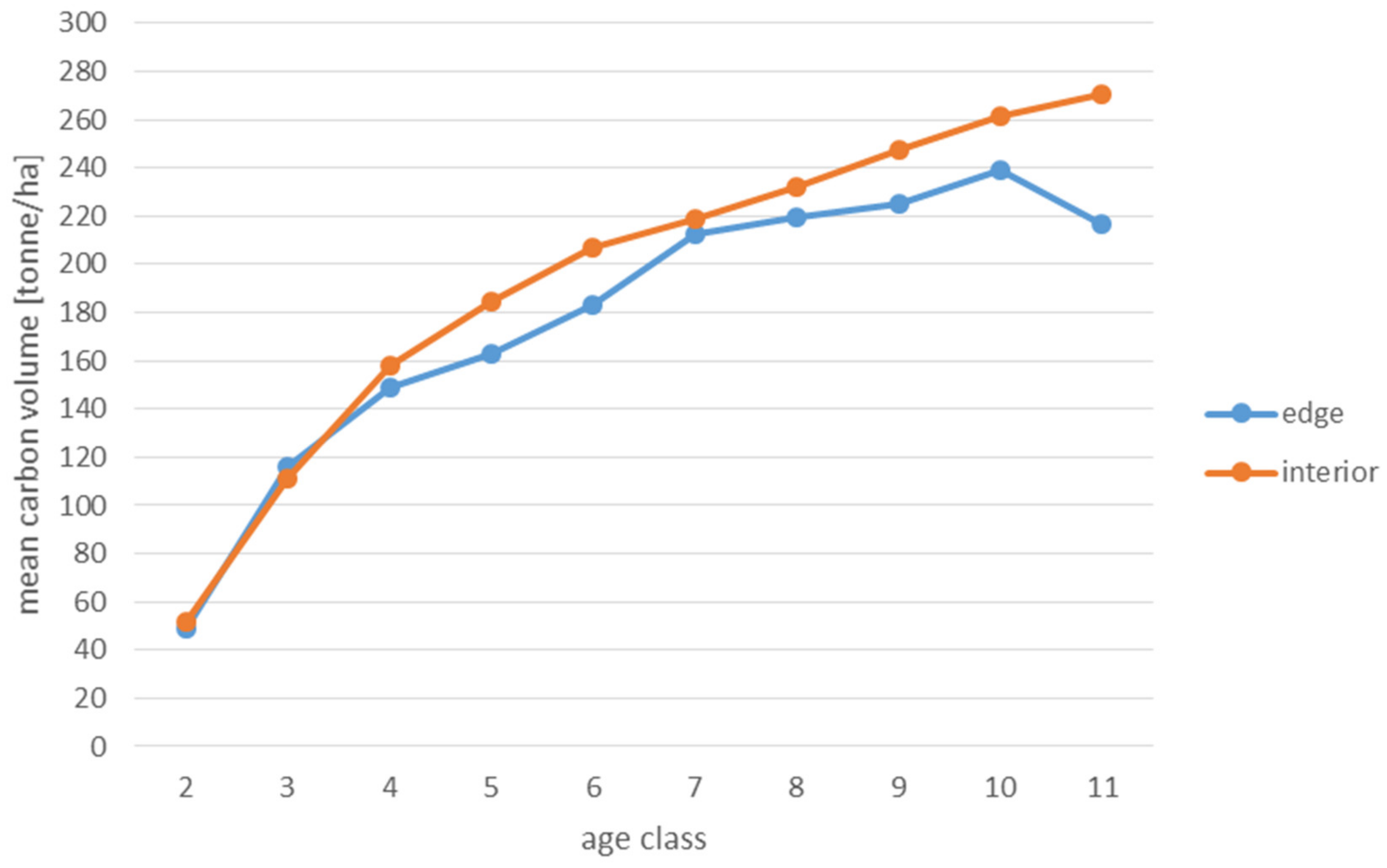
Analyses of the volume of carbon accumulated in the living biomass in the edge zone and in the interior zone were also used to assess the effects of forest fragmentation. For this purpose, the volume of the growing stock (m
3) had to be converted to tonnes of carbon (C). The method proposed by the Intergovernmental Panel on Climate Change was used [
68]. Appropriate coefficients were used to evaluate the amount of carbon accumulated in the living biomass according to the actual species composition of the stands on the plots. The calculation was made using the Equation (2):
where:
C–carbon in tonnes,
V–growing stock volume (m3),
BCEF–biomass conversion and expansion factor,
R–root factor,
CF–carbon fraction [tonne C (tonne dry matter)-1].
The values of
BCEF,
R, and
CF coefficients as a function of tree species and tree age were taken from tables published by the IPCC [
68]. When a tree species was not included in the IPCC tables, the values for pine were used in the case of coniferous species and for hornbeam in the case of deciduous species. The amount of carbon used to present the results is expressed in the unit t/ha (tonnes per hectare).
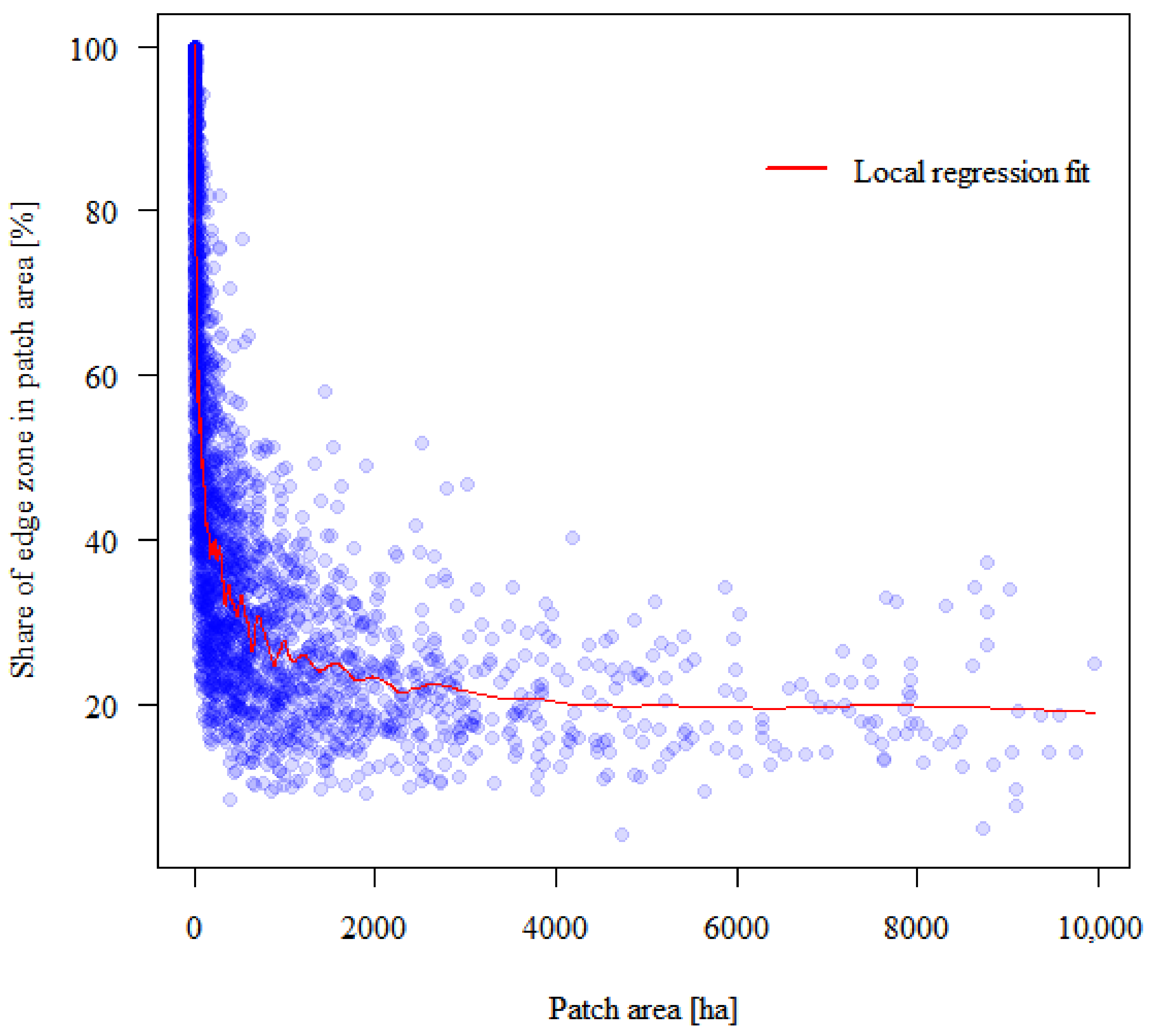
In the last stage of calculations, based on spatial analysis, the critical area of the forest patch was determined, above which the average share of the edge zones was considered a constant value. In other words, it is the size of the forest patch above which the impact of the edge effect on the volume of wood resources is considered insignificant. To this end, the local regression model was adjusted to determine the approximate area where the curve flattens. The determination of the curve near each point referred to 5% of the closest patches in terms of area, which should make the regression very local.


