Article

Comparison of Machine Learning Methods Applied on Multi-Source Medium-Resolution Satellite Images for Chinese Pine (Pinus tabulaeformis) Extraction on Google Earth Engine

1
College of Forestry, Inner Mongolia Agricultural University, Hohhot 010019, China
2
Key Laboratory of Forestry Remote Sensing and Information System, NFGA, Chinese Academy of Forestry, Beijing 100091, China
3
School of Geomatics, Liaoning Technical University, Fuxin 123000, China
4
The Institute of Chifeng Forestry Research, Chifeng 024000, China
*
Author to whom correspondence should be addressed.
Forests 2022, 13(5), 677; https://doi.org/10.3390/f13050677
Submission received: 25 March 2022 / Revised: 21 April 2022 / Accepted: 26 April 2022 / Published: 28 April 2022
(This article belongs to the Section Forest Inventory, Modeling and Remote Sensing)

Abstract

:
Chinese pine has tremendous applications in many fields. Mapping the distribution of Chinese pine is of great importance for government decision-making and forest management. In order to extract Chinese pine on a large scale, efficient algorithms and open remote-sensing datasets are needed. It is widely believed that machine learning algorithms and medium-resolution remote-sensing datasets can work well for this purpose. Unfortunately, their performance for Chinese pine extraction has remained unclear until now. Therefore, this study aims to explore the ability of the different machine learning algorithms and open remote-sensing datasets for Chinese pine extraction over large areas on Google Earth Engine (GEE). So, based on the combination of three typical machine learning algorithms, namely deep neural network (DNN), support vector machine (SVM), random forest (RF), and three open medium-resolution remote-sensing datasets, namely Sentinel-2, Gaofen-1, and Landsat-8 OLI, 27 models are constructed and GEE, with its powerful computing ability, is used. The main findings are as follows: (1) DNN has the highest accuracy for Chinese pine extraction, followed by SVM and RF; DNN is more sensitive to spatial geometric information, while SVM and RF algorithms are more sensitive to spectral information. (2) Spectral indexes are helpful for improving the extraction accuracy of Chinese pine. The extraction accuracy by using Gaofen-1 dataset increases 7.6% after adding spectral indexes, while the accuracies by using Sentinel-2 and Landsat-8 datasets increase 1.8% and 1.9% after adding spectral indexes, respectively. (3) The extraction accuracy by using DNN and Sentinel-2 dataset with spectral indexes is the highest, with an overall accuracy of 94.4%. (4) The area of Chinese pine is 153.73 km2, accounting for 5.06% of the administrative area of Karaqin Banner, and it is convenient to extract Chinese pine on a large scale by using GEE.

1. Introduction

Forest ecosystems play an irreplaceable role in conserving and improving ecosystem functions [1,2]. As one of the tree species native to northern China, Chinese pine is not only resistant to hot and dry environments but also can withstand winter frost because of its strong stress resistance [3,4,5]. Therefore, Chinese pine has become the main afforestation tree species in northern China and is of great significance for improving the ecological environment [6,7,8,9]. Chinese pine also has a wide range of medicinal and industrial uses [8,9,10]. Due to its irreplaceable value, the Chinese government started to plant Chinese pine artificially in the 1980s and a vast area of near-mature and mature forests have now formed. Thus, accurate extraction and monitoring of Chinese pine is of great value for ecological environment protection, sustainable forest management, and industrial production. However, it is mainly distributed on the steep slopes of mountainous areas and is scattered [11]. The traditional human investigation method is not only laborious but also dangerous and inaccessible. The development of remote-sensing technology makes it possible to detect Chinese pine in a large area and with high timeliness.
In recent years, machine learning algorithms have been widely used in the field of ground object classification and extraction [12,13,14,15,16,17]. In order to find an algorithm with better accuracy, scholars have compared the performance of numerous machine learning algorithms [18,19,20]. The results show that it is difficult to find a specific machine learning algorithm that is suitable for all pattern-recognition tasks. Different algorithms often lead to different results because of the differences in texture and spectrum of the ground objects. For example, Raczko et al. [21] compared three machine learning methods for tree-species classification applied on airborne hyperspectral images, namely SVM, RF, and artificial neural networks (ANN). The results show that ANN outperforms SVM and RF. Qian et al. [22] classified the land cover types using four methods including k-nearest neighbor (KNN), normal bayes (NB), classification and regression tree (CART), and SVM, and found that SVM and NB exhibited the best performance. Forkuor et al. [23] used multiple linear region, random forest regression, SVM, and stochastic gradient boosting (SGB) to map the spatial distribution of six soil properties. It was found that random forest regression achieves the highest accuracy in most cases. Ge et al. [24] compared KNN, RF, SVM, and ANN for land-use/-cover classification in an arid desert-oasis mosaic landscape of China; the highest overall accuracy was produced by the ANN (97.16%), closely followed by the RF (96.92%), SVM (96.20%) and KNN (93.98%). Zhou et al. [25] used CART, RF, and SVM to detect dump sites for construction and destruction waste. In order to obtain the optimal extraction results, the internal parameters of the algorithm are optimized. The results show that RF performs best, followed by SVM and CART. Which machine learning algorithm is much more suitable for Chinese pine extraction has remained unclear until now.
Various remote-sensing data have been used to obtain forest parameters, including light detection and ranging (LiDAR) [26], high-resolution remote-sensing images [27], hyperspectral remote-sensing images [28], synthetic aperture radar (SAR) [29], and the combination of them [30]. However, most of these remote-sensing data are expensive and cannot be obtained easily, meaning that studies using these data can only be carried out in small areas. In contrast, the open medium-resolution remote-sensing datasets are highly suitable for studies of large areas because of their wide coverage and high temporal resolution and because they are free of charge [26]. Sentinel-2, Gaofen-1 WFV and Landsat-8 OLI are three frequently used open medium-resolution remote-sensing datasets, which can be downloaded from the internet worldwide. They have been used in areas such as tree-species classification and extraction, estimation of the leaf area index (LAI), mapping forest aboveground biomass, forest cover change analysis, forest fire detection, forest canopy closure estimation, etc. [31,32,33,34]. Spectral indexes are helpful for distinguishing different objects. Due to the differences in spatial and spectral resolution of Sentinel-2, Gaofen-1 WFV, and Landsat-8 OLI, researchers have already carried out some work to explore their performance for object classification and extraction in many fields [35,36,37,38].
Previously, remote-sensing images had to be downloaded from the internet and preprocessed manually by using software such as ENVI, Erdas, PCI, etc., which was time and labor consuming. The classification and extraction tasks in large areas consume a lot of computing resources and computer memory. Google Earth Engine (GEE) is a cloud computing platform developed by Google [39]. It has powerful computing ability and can process remote-sensing datasets easily. Because of this, it is widely used in transportation, surveying and mapping, agriculture, forestry, and other fields [40,41,42,43,44,45].
Chinese pine is an evergreen tree species. Its spectral reflectance changes slightly with age. In order to accurately extract Chinese pine on a large scale, efficient algorithms and open remote-sensing datasets are needed. As mentioned above, it can be argued that machine learning algorithms and medium-resolution remote-sensing datasets can work well for this purpose. Unfortunately, their performance for Chinese pine extraction has remained unclear until now; therefore, this study aims to explore the ability of the different machine learning algorithms and open remote-sensing datasets for Chinese pine extraction over large areas on GEE: The goals of this study include five aspects: (1) to explore the ability of DNN, SVM, and RF for Chinese pine extraction distributed across a large area; (2) to explore the influence of different datasets on the extraction accuracy of Chinese pine by using the three algorithms; (3) to make full use of the bands provided by Sentinel-2 Level-2A, GF1 and Landsat-8 OLI and explore their potential for the extraction of Chinese pine; (4) to explore the influence of the spectral indexes (NDVI, NDWI, EVI and MSAVI) on the accuracy of Chinese pine extraction; and (5) to analyze the feasibility of different data sources and different methods for the extraction of Chinese pine in different application scenarios by comparing the accuracy.

2. Materials and Methods
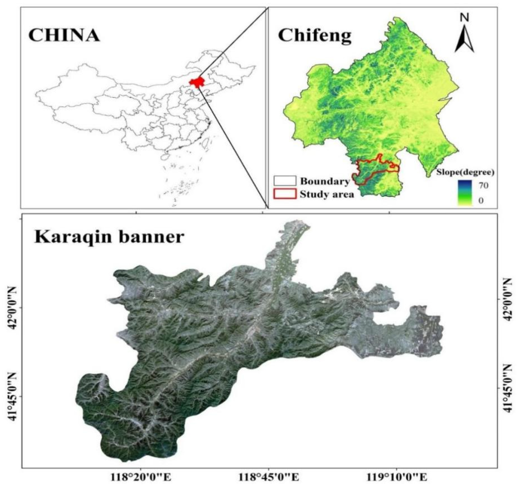
2.1. Study Area

Karaqin Banner is selected as the study area, which lies to the eastern part of the Inner Mongolia in northeastern China (Figure 1). The total land area is 3050 square kilometers with a complex topography dominated by mountains and hills. The altitude is 856–1460 m and the slope is between 15 and 35 degrees. The soil is mainly cinnamon and brown soil, and the soil types are mostly semi-arid and stony. It belongs to the semi-arid continental monsoon climate of the middle temperate zone, and the climate changes greatly across the four seasons. The winter is cold with little snow, the spring is dry and windy, the summer is short and hot, and the temperature drops rapidly in autumn. The average annual precipitation is about 400 mm, mostly concentrated from July to September, and the annual evaporation is 2280 mm. According to the local conditions, the trees are mainly Chinese pine, the shrubs are Caraganakorshinskii and Vitexnegundo Far. Heterophylla, and the main grasses are Astragalus adsurgens and Melilotus officinalis [46,47].

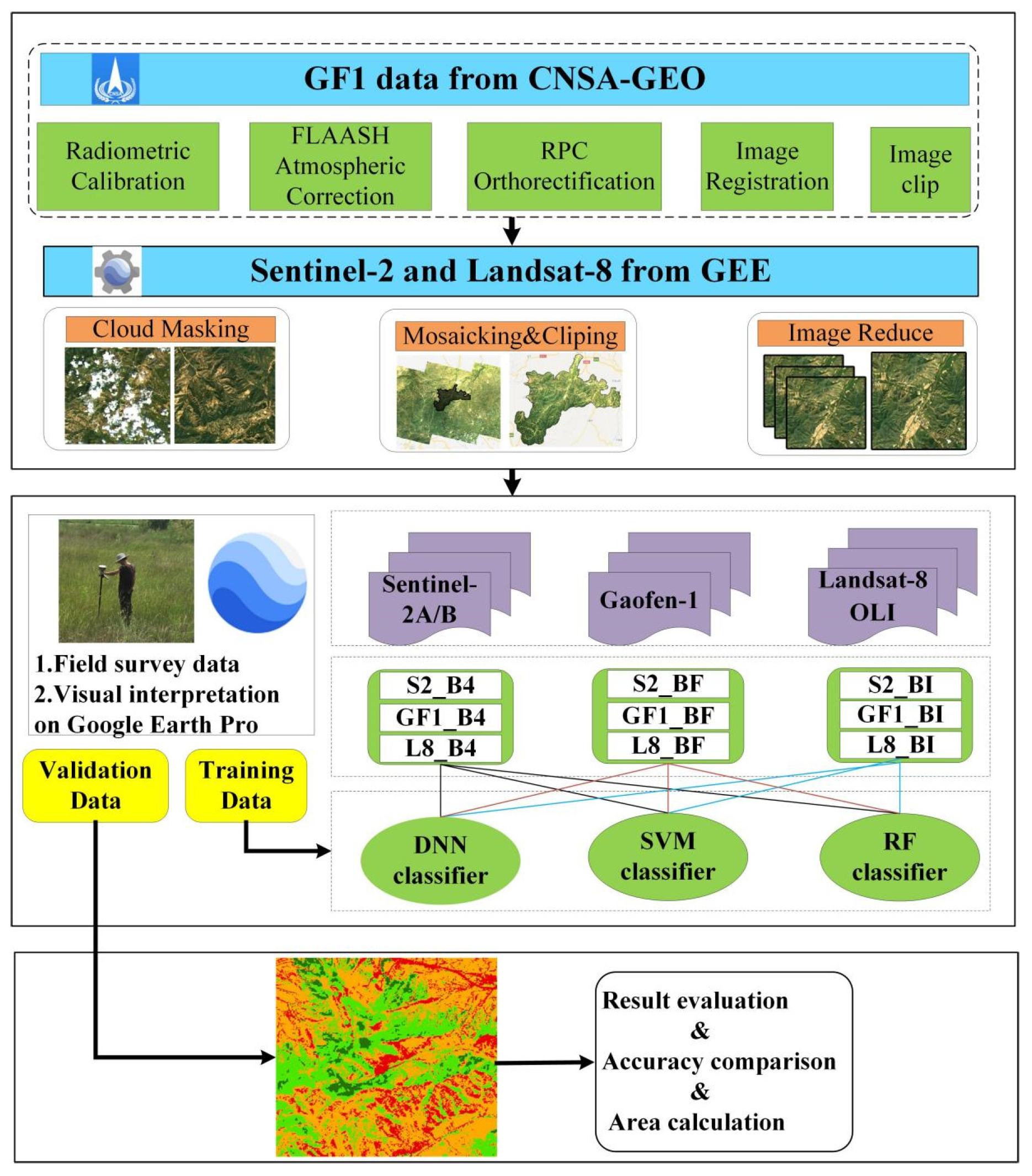
2.2. Data Acquisition and Preprocessing

2.2.1. Remote-Sensing Data

In this study, three types of medium-spatial-resolution satellite remote-sensing images were used, including Sentinel-2 (10 m), Gaofen-1 WFV (16 m), and Landsat-8 OLI (30 m). The Level-2A product of Sentinel-2 data was used, which can be found in the COPERNICUS/S2_SR dataset on GEE, as well as the L1TP level product of Landsat 8 OLI data from the LANDSAT/LC08/C01/T2_SR dataset. Both of them are atmospherically corrected surface reflectance and have been preprocessed, namely by resampling, reprojection, and image reduction using images dated from 1 September 2017 to 30 September 2017, cloud mask (<10%), and clipping. Gaofen-1 is a Chinese remote-sensing satellite. From November 2019, Gaofen-1 WFV data with four bands (blue, green, red, near-infrared) and a width of 200 km began to be shared globally, and users can register and download data through the platform of CNSA-GEO (Available online: http://www.cnsageo.com/ (accessed on 15 November 2021). The data from 2013 to 2019 can be downloaded. The Gaofen images used in this article had already had preprocessing carried out before using, e.g., radiometric calibration, atmospheric correction, ortho-rectification, and geometric correction; the radiometric calibration parameters can be obtained from the website of China Centre for Resources Satellite Data and Application (Available online: http://www.cresda.com/CN/index.shtml (accessed on 18 November 2021).

2.2.2. Datasets Used in the Study

Three datasets are established by using Landsat-8 OLI(L8), Gaofen-1 WFV(GF1) and Sentinel-2 (S2) remote-sensing images, namely, the four-bands (B4) dataset, full-band (BF) dataset, and spectral indexes (BI) dataset. The B4 dataset is a combination of red, green, blue, and near-infrared of different remote-sensing data, including the B4 dataset of Sentinel-2 (S2_B4), B4 dataset of Gaofen-1 (GF1_B4), B4 dataset of Landsat 8 OLI (L8_B4). In order to explore the full-band extraction ability of Chinese pine, all bands shown in Table 1 were used, and the full-bands dataset of Sentinel-2(S2_BF) was established, as well as the full-bands dataset of Gaofen-1(GF1_BF) and the full-bands dataset of Landsat-8 OLI(L8_BF). It can be seen from Table 1 that S2_BF consists of 13 bands, GF1_BF consists of 4 bands, and L8_bands consists of 13 bands. Spectral indexes, including the normalized difference vegetation index (NDVI) [48], normalized difference water index (NDWI) [49], enhanced vegetation index (EVI) [50], and modified soil-adjusted vegetation index (MSAVI) [51], were calculated before building spectral index datasets. The formulas are shown in Table 2. The Sentinel-2 spectral index dataset (S2_BI), Gaofen-1 WFV spectral index dataset (GF1_BI), and Landsat 8 OLI spectral index dataset (L8_BI) were established based on adding the four spectral indexes to the datasets of S2_BF, GF1_BF, and L8_BF, respectively.

2.2.3. Training Data

The field survey was conducted from 1–25 August 2017 in Karaqin Banner, Chifeng. The land-use types are divided into construction land, cultivated land, other woodlands, Chinese pine, and other land types. In order to improve the efficiency, the survey area was divided into 7 sub-areas in the east–west direction and carried out along the roads. The global positioning system (GPS) with an accuracy of ±5 m was used to record the geographic location of the sampling point, and the corresponding feature types were recorded in the paper at the same time. Through visual interpretation and prior knowledge, sample points were collected by using Google Earth Pro; a total of 979 sample points were obtained, of which 754 were training samples and 225 were test samples. The point information and landcover types are shown in Table 3. All the sample points (training and testing) were merged into one layer and added with a unique identification field, namely 0 (construction land), 1 (cultivated land), 2 (other woodland), 3 (Chinese pine), and 4 (other land types). Finally, they were uploaded to GEE in the format of shapefiles.

3. Method

Firstly, the preprocessed Gaofen-1 WFV remote-sensing images were uploaded to the Google Earth Engine platform. Combining with Landsat-8 OLI and Sentinel-2 data from GEE, three datasets were established. Through field survey and visual interpretation, a point samples dataset was generated according to the spectral features, texture features, geometric morphological features, location information, etc. Three machine learning algorithms, including two shallow learning methods (RF and SVM) and one deep-learning method (DNN), were used to extract Chinese pine. In order to implement the three algorithms, GEE, Colab, and Google cloud platform (GCP) were used. Finally, the extraction results of Chinese pine were evaluated and the area of Chinese pine in Karaqin Banner was calculated. The workflow chart is shown in Figure 2.

3.1. RF

RF is an ensemble learning method in machine learning. The classifier was first proposed by Leo Breiman [52]. It is composed of many weak classifier decision trees. By using bootstrap aggregating (bagging), m samples are randomly selected from the M samples (m < M), and n samples are randomly selected from all the N features (n < N) to build decision trees that can make predictions on the data. Since the decision trees trained by different data are different from each other, the final results are finally decided by voting. Due to the randomness of the sample and feature selection, RF has the advantages of strong noise resistance, generalization ability, and a strong processing ability for high-dimensional data, without needing to select features manually. On the platform of GEE, the smile Random Forest function (smile Random Forest) is used, and the number of decision trees is set to 50 [25].

3.2. SVM

SVMs are supervised learning models that analyze data used for classification and regression analysis, first proposed by Vapnik and Chervonenkis in the framework of the “Generalised Portrait Method” for computer learning and pattern recognition. The development of these ideas started in 1962 and they were first published in 1964, with advantages in solving the problems such as being nonlinear and high dimensional in the field of pattern recognition [53]. A decision boundary is used to separate the positive and negative examples with a straight line or plane, and the distance between the decision boundary and two margin boundaries passing through the support vector should be as far as possible. However, it is usually difficult to find a straight line or a hyperplane to separate the data linearly from each other. In order to solve this problem, Cortes and Vapnik proposed a soft margin SVM in 1995 [54], which introduces a fault-tolerance rate to allow a small number of samples to be misclassified when most samples are separated properly; kernels are used to map the training data from the low-dimensional space to the high-dimensional space, aimed at constructing a decision surface between different classes. The commonly used kernels include linear, nonlinear, polynomial, Gaussian kernel, radial basis function (RBF), sigmoid, etc. RBF has the advantages of fewer parameters and a better performance. In this study, the function of libSVM in GEE is used and the kernel function of RBF is chosen, with gamma = 16 and cost = 34 [25].

3.3. DNN

DNN, also known as the multi-layer perceptual neural network, consists of an input layer, hidden layer, and output layer. It has a deep structure and can describe complex problems [55]. Hidden layers are one of the most important parts of neural networks. In the network of this study, there are 5 hidden layers. In order to prevent the disappearance of the gradient, the ReLU activation function is used, and softmax is used as the loss function. The DNN is implemented on the Keras framework based on TensorFlow. The initial learning rate is 1 × 10⁻⁵. The network weights are updated a total of 2000 times. In the process, Colab is used to write the code, and the model generated after training is stored in the Google Cloud platform. Finally, the model is called through GEE to predict the remote-sensing images of the study area.

3.4. Accuracy Assessment

The confusion matrix, also known as the error matrix, is a standard matrix for expressing accuracy evaluation. It is mainly used to compare classification results and actual classes. The overall accuracy (OA), consumer accuracy (CA), producer accuracy (PA), and kappa coefficient are the four indicators that are often used for evaluation. In order to evaluate the Chinese pine extraction results, 183 verification sample points are obtained through field investigation and a confusion matrix was made. The OA and kappa coefficient are selected to evaluate the results quantitatively, expressed as Equations (1) and (2). Additionally, in order to evaluate the result qualitatively, visual interpretation is also operated in this study by using the tools Google Earth Pro and QGIS.
OA = i = 1 n x i i / N
kappa = N i = 1 n x i i i = 1 n ( x i + x i + 1 ) N 2 i = 1 n ( x i + x i + 1 )

4. Results and Analysis

Chinese pine is distributed scattered and unevenly. In order to illustrate the extraction results of different models, three regions with different shapes in the Karaqin Banner are selected for display. Each of them includes Chinese pine, construction land, other woodlands, and cultivated land. It can be seen from the figures that Chinese pine is significantly different from other classes in texture and spectrum. Figure 3 shows one of the 27 extraction results of Chinese pine extraction results in the Karaqin Banner.

4.1. Comparison of Extraction Results of Different Machine Learning Methods on B4 Datasets

The size of the objects and the spatial resolution of the remote-sensing images can both affect the classification accuracy by the means of remote sensing. Studies have shown that it is not the case that the higher the spatial resolution, the higher the classification accuracy; the key is to choose the spatial resolution that is suitable for the scale of the ground objects [56,57]. Therefore, the ability of remote-sensing images with different spatial resolutions should be explored so as to better obtain the distribution and change information of Chinese pine. The four-bands datasets, including S2_B4, GF1_B4, and L8_B4 with the same spectral resolution (red, green, blue, near-infrared) and different spatial resolution ranges from 10 to 30 m, were used for Chinese pine extraction combined with the machine learning methods (DNN, SVM and RF).
As can be seen from Figure 4 and Figure 5, generally speaking, each algorithm can identify Chinese pine. However, there are differences in the details. For example, DNN can separate Chinese pine from other forests well, SVM and RF cannot completely identify Chinese pine, and they incorrectly classify other forests as Chinese pine. The cultivated land and construction land are not misclassified as Chinese pine. The difference between SVM and RF is not obvious. With the spatial resolution decrease from 10 to 30 m, the extraction accuracy of Chinese pine along the boundary of the shown area (Figure 4) became inferior, and the sawtooth phenomenon occurred. The L8_B4 dataset had the most obvious sawtooth phenomenon as its lowest spatial resolution.
Figure 6a,b show the OA and kappa coefficient of pine extract. It can be seen that the OA and kappa coefficient have the same trend of change. The OA levels of the three algorithms rank as: RF < SVM < DNN, and the OA levels of three datasets rank as: L8_B4 < GF1_B4 < S2_B4. Among the nine models, DNN_S2_B4 has the highest accuracy, whose OA is 88.5% and kappa coefficient is 0.866; RF_L8_B4 has the lowest accuracy, whose OA is 76.6% and kappa coefficient is 0.687. The difference in OA and kappa coefficient between DNN_S2_B4 and RF_L8_B4 is 11.9% and 0.179, respectively. The differences in the accuracies of SVM_S2_B4 and DNN_GF1_B4 are the smallest, only 0.3% for OA and 0.034 for the kappa coefficient. The difference in OA between SVM_GF1_B4 and RF_S2_B4 is 40%, and the difference between DNN_S2_B4 and SVM_S2_B4 is 0.44.

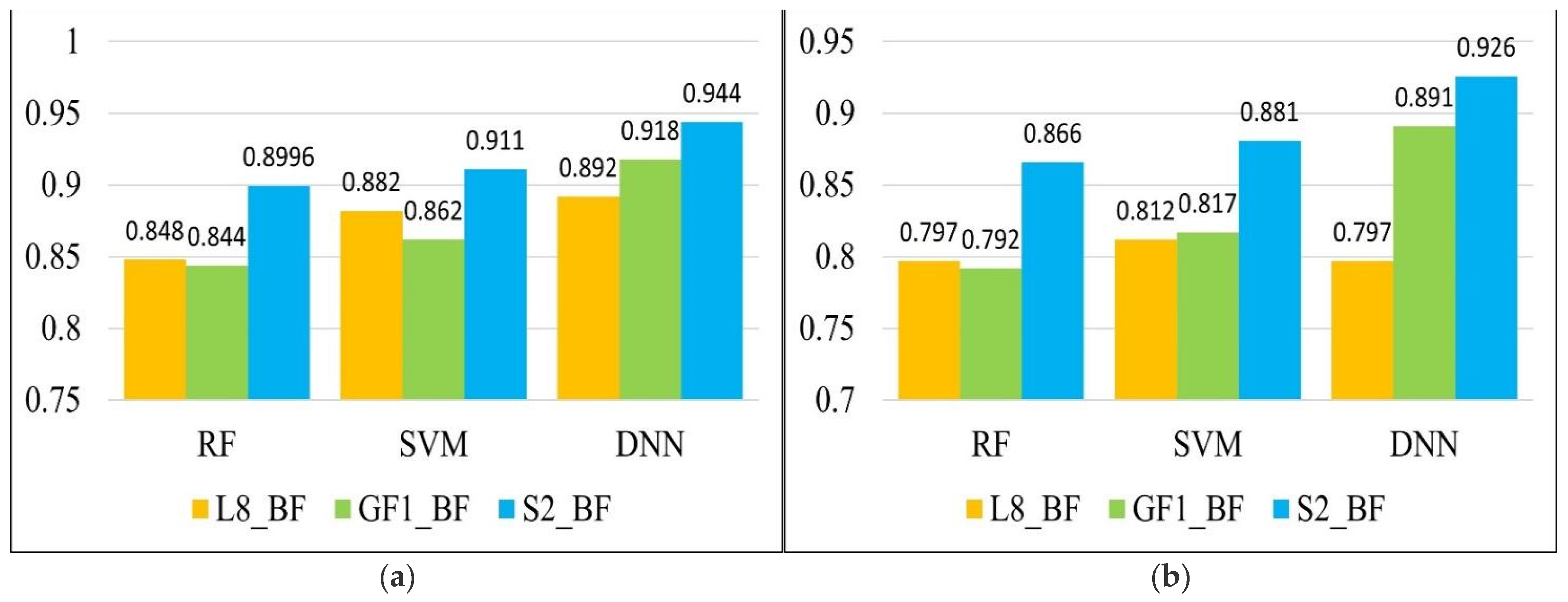
4.2. Comparison of Extraction Results of Different Machine Learning Methods on BF Datasets

Different remote-sensing images have different spectral characteristics. Sentinel-2 Level-2A, Gaofen-1, and Landsat-8 OLI contain 13 bands, 4 bands, and 9 bands, respectively, which can be used for ground-object classification. The specific band information is shown in Table 2. In the field of tree-species identification and classification, Sentinel-2, Gaofen-1, and Landsat-8 OLI data have been widely used [58,59,60]. However, only a part of each band was selected. In order to make full use of the spectral information provided by remote-sensing images, and to explore their potential for the extraction of Chinese pine, all the bands of Sentinel-2 Level-2A, Gaofen-1, and Landsat-8 OLI should be used.
As shown in Figure 7 and Figure 8, the extraction result of Chinese pine on the S2_BF dataset is the best, followed by L8_BF. The number of Chinese pine pixels misclassified as other woodlands in GF1_BF is higher than S2_BF and L8_BF (Figure 8b). This is because the spectral resolution of GF1_BF is lower than the other two datasets, although its spatial resolution is higher than L8_BF. In addition, due to the low spatial resolution of L8_BF, the Chinese pine in the boundary area is not correctly identified (Figure 8c); S2_BF has a much better performance because of the higher spatial resolution and spectral resolution, and it can better distinguish Chinese pine and other tree species (Figure 8a).
It can be seen from Figure 9a that the OA of all models was above 0.8, and they achieved good results. The OA of DNN_S2_BF is as high as 91.8%, and the OA of RF_GF1_BF is 83.3%, which is the lowest of the BF models. As can be seen from Figure 9a,b, the OA and kappa levels of the datasets rank as: RF_GF1_BF < RF_L8_BF, SVM_GF1_BF < SVM_L8_BF, indicating that spectral information plays a much more important role than spatial information in extracting Chinese pine using RF and SVM. However, the accuracy of DNN_GF1_BF is higher than DNN_L8_BF, showing that DNN is more sensitive for spatial geometric information than spectral information.

4.3. Comparison of Extraction Results of Different Machine Learning Methods on BI Datasets

In order to explore the influence of spectral indexes on the Chinese pine extraction, four typical spectral indexes (NDVI, NDWI, EVI, and MSAVI) were added to the datasets of BF (S2_BF, GF1_BF, and L8_BF), and three spectral indexes datasets (S2_BI, GF1_BI, and L8_BI) were constructed. Spectral indexes are widely used in tree-species classification and identification [61,62,63,64]. However, to our knowledge, there is no report on the evaluation of applying the spectral index on the Chinese pine extraction.
In the nine model-classification results with the addition of spectral indexes, the misclassification of Chinese pine and other classes is significantly reduced (Figure 10 and Figure 11). There is no obvious difference between the nine Chinese pine extraction results below. As shown in Figure 12a, the OA of the nine models were all above 84%, of which the OA of DNN_S2_BI reaches as high as 0.944, and the OA of RF_GF1_BI is the lowest, but also reached 84.4%. The band numbers of S2_BI, GF1_BI, and L8_BI are 17, 8 and 13, respectively. Although the spatial resolution of GF1_BI (16 m) is higher than that of L8_BI (30 m), the accuracies of SVM_GF1_BI (0.862) and RF_GF1_BI (0.844) are slightly lower than those of SVM_L8_BI (0.882) and RF_L8_BI (0.848). The higher spectral resolution of the SVM_L8_BI and RF_L8_BI make up for their lack of spatial resolution for Chinese pine extraction. The OA of DNN_GF1_BI is 91.8%, and the OA of DNN_L8_SI is 0.89.2%, indicating that DNN is more sensitive to spatial information than spectral information. The results of Chinese pine extraction are better when using BI datasets compared with B4 and BF. The kappa coefficient has the same trend as OA (Figure 12b).

4.4. Comprehensive Analysis and Area Estimation

As shown in Figure 13, the extraction accuracy of Chinese pine is improved with the increase in spatial and spectral resolution of remote-sensing images. For Sentinel-2, the average OA increased by 3.3% from S2_B4 (13 bands) to S2_BI (17 bands) by using the three algorithms (DNN, SVM, and RF), and 1.8% from S2_BF (13 bands) to S2_BI (17 bands). For Gaofen-1, the average OA increased 7.6%t from GF1_B4 (4 bands) to GF_BI (8 bands); for Landsat-8 OLI, the average OA increased 8.8% from L8_B4 (4 bands) to L8_BF (9 bands), and 1.9% from L8_BF (9 bands) to L8_BI (13 bands). The above analysis shows that increasing the spectral resolution and adding spectral indexes can improve the extraction accuracy of Chinese pine. It is worth mentioning that the Gaofen-1 extraction accuracy increased by 7.6% after adding spectral indexes, which is higher than Sentinel-2 (1.8%) and Landsat-8 OLI (1.9%).
For S2 (Sentinel-2) datasets, the OA can reach as high as 94.4% by DNN, 91.1% by SVM, and 90% by RF. For GF1 (Gaofen-1) datasets, the highest accuracy is 0.918 by DNN, 0.862 by SVM, and 0.844 by RF. For Landsat-8 OLI (L8) datasets, the highest accuracy was 0.892 by DNN, 0.882 by SVM, and 0.848 by RF. Based on the above analysis, among the three machine learning algorithms (DNN, SVM, and RF), DNN has the highest extraction accuracy for Chinese pine, followed by SVM and RF. Since the highest OA of these three algorithms can all reach above 0.8, SVM can be selected for Chinese pine extraction in the cases with limited computing resources.
All of these 27 models are used to calculate the total area of Karaqin Banner and the Chinese pine area in Karaqin Banner. As shown in Table 4, the total area calculated on Sentnel-2, Gaofen-1, and Landsat-8 OLI is 3037.41 km2, 3036.30 km2, and 3036.75 km2, respectively, which has about a 13 km2 difference from the officially announced 3050 km2. As shown in Figure 14, the extraction result of Chinese pine on the DNN_S2_BI dataset is 153.73 km2, accounting for 5.06% of the total area of Karaqin Banner.

5. Discussion

In recent years, much more attention has been paid to the environmental problems by the international communities [65,66,67]. As one of the main afforestation tree species in northern China, Chinese pine has strong stress resistance, which can withstand drought and cold and grow well in acidic, neutral, and barren soil. It is of great significance for absorbing carbon dioxide, improving the environment, and for soil and water conservation. Chinese pine also has a wide range of industrial and medicinal uses [5,6,7,8,9,10].
Chinese pine is widely distributed and scattered. It is not only time and labor consuming to investigate Chinese pine by manpower, but also dangerous. With the development of data-acquisition technology, more and more remote-sensing datasets are used in forest resource surveys, but most remote-sensing data can only be applied to small areas due to high cost. In terms of the algorithms, although machine learning has been widely used in many fields, its performance in Chinese pine extraction is still unknown. Google Earth Engine (GEE) is a cloud computing platform that can easily acquire large-scale remote-sensing data and quickly complete preprocessing. The main goals of this research are to explore the performance of machine learning algorithms and publicly available medium-resolution remote-sensing datasets in large-area extraction of Chinese pine on GEE, and to provide references for further Chinese pine extraction in larger areas.
It is known from the experiment that the extraction accuracy of Chinese pine is related to machine learning algorithms and the spatial and spectral resolution of the remote-sensing datasets used. In terms of algorithms, DNN has the highest extraction accuracy, followed by SVM, and RF is the lowest. In some classification and extraction tasks, it is believed that it is not the case that the higher the spatial and spectral resolution, the better the extraction accuracy [56,57]. In this experiment, the extraction accuracy of Chinese pine increases with the improvement of the spatial and spectral resolution of remote-sensing datasets. The use of spectral indexes (NDVI, NDWI, EVI and MSAVI) plays a positive role in improving the extraction accuracy. Although Karaqin Banner has arid climatic conditions with little precipitation, Chinese pine, with its strong adaptability, accounts for 5.06% of the total area of the administrative area, which is a very high proportion. There is much more Chinese pine in the west part of Karaqin Banner than in the east; the main reason is that the terrain in the west is dominated by mountains and hills, which is very suitable for the growth of Chinese pine, but the eastern part is relatively flat.
Although the DNN_S2_BI model has the highest accuracy, the Sentinel-2 satellites can only provide remote-sensing images from 2015 to the present, which are insufficient for long-term sequence analysis. However, Landsat satellites have continuously acquired space-based images of the Earth’s land surface since 1972 [68]. It can be found through the experiments that the OA can be close to 90% by selecting appropriate methods and datasets of Landsat. Therefore, Landsat is a better choice for long time series analysis of Chinese pine. Gaofen-1 has a temporal resolution of 4 days, which is shorter than Sentinel-2 (5 days) and Landsat (16 days), but with a lower spectral resolution of 4 bands. Its spatial resolution is 16 m, between Sentinel-2 and Landsat. By adding the spectral indexes, the extraction accuracy can be as high as 91.8%. However, it is difficult to extract Chinese pine precisely with the influence of clouds and fog in the optical remote-sensing images. The comprehensive application of these three remote-sensing satellites can effectively remove the influence of weather. As one of the algorithms in the field of deep learning, DNN has the highest extraction accuracy for Chinese pine compared to SVM and RF, but it requires more computing power and storage space, and the training time is longer than that of SVM and RF.
However, the research still has some limitations, which should be explored in the future. For example, during the extraction of Chinese Pine, only medium-resolution remote-sensing images are used; the ability of high-spatial-resolution (<10 m) remote-sensing images for Chinese pine extraction should be explored in future. On the other hand, the point samples with the advantage of being easier to obtain are used for training in this study, although it can also achieve reliable precision in the extraction of Chinese pine. Semantic features of remote-sensing images are not fully utilized, resulting in speckle noise and extraction errors. In recent years, convolution neural networks have been widely used in the field of remote-sensing image recognition and have achieved good results [69,70,71,72]. Therefore, it is necessary to study the potential of applying convolutional neural networks for Chinese pine extraction in the future. Finally, the research failed to consider the impact of hill shade, which may lead to the misclassification of other woodlands and cultivated land as Chinese pine. In future research, it is necessary to study how to effectively remove the influence of hill shade on tree species identification and improve the extraction accuracy of Chinese pine further.

6. Conclusions

Chinese pine is a native tree species. It can not only protect the environment but also has tremendous applications in medical and industrial fields. Mapping the distribution of Chinese pine on a large scale plays an important role in government decision-making and forest resource management. It is convenient and efficient to extract Chinese pine on a large scale by using remote-sensing technology.
The extraction experiment of Chinese pine was carried out in Karaqin Banner located in northern China, whose administrative area is about 3037 km2. Google Earth Engine provides powerful computing ability and part of the satellite data, and most of the preprocessing work for remote-sensing datasets can be efficiently accomplished in this platform. Through calculation, we found that the area of Chinese pine is 153.73 km2, accounting for 5.06% of the administrative area of Karaqin Banner.
Machine learning algorithms and medium-resolution remote-sensing datasets have excellent performance in the Chinese pine extraction. The extraction accuracy of Chinese pine is improved with the increase in spatial and spectral resolutions of the medium-resolution remote-sensing images used; DNN has the highest accuracy for Chinese pine extraction, followed by SVM and RF. DNN is more sensitive to spatial geometric information, while SVM and RF algorithms are more sensitive to spectral information. Spectral indexes are helpful for improving the extraction accuracy of Chinese pine. The extraction accuracy by using Gaofen-1 dataset increases 7.6% after adding spectral indexes, while the accuracies by using Sentinel-2 and Landsat-8 datasets increase 1.8% and 1.9% after adding spectral indexes, respectively. The extraction accuracy by using DNN and Sentinel-2 dataset with spectral indexes is the highest, with an overall accuracy of 94.4%.

Author Contributions

L.L.: Conceptualization, Methodology, Software, Writing-original draft. Y.G.: Data curation, Visualization, Investigation, Methodology, Software. Q.Z. and Z.L.: Supervision, Funding acquisition, Project administration. Y.L. and E.C.: Writing—review & editing, Project administration, Methodology. L.Y. and X.M.: Data curation, Visualization, Investigation. All authors have read and agreed to the published version of the manuscript.

Funding

This research was funded by National Natural Science Foundation of China (Project Number 32060262), National Key R&D Program of China “Research of Key Technologies for Monitoring Forest Plantation Resources” project (Project Number 2017YFD0600900) and National Science and Technology Major Project of China’s High Resolution Earth Observation System (Project Number 21-Y20B01-9001-19/22).

Institutional Review Board Statement

Not applicable.

Informed Consent Statement

Not applicable.

Acknowledgments

We thank Lei Zhao, Wei Yue and Xiangyuan Ding from Chinese Academy of Forestry for their help in data processing. The authors are also grateful to the editors and referees for their constructive criticism on this paper.

Conflicts of Interest

The authors declare no conflict of interest.

References

  1. Mori, A.S.; Lertzman, K.P.; Gustafsson, L. Biodiversity and ecosystem services in forest ecosystems: A research agenda for applied forest ecology. J. Appl. Ecol. 2017, 54, 12–27. [Google Scholar] [CrossRef]
  2. Hisano, M.; Searle, E.B.; Chen, H.Y. Biodiversity as a solution to mitigate climate change impacts on the functioning of forest ecosystems. Biol. Rev. 2018, 93, 439–456. [Google Scholar] [CrossRef] [PubMed]
  3. Guo, Y.; Li, Z.; Chen, E.; Zhang, X.; Zhao, L.; Xu, E.; Hou, Y.; Sun, R. An end-to-end deep fusion model for mapping forests at tree species levels with high spatial resolution satellite imagery. Remote Sens. 2020, 12, 3324. [Google Scholar] [CrossRef]
  4. Zeng, W.; Zhang, L.; Chen, X.; Cheng, Z.; Ma, K.; Li, Z. Construction of compatible and additive individual-tree biomass models for Pinus tabulaeformis in China. Can. J. For. Res. 2017, 47, 467–475. [Google Scholar] [CrossRef]
  5. Guo, H.; Wang, B.; Ma, X.; Zhao, G.; Li, S. Evaluation of ecosystem services of Chinese pine forests in China. Sci. China Ser. C Life Sci. 2008, 51, 662–670. [Google Scholar] [CrossRef] [PubMed]
  6. Cheng, X.; Han, H.; Kang, F.; Song, Y.; Liu, K. Variation in biomass and carbon storage by stand age in pine (Pinus tabulaeformis) planted ecosystem in Mt. Taiyue, Shanxi, China. J. Plant Interact. 2014, 9, 521–528. [Google Scholar] [CrossRef]
  7. Chen, H.; Chu, X.; Jia, Q. Windbreak and sand fixation of sand plants based on intelligent image processing and plant landscape design. Arab. J. Geosci. 2021, 14, 1–12. [Google Scholar] [CrossRef]
  8. Zhefeng, L.; Yueyan, L.; Gaofeng, Z. Analysis of Greening Ecology in Landscape Reconstruction of Construction Waste Dump in Wind-sand Area. Earth Environ. Sci. 2020, 585, 012057. [Google Scholar] [CrossRef]
  9. Liang, E.; Shao, X.; Kong, Z.; Lin, J. The extreme drought in the 1920s and its effect on tree growth deduced from tree ring analysis: A case study in North China. Ann. For. Sci. 2003, 60, 145–152. [Google Scholar] [CrossRef] [Green Version]
  10. Pinus Tabuliformis. Available online: https://en.wikipedia.org/wiki/Pinus_tabuliformis (accessed on 15 December 2021).
  11. Jiao, L.; Qi, C.; Xue, R.; Chen, K.; Liu, X. Climate response and radial growth of Pinus tabulaeformis at different altitudes in Qilian Mountains. Sci. Cold Arid Reg. 2022, 13, 496–509. [Google Scholar] [CrossRef]
  12. Sheykhmousa, M.; Mahdianpari, M.; Ghanbari, H.; Mohammadimanesh, F.; Ghamisi, P.; Homayouni, S. Support vector machine versus random forest for remote sensing image classification: A meta-analysis and systematic review. IEEE J. Sel. Top. Appl. Earth Obs. Remote Sens. 2020, 13, 6308–6325. [Google Scholar] [CrossRef]
  13. Sun, X.; Liu, L.; Li, C.; Yin, J.; Zhao, J.; Si, W. Classification for remote sensing data with improved CNN-SVM method. IEEE Access 2019, 7, 164507–164516. [Google Scholar] [CrossRef]
  14. Wang, X.; Gao, X.; Zhang, Y.; Fei, X.; Chen, Z.; Wang, J.; Zhang, Y.; Lu, X.; Zhao, H. Land-cover classification of coastal wetlands using the RF algorithm for Worldview-2 and Landsat 8 images. Remote Sens. 2019, 11, 1927. [Google Scholar] [CrossRef] [Green Version]
  15. Gibson, R.; Danaher, T.; Hehir, W.; Collins, L. A remote sensing approach to mapping fire severity in south-eastern Australia using sentinel 2 and random forest. Remote Sens. Environ. 2020, 240, 111702. [Google Scholar] [CrossRef]
  16. Pan, X.; Zhang, C.; Xu, J.; Zhao, J. Simplified object-based deep neural network for very high resolution remote sensing image classification. ISPRS J. Photogramm. Remote Sens. 2021, 181, 218–237. [Google Scholar] [CrossRef]
  17. Yuksel, M.E.; Basturk, N.S.; Badem, H.; Caliskan, A.; Basturk, A. Classification of high resolution hyperspectral remote sensing data using deep neural networks. J. Intell. Fuzzy Syst. 2018, 34, 2273–2285. [Google Scholar] [CrossRef]
  18. Zhao, Q.; Yu, S.; Zhao, F.; Tian, L.; Zhao, Z. Comparison of machine learning algorithms for forest parameter estimations and application for forest quality assessments. For. Ecol. Manag. 2019, 434, 224–234. [Google Scholar] [CrossRef]
  19. Pham, T.D.; Yokoya, N.; Xia, J.; Ha, N.T.; Le, N.N.; Nguyen, T.T.T.; Dao, T.H.; Vu, T.T.P.; Pham, T.D.; Takeuchi, W. Comparison of machine learning methods for estimating mangrove above-ground biomass using multiple source remote sensing data in the red river delta biosphere reserve, Vietnam. Remote Sens. 2020, 12, 1334. [Google Scholar] [CrossRef] [Green Version]
  20. Ahmad, M.W.; Reynolds, J.; Rezgui, Y. Predictive modelling for solar thermal energy systems: A comparison of support vector regression, random forest, extra trees and regression trees. J. Clean. Prod. 2018, 203, 810–821. [Google Scholar] [CrossRef]
  21. Raczko, E.; Zagajewski, B. Comparison of support vector machine, random forest and neural network classifiers for tree species classification on airborne hyperspectral APEX images. Eur. J. Remote Sens. 2017, 50, 144–154. [Google Scholar] [CrossRef] [Green Version]
  22. Qian, Y.; Zhou, W.; Yan, J.; Li, W.; Han, L. comparing machine learning classifiers for object-based land cover classfication using very high resolution imagery. Remote Sens. 2015, 7, 153–168. [Google Scholar] [CrossRef]
  23. Forkuor, G.; Hounkpatin, O.K.; Welp, G.; Thiel, M. High resolution mapping of soil properties using remote sensing variables in south-western Burkina Faso: A comparison of machine learning and multiple linear regression models. PLoS ONE. 2017, 12, e0170478. [Google Scholar] [CrossRef] [PubMed]
  24. Ge, G.; Shi, Z.; Zhu, Y.; Yang, X.; Hao, Y. Land use/cover classification in an arid desert-oasis mosaic landscape of China using remote sensed imagery: Performance assessment of four machine learning algorithms. Glob. Ecol. Conserv. 2020, 22, e00971. [Google Scholar] [CrossRef]
  25. Zhou, L.; Luo, T.; Du, M.; Chen, Q.; Liu, Y.; Zhu, Y.; He, C.; Wang, S.; Yang, K. Machine learning comparison and parameter setting methods for the detection of dump sites for construction and demolition waste using the google earth engine. Remote Sens. 2021, 13, 787. [Google Scholar] [CrossRef]
  26. Michałowska, M.; Rapiński, J. A review of tree species classification based on airborne LiDAR data and applied classifiers. Forests 2021, 13, 353. [Google Scholar] [CrossRef]
  27. Wang, M.; Liu, R.; Lu, X.; Ren, H.; Chen, M.; Yu, J. The use of mobile lidar data and Gaofen-2 image to classify roadside trees. Meas. Sci. Technol. 2020, 31, 125005. [Google Scholar] [CrossRef]
  28. Miyoshi, G.T.; Arruda, M.d.S.; Osco, L.P.; Marcato Junior, J.; Gonçalves, D.N.; Imai, N.N.; Tommaselli, A.M.G.; Honkavaara, E.; Gonçalves, W. A novel deep learning method to identify single tree species in UAV-based hyperspectral images. Remote Sens. 2020, 12, 1294. [Google Scholar] [CrossRef] [Green Version]
  29. Kumar, A.; Kishore, B.; Saikia, P.; Deka, J.; Bharali, S.; Singha, L.; Tripathi, O.; Khan, M.J.P.; Chemistry of the Earth, P. Tree diversity assessment and above ground forests biomass estimation using SAR remote sensing: A case study of higher altitude vegetation of North-East Himalayas, India. Remote Sens. 2019, 111, 53–64. [Google Scholar] [CrossRef]
  30. Kahraman, S.; Bacher, R. A comprehensive review of hyperspectral data fusion with lidar and sar data. Annu. Rev. Control 2021, 51, 236–253. [Google Scholar] [CrossRef]
  31. Soleimannejad, L.; Ullah, S.; Abedi, R.; Dees, M.; Koch, B. Evaluating the potential of sentinel-2, landsat-8, and irs satellite images in tree species classification of hyrcanian forest of iran using random forest. J. Sustain. For. 2019, 38, 615–628. [Google Scholar] [CrossRef]
  32. Hui, J.; Yao, L. A method to upscale the Leaf Area Index (LAI) using GF-1 data with the assistance of MODIS products in the Poyang Lake watershed. J. Indian Soc. Remote Sens. 2018, 46, 551–560. [Google Scholar] [CrossRef]
  33. Nandy, S.; Srinet, R.; Padalia, H. Mapping forest height and aboveground biomass by integrating ICESat-2, Sentinel-1 and Sentinel-2 data using Random Forest algorithm in northwest Himalayan foothills of India. Geophys. Res. Lett. 2021, 48, e2021GL093799. [Google Scholar] [CrossRef]
  34. Chanthiya, P.; Kalaivani, V. Forest fire detection on LANDSAT images using support vector machine. Concurr. Comput. Pract. Exp. 2021, 33, e6280. [Google Scholar] [CrossRef]
  35. Wei, X.-Q.; Gu, X.-F.; Meng, Q.-Y.; Yu, T.; Jia, K.; Zhan, Y.-L.; Wang, C. Cross-comparative analysis of GF-1 Wide Field View and Landsat-7 Enhanced Thematic Mapper Plus data. J. Appl. Spectrosc. 2017, 84, 829–836. [Google Scholar] [CrossRef]
  36. Meyer, L.H.; Heurich, M.; Beudert, B.; Premier, J.; Pflugmacher, D. Comparison of Landsat-8 and Sentinel-2 data for estimation of leaf area index in temperate forests. Remote Sens. 2019, 11, 1160. [Google Scholar] [CrossRef] [Green Version]
  37. Wang, Q.; Li, J.; Jin, T.; Chang, X.; Zhu, Y.; Li, Y.; Sun, J.; Li, D. Comparative analysis of Landsat-8, Sentinel-2, and GF-1 data for retrieving soil moisture over wheat farmlands. Remote Sens. 2020, 12, 2708. [Google Scholar] [CrossRef]
  38. Ren, T.; Liu, Z.; Zhang, L.; Liu, D.; Xi, X.; Kang, Y.; Zhao, Y.; Zhang, C.; Li, S.; Zhang, X. Early identification of seed maize and common maize production fields using sentinel-2 images. Remote Sens. 2020, 12, 2140. [Google Scholar] [CrossRef]
  39. Gorelick, N.; Hancher, M.; Dixon, M.; Ilyushchenko, S.; Thau, D.; Moore, R. Google Earth Engine: Planetary-scale geospatial analysis for everyone. Remote Sens. Environ. 2017, 202, 18–27. [Google Scholar] [CrossRef]
  40. Chu, L.; Oloo, F.; Bergstedt, H.; Blaschke, T. Assessing the link between human modification and changes in land surface temperature in hainan, china using image archives from google earth engine. Remote Sens. 2020, 12, 888. [Google Scholar] [CrossRef] [Green Version]
  41. Sun, Z.; Xu, R.; Du, W.; Wang, L.; Lu, D. High-resolution urban land mapping in China from sentinel 1A/2 imagery based on Google Earth Engine. Remote Sens. 2019, 11, 752. [Google Scholar] [CrossRef] [Green Version]
  42. Li, C.; Chen, W.; Wang, Y.; Wang, Y.; Ma, C.; Li, Y.; Li, J.; Zhai, W. Mapping Winter Wheat with Optical and SAR Images Based on Google Earth Engine in Henan Province, China. Remote Sens. 2022, 14, 284. [Google Scholar] [CrossRef]
  43. Liu, X.; Zhai, H.; Shen, Y.; Lou, B.; Jiang, C.; Li, T.; Hussain, S.B.; Shen, G. Large-scale crop mapping from multisource remote sensing images in google earth engine. IEEE J. Sel. Top. Appl. Earth Obs. Remote Sens. 2020, 13, 414–427. [Google Scholar] [CrossRef]
  44. Koskinen, J.; Leinonen, U.; Vollrath, A.; Ortmann, A.; Lindquist, E.; d’Annunzio, R.; Pekkarinen, A.; Käyhkö, N. Participatory mapping of forest plantations with Open Foris and Google Earth Engine. ISPRS J. Photogramm. Remote Sens. 2019, 148, 63–74. [Google Scholar] [CrossRef]
  45. Mandal, M.S.H.; Hosaka, T. Assessing cyclone disturbances (1988–2016) in the Sundarbans mangrove forests using Landsat and Google Earth Engine. Nat. Hazards 2020, 102, 133–150. [Google Scholar] [CrossRef]
  46. Cai, S.; Dong, J.; Ma, Y. Influence of factors on the light of aerial seeding of Pinus tabulaeformis in Haraqin Banner. Inn. Mong. For. Sci. Technol. 2009, 35, 30–34. (In Chinese) [Google Scholar] [CrossRef]
  47. Karaqin Banner. Available online: https://www.wikiwand.com/en/Harqin_Banner (accessed on 18 December 2021).
  48. Rouse, J.W.; Haas, R.H.; Scheel, J.A.; Deering, D.W. Monitoring vegetation systems in the great plains with ERTS. NASA Spec. Publ. 1974, 1, 48–62. [Google Scholar]
  49. Gao, B.-C.J. NDWI—A normalized difference water index for remote sensing of vegetation liquid water from space. Remote Sens. Environ. 1996, 58, 257–266. [Google Scholar] [CrossRef]
  50. Huete, A.; Didan, K.; Miura, T.; Rodriguez, E.P.; Gao, X.; Ferreira, L. Overview of the radiometric and biophysical performance of the MODIS vegetation indices. Remote Sens. Environ. 2002, 83, 195–213. [Google Scholar] [CrossRef]
  51. Qi, J.; Huete, A.; Moran, M.; Chehbouni, A.; Jackson, R. Interpretation of vegetation indices derived from multi-temporal SPOT images. Remote Sens. Environ. 1993, 44, 89–101. [Google Scholar] [CrossRef]
  52. Breiman, L. Random forests. Mach. Learn. 2001, 45, 5–32. [Google Scholar] [CrossRef] [Green Version]
  53. Schölkopf, B.; Luo, Z.; Vovk, V. Empirical Inference: Festschrift in Honor of Vladimir N. Vapnik; Springer Science & Business Media: Berlin, Germany, 2013. [Google Scholar]
  54. Cortes, C.; Vapnik, V. Support-vector networks. Mach. Learn. 1995, 20, 273–297. [Google Scholar] [CrossRef]
  55. Liu, W.; Wang, Z.; Liu, X.; Zeng, N.; Liu, Y.; Alsaadi, F.E. A survey of deep neural network architectures and their applications. Neurocomputing 2017, 234, 11–26. [Google Scholar] [CrossRef]
  56. Hsieh, P.F.; Lee, L.C.; Chen, N.Y. Effect of spatial resolution on classification errors of pure and mixed pixels in remote sensing. IEEE Trans. Geosci. Remote Sens. 2001, 39, 2657–2663. [Google Scholar] [CrossRef]
  57. Fisher, J.R.; Acosta, E.A.; Dennedy-Frank, P.J.; Kroeger, T.; Boucher, T. Impact of satellite imagery spatial resolution on land use classification accuracy and modeled water quality. Remote Sens. Ecol. Conserv. 2018, 4, 137–149. [Google Scholar] [CrossRef]
  58. Persson, M.; Lindberg, E.; Reese, H. Tree species classification with multi-temporal Sentinel-2 data. Remote Sens. 2018, 10, 1794. [Google Scholar] [CrossRef] [Green Version]
  59. Huang, J.; Zheng, X.; Ming, D.; Chen, Y.; Zhou, K. GaoFen-1 Remote Sensing Image Forest Extraction Using Object-based CNN. Earth Environ. Sci. 2020, 502, 012039. [Google Scholar] [CrossRef]
  60. Tran, A.T.; Nguyen, K.A.; Liou, Y.A.; Le, M.H.; Vu, V.T.; Nguyen, D. Classification and observed seasonal phenology of broadleaf deciduous forests in a tropical region by using multitemporal sentinel-1a and landsat 8 data. Forests 2021, 12, 235. [Google Scholar] [CrossRef]
  61. Immitzer, M.; Neuwirth, M.; Böck, S.; Brenner, H.; Vuolo, F.; Atzberger, C. Optimal input features for tree species classification in Central Europe based on multi-temporal Sentinel-2 data. Remote Sens. 2019, 11, 2599. [Google Scholar] [CrossRef] [Green Version]
  62. Abbas, S.; Peng, Q.; Wong, M.S.; Li, Z.; Wang, J.; Ng, K.T.; Kwok, C.Y.; Hui, K.K. Characterizing and classifying urban tree species using bi-monthly terrestrial hyperspectral images in Hong Kong. ISPRS J. Photogramm. Remote Sens. 2021, 177, 204–216. [Google Scholar] [CrossRef]
  63. Hologa, R.; Scheffczyk, K.; Dreiser, C.; Gärtner, S. Tree Species Classification in a Temperate Mixed Mountain Forest Landscape Using Random Forest and Multiple Datasets. Remote Sens. 2021, 13, 4657. [Google Scholar] [CrossRef]
  64. Xia, Q.; Qin, C.-Z.; Li, H.; Huang, C.; Su, F.-Z.; Jia, M.-M. Evaluation of submerged mangrove recognition index using multi-tidal remote sensing data. Ecol. Indic. 2020, 113, 106196. [Google Scholar] [CrossRef]
  65. Maier, C.; Hebermehl, W.; Grossmann, C.M.; Loft, L.; Mann, C.; Hernández-Morcillo, M. Innovations for securing forest ecosystem service provision in Europe–A systematic literature review. Ecosyst. Serv. 2021, 52, 101374. [Google Scholar] [CrossRef]
  66. Coleman, M.A.; Goold, H. Harnessing synthetic biology for kelp forest conservation1. J. Phycol. 2019, 55, 745–751. [Google Scholar] [CrossRef] [PubMed]
  67. Singh, A. Managing the environmental problems of irrigated agriculture through the appraisal of groundwater recharge. Ecol. Indic. 2018, 92, 388–393. [Google Scholar] [CrossRef]
  68. Landsat Satellite Missions. Available online: https://www.usgs.gov/landsat-missions/landsat-satellite-missions#:~:text=Since%201972%2C%20Landsat%20satellites%20have,Landsat%20Missions%20for%20more%20information (accessed on 20 January 2022).
  69. Liu, J.; Wang, X.; Wang, T. Classification of tree species and stock volume estimation in ground forest images using Deep Learning. Comput. Electron. Agric. 2019, 166, 105012. [Google Scholar] [CrossRef]
  70. Guo, Y.; Li, Z.; Chen, E.; Zhang, X.; Zhao, L.; Xu, E.; Hou, Y.; Liu, L. A Deep Fusion uNet for Mapping Forests at Tree Species Levels with Multi-Temporal High Spatial Resolution Satellite Imagery. Remote Sens. 2021, 13, 3613. [Google Scholar] [CrossRef]
  71. Onishi, M.; Watanabe, S.; Nakashima, T.; Ise, T. Practicality and Robustness of Tree Species Identification Using UAV RGB Image and Deep Learning in Temperate Forest in Japan. Remote Sens. 2022, 14, 1710. [Google Scholar] [CrossRef]
  72. Minowa, Y.; Kubota, Y. Identification of broad-leaf trees using deep learning based on field photographs of multiple leaves. J. For. Res. 2022, 1, 1–9. [Google Scholar] [CrossRef]
Figure 1. Location of the study area.
Forests 13 00677 g001
Figure 2. Work flow of this study.
Forests 13 00677 g002
Figure 3. One of the extraction results of Chinese pine.
Forests 13 00677 g003
Figure 4. Enlarged view of study area for B4.
Forests 13 00677 g004
Figure 5. Extraction results of Chinese pine using B4 dataset, (ac) The extrction results using Sentinel-2; (df) The extrction results using Gaofen-1; (gi) The extrction results using Landsat-8 OLI.
Forests 13 00677 g005
Figure 6. (a) Overall accuracy of different B4 models; (b) kappa coefficient of different B4 models.
Forests 13 00677 g006
Figure 7. Enlarged view of study area for BF.
Forests 13 00677 g007
Figure 8. Extraction results of Chinese pine using BF dataset. (ac) The extrction results using Sentinel-2; (df) The extrction results using Gaofen-1; (gi) The extrction results using Landsat-8 OLI.
Forests 13 00677 g008
Figure 9. (a) Overall accuracy of different BF models; (b) kappa coefficient of different BF models.
Forests 13 00677 g009
Figure 10. Enlarged view of study area for BI.
Forests 13 00677 g010
Figure 11. Extraction results of Chinese pine using BI dataset. (ac) The extrction results using Sentinel-2; (df) The extrction results using Gaofen-1; (gi) The extrction results using Landsat-8 OLI.
Forests 13 00677 g011
Figure 12. (a) Overall accuracy of different BI models; (b) kappa coefficient of different BI models.
Forests 13 00677 g012
Figure 13. Overall accuracy of the 27 models.
Forests 13 00677 g013
Figure 14. The extraction result of Chinese pine by DNN_S2_BI.
Forests 13 00677 g014
Table 1. Specific description of remote-sensing image data.
Data
Source
Bands
Name
Spectral
Resolution
Spatial
Resolution
Revisit PeriodData
Source
Bands
Name
Spectral ResolutionSpatial
Resolution
Revisit Period
Sentinel-2
A/B
B10.4439/0.4423605 daysGF-1
WFV
B10.45–0.52164 days
B20.4966/0.492110 B20.52–0.5916
B30.560/0.55910 B30.63–0.6916
B40.6645/0.66510 B40.77–0.8916
B50.7039/0.703820 Landsat-8
OLI
B10.43–0.453016 days
B60.7402/0.739120 B20.45–0.5230
B70.7825/0.779720 B30.53–0.5930
B80.8351/0.83310 B40.64–0.6730
B8A0.8648/0.86420 B50.85–0.8830
B90.945/0.943260 B61.57–1.6530
B101.3735/1.376960 B72.11–2.2930
B111.6137/1.610420 B100.5–0.9015
B122.2024/2.185720 B111.36–1.3830
Table 2. The spectral indexes used in the study.
Spectral IndexesCalculation FormulaAuthor
NDVI(BNIR − BRed)/(BNIR + BRed)Rouse et al., 1974
NDWI (BGreen − BNIR)/(BGreen + BNIR) Gao, 1996
EVI2.5 × (BNIRBRed)/(BNIR + 6 × BRed − 7.5 × BBlue + 1)Huete et al., 2002
MSAVI(2 × BNIR + 1 − sqrt((2 × BNIR + 1)2 – 8 × (BNIRBRed)))/2Qi et al., 1993
Table 3. Sample data used in this study.
Land Type No. Type of Features Descriptions Category Sample Size
0 Construction land Roads and buildings Train 157
Test 45
1 Cultivated land Millet, corn, sunflower, etc. Train 152
Test 46
2 Other woodlands Larix principis, Korean pine, White Birch Train 155
and Aspen, Mongolian oak, Shrub land Test 47
3 Chinese Pine Plantation and natural forest Train 150
Test 45
4 Other land types Water and bare ground Train 140
Test 42
Total Train 754
Test 225
Table 4. Area of Chinese pine (CP) and Karaqin Banner (KB) calculated within the 27 models.
DatasetRFSVMDNN
CP
Area
(Km2)
KP
Area
(Km2)
Proportion
(%)
CP
Area
(Km2)
KP
Area
(Km2)
Proportion
(%)
CP
Area
(Km2)
KP
Area
(Km2)
Proportion
(%)
L8_B4287.573036.759.47220.883036.757.27214.713036.757.07
GF1_B4315.543036.3010.39288.963036.309.52208.763036.306.88
S2_B4240.793037.407.93261.113037.418.60225.653037.407.43
L8_BF154.803036.755.10146.053036.754.81137.133036.754.52
GF1_BF315.543036.3010.39288.963036.309.52208.763036.306.88
S2_BF196.993037.416.49179.563037.415.91129.103037.414.25
L8_BI154.803036.755.10150.213036.754.94148.213036.754.88
GF1_BI303.913036.2810.00250.653036.288.26202.293036.286.66
S2_BI196.993037.416.49165.353037.415.44153.733037.415.06
Publisher’s Note: MDPI stays neutral with regard to jurisdictional claims in published maps and institutional affiliations.

