Drainage Ditch Cleaning Has No Impact on the Carbon and Greenhouse Gas Balances in a Recent Forest Clear-Cut in Boreal Sweden

Abstract

Ditch cleaning (DC) is increasingly applied to facilitate forest regeneration following clear-cutting in Fennoscandinavia. However, its impact on the ecosystem carbon and greenhouse gas (GHG) balances is poorly understood. We conducted chamber measurements to assess the initial DC effects on carbon dioxide (CO₂) and methane (CH₄) fluxes in a recent forest clear-cut on wet mineral soil in boreal Sweden. Measurements were conducted in two adjacent areas over two pre-treatments (2018/19) and two years (2020/21) after conducting DC in one area. We further assessed the spatial variation of fluxes at three distances (4, 20, 40 m) from ditches. We found that DC lowered the water table level by 12 ± 2 cm (mean ± standard error) and topsoil moisture by 0.12 ± 0.01 m³ m⁻³. DC had a limited initial effect on the net CO₂ exchange and its component fluxes. CH₄ emissions were low during the dry pre-treatment years but increased particularly in the control area during the wet years of 2020/21. Distance to ditch had no consistent effects on CO₂ and CH₄ fluxes. Model extrapolations suggest that annual carbon emissions decreased over the four years from 6.7 ± 1.4 to 1.6 ± 1.6 t-C ha⁻¹ year⁻¹, without treatment differences. Annual CH₄ emissions contributed <2.5% to the carbon balance but constituted 39% of the GHG balance in the control area during 2021. Overall, our study suggests that DC modified the internal carbon cycling but without significant impact on the carbon and GHG balances.

1. Introduction

The boreal forest biome is an important global reservoir of terrestrial carbon (367–1716 Pg C) [1]. However, its biogeochemical cycling and thus carbon storage is sensitive to forest management practices [2]. Specifically, tree growth is often hampered by waterlogging in humid soils, which is also a typical feature in boreal upland forest areas [3,4,5]. Therefore, artificial drainage ditching has been performed during the past century in large parts of northern Europe (Finland, Sweden, Estonia and Latvia) to increase tree biomass production [6]. Most of these earlier ditched forests are now reaching the end of the rotation period, in which time, the drainage capacity and efficiency in lowering the water table level (WTL) has deteriorated for many of these old ditches. In addition, decreased evapotranspiration following clear-cutting further supports an increase in the WTL that limits the establishment, survival and growth of subsequent seedling generation [7,8].

As one solution for mitigating increasing soil wetness, ditch cleaning (DC) following forest harvest may help to restore the drainage function of the ditches and thereby regain desired tree growth rates (Paavilainen and Päivänen, 1995) [3]. According to the official statistics from the Finnish National Forest Programme and the Swedish National Forest Inventory (NFI), about 65,000 ha and 10,000 ha of forest lands have been ditch cleaned annually in Finland (during 2001–2010) and Sweden (during 2015–2019), respectively, with a continued increase during recent years. In addition, NFI data suggest that up to two thirds of the DC activities in Sweden have been conducted in upland forests growing on wet mineral soils (i.e., nonpeatland soils with ≤30 cm peat). However, while previous studies have explored DC effects on hydrology [9,10] and tree growth [11,12,13,14,15], the associated impact on the forest carbon and greenhouse gas (GHG) fluxes is poorly understood.

A lower WTL following DC may strongly affect the carbon and GHG balances through various processes related to soil biogeochemistry and vegetation growth, which regulate the uptake and emissions of carbon dioxide (CO₂) and methane (CH₄) [16]. For instance, the drainage of wet soils enhances root aeration and nutrient availability, which facilitates the better growth of ground vegetation and tree seedlings, leading to increased gross primary productivity (GPP) and associated plant carbon uptake [14,15,17,18,19]. Adversely, drainage might also limit water and nutrient supply for the ground vegetation [20,21]. Previous studies have highlighted the important role of the rapidly developing field-layer vegetation in modifying the water, energy, carbon and GHG balances specifically by increasing transpiration rates [22,23,24]. Additionally, the WTL drawdown may alter soil CO₂ emissions through greater soil aeration, which accelerates the microbial decomposition of soil organic matter [25].

Apart from its effects on the CO₂ exchange, changes in WTL due to DC may also affect CH₄ production and consumption rates in the forest soil. Specifically, water-saturated conditions after clear-cutting result in an extended anaerobic zone which supports the production of CH₄, possibly turning a wet forest site into a source of CH₄ [26]. Lowering the WTL through DC increases the depth of the surface oxic soil layer and thereby enhances the potential for aerobic CH₄ oxidation. At the same time, the CH₄ production may be suppressed as the anoxic soil layer is forced deeper into the soil [27,28,29]. In addition, vegetation responses to DC might alter the substrate supply to methanogens [30], which may further amplify or counterbalance the hydrological consequences of DC for CH₄ fluxes.

Thus, the hydrological changes due to DC potentially cause multiple effects and complex interactions with biogeochemical processes that regulate the production and consumption rates of CO₂ and CH₄. This requires an in-depth understanding of how DC affects the forest carbon and GHG balance, both in the short- and in the long-term. To date, however, studies investigating the effects of DC on C and GHG fluxes are lacking, particularly in the nutrient-poor boreal forests growing on mineral soil, which account for the majority of forested area in Fennoscandia [31,32,33].

The aim of this study was to investigate the impact of DC on CO₂ and CH₄ fluxes in a recent forest clear-cut in boreal Sweden. The specific objectives were to:

(1)

Quantify the magnitudes of CO₂ and CH₄ fluxes from seasonal to inter-annual scales;

(2)

Investigate the effects of DC on the spatio-temporal variations in CO₂ and CH₄ fluxes;

(3)

Identify environmental factors that drive the changes in CO₂ and CH₄ fluxes in response to DC;

(4)

Estimate the effect of DC on the annual C and GHG balances.

2. Materials and Methods

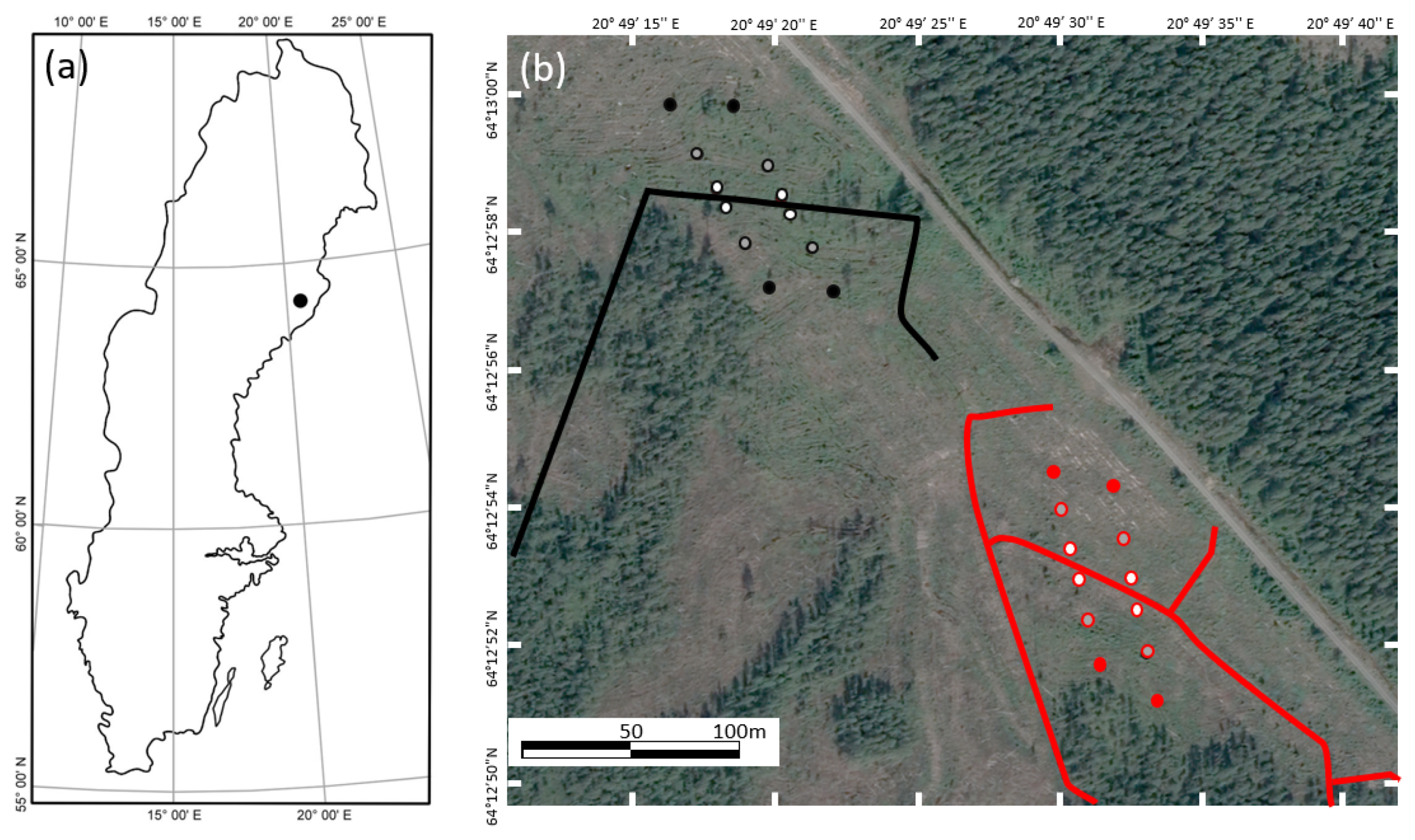
2.1. Site Description and Experimental Design

This study was conducted at a forest clear-cut site (“the Pettersson site” 64°12′56″ N, 20°49′32″ E, 60 m.a.s.l.) located approximately 3 km north of Robertsfors town in the county of Västerbotten, Sweden. The local climate according to the Köppen–Geiger classification [34] is characterized as boreal (Dfc; also called subarctic) with persistent snow cover during ~6 months. According to the data from the nearest weather stations (Brände and Bjuröklubb, 15 km and 46 km from the site, respectively) of the Swedish Meteorological and Hydrological Institute (SMHI; www.smhi.se, accessed on 1 February 2022), the 30-year (1991–2020) mean annual temperature (Recorded in Bjuröklubb) is 4.0 °C, and the mean annual precipitation (Recorded in Brände) is 701 mm, of which about 35% falls as snow.

While detailed Records for the timing of the original drainage and plantation of the former stand are missing, historical air photos suggest that trees and the ditch network of the study site already existed during the early 1960s. Prior to harvest in October 2016, the former stand had a tree volume of 274 m³ ha⁻¹ and consisted of about 75% pine (Pinus sylvestris L.), 22% Norway spruce (Picea abies L.) and 3% broad-leaved tree species (e.g., Betula spp). Soil preparation by mounding was conducted across the entire site in August 2018, followed by the establishment of tree seedlings in June 2019, which consisted of 30% Norway spruce and 70% pine, planted with density of 2100 plants per hectare.

The drainage ditch network is composed of two main ditches that diverge water into different directions, i.e., south-east and south-west (Figure 1). In January 2020, DC was performed along the ditch network branch draining towards the south-east (its surrounding area is hereafter referred to as the DC area), using a tracked excavator. During DC, both vegetation and deposited material were removed from the ditches and piled up along both sides of the ditches. After DC, the open ditches had a trapezoidal shape, with a depth of about 1 m and a width of about 0.5 at the bottom and towards 2 m at the top. The ditch network branch draining to the south-western side was left uncleaned (hereafter referred to as the control area) and characterised by stagnant surface waters due to sediment deposition and vegetation in-growth, which reduced its drainage functions.

The site is located in a region where Podzol is the dominant soil type (Geological Survey of Sweden (SGU)), with soil layers consisting of thin incoherent surface layers of postglacial sand and gravel, while finer soil particles of clay and silt are dominant at 0.5 m below the ground surface. The thin organic layer at our study site was partly mixed into the upper mineral soil layer by the harvest machinery, which resulted in elevated carbon and nitrogen concentrations of 25.1 ± 5.3 % and 0.84 ± 0.19 % (i.e., C:N ratio: 31 ± 1.5) in the 0 to 10 cm profile, respectively. In comparison, carbon and nitrogen content decreased to 10.6 ± 4.5 % and 0.40 ± 0.17 % (i.e., C:N ratio: 31 ± 1.1), respectively, within 10 and 20 cm depth. There was no significant difference in carbon and nitrogen concentrations between the control and DC areas based on the soil samples taken from 24 measurement plots in August 2018. The main herbaceous plant species that were established across the site during the study years following harvest included Deschampsia flexuosa L., Trichophorum alpinum L., Epilobium angustifolium L., Potentilla erecta L., Vaccinium myrtillus L. and Vaccinium vitis-idaea L.

The experimental design included two parallel transects (about 30 m apart) in each of the two treatment areas with sampling plots at three distances (4, 20, and 40 m) on both sides of the ditch along each transect (i.e., 2 treatment areas × 2 transects × 3 distances × 2 sides = 24 plots) (Figure 1). The 40 m plots were also at similar distance to the surrounding intersecting ditches (Figure 1). Pre-treatment data were collected for two years (2018–2019) followed by two years (2020 and 2021) of measurements after the ditch was cleaned in the designated DC treatment area. This experimental setup allowed us to control for potential confounding effects from both spatial (e.g., topography) and temporal (e.g., weather patterns) factors.

2.2. Greenhouse Gas Flux Measurements

We conducted CO₂ and CH₄ flux measurements using the closed dynamic chamber method [35]. The measurements were carried out during daytime in approximately biweekly intervals during the snow-free period (May to October) from 2018 to 2021. In May 2018, square aluminium frames (48.5 × 48.5 cm) with a frame base down to 5 cm below the soil surface were permanently installed at each plot. The observed vegetation species and coverage within the frames were consistent with the surrounding area indicated in Section 2.1 over the study years.

Forest-floor CO₂ and CH₄ fluxes were determined by placing a chamber connected in a closed loop to a portable GHG analyser (Gas Scouter G4301, Picarro Inc., Santa Clara, CA, USA) onto the pre-installed frames. The Gas Scouter has a built-in sampling pump circulating air between chamber and analyser at a flow rate of 0.001 m³ min⁻¹, and Records CO₂ and CH₄ concentrations at a frequency of approximately ~1 Hz, with precision levels of ±150 ppb and ±0.8 ppb, respectively. In the first two years (2018/19), we used a transparent chamber with the dimensions of 48.5 × 48.5 × 30 cm. During the subsequent two years (2020/21), a taller transparent chamber (48.5 × 48.5 × 50 cm) was required to cover the growing herbaceous vegetation within the frames. While effective mixing of the chamber headspace was created by the continuous recirculation pump from the analyser in the smaller chamber used in 2018/19, the larger chamber was equipped with a small fan to further support mixing in the larger and more densely vegetated headspace. A comparison of repeated (i.e., within <5 min) fluxes measured with the two different chamber sizes suggested good agreement for CO₂ (r² = 0.95) and CH₄ (r² = 0.58) fluxes, respectively. The lower r² for the CH₄ flux was likely due to the disturbance from the initial measurement, which may have modified the comparatively small CH₄ concentration gradient before the subsequent measurements. The mixing ratios of CO₂ and CH₄ are reported as dry air mole fractions.

During each flux measurement, a transparent chamber was used at first to measure the net ecosystem exchanges for CO₂ (i.e., NEE) and CH₄ during 90–120 s under natural light conditions. After 2 min of venting, the chamber was placed onto the same frame again and covered by an opaque blanket to estimate the CO₂ flux during dark conditions, i.e., ecosystem respiration (Reco). The gross primary productivity (GPP) was then calculated using the difference between NEE and R_eco.

The average rate of the change in the mixing ratios over time ($dC/dt$; ppm s⁻¹) was estimated using simple linear regression over a chosen data range. The flux rate was then calculated based on $dC/dt$ as a function of chamber headspace volume, air temperature and pressure according to the ideal gas law. Poor-quality flux data were eliminated under the criteria of the root-mean-square error (RMSE) and r² of the chosen $dC/dt$. Based on visual examination of the data, CO₂ fluxes with RMSE > 2.5 ppm and r² < 0.90, and CH₄ fluxes with RMSE > 2.5 ppb and r² < 0.90 were removed. These quality control procedures led to the removal of about 2% and 5% of all CO₂ and CH₄ fluxes measured, respectively. The sign convention in this study is such that positive and negative flux values refer to a net source and sink of the GHG, respectively.

We also conducted measurements of N₂O fluxes during early and late August 2020 with static chambers following the methodology described in Appendix A. The results suggested negligible N₂O fluxes of 14 ± 8 µg-N m⁻² h⁻¹ and 18 ± 5 µg-N m⁻² h⁻¹ in the control and DC area, respectively, which accounted for <1.1% of the GHG balance even when accounting for the 298 higher warming potential of N₂O relative to CO₂. We therefore did not include these measurements into the ordinary measurement program.

2.3. Measurements of Abiotic Factors

To investigate the impact of DC on the environmental factors and to explore their relationships with the measured GHG fluxes, we Recorded a suite of environmental variables in parallel during each flux sampling campaign. Specifically, manual WTL measurements were made inside PVC groundwater tubes (Ø = 32 mm external and 26 mm inside, h = 125 cm, 3 mm holes every 2.5 cm) inserted to a depth of 1 m adjacent to each flux measurement frame. Soil moisture within the upper 5 cm was measured at three sides around the frame using a GS3 combined moisture–temperature sensor connected to a handheld data logger (ProCheck, Decagon Devices, Pullman, WA, USA). Soil temperature (T_s) was also Recorded manually next to each frame at 5 and 10 cm depths (T_s5, T_s10). Air temperature (T_a) was measured using two Hobo^® pendant temperature loggers (Onset Computers, Bourne, MA, USA). One was placed at 2 m height above surface and shaded from direct sunlight, Recording data at 15 min intervals continuously over the year, whereas the other one was operated in the chamber headspace at 5 s intervals during chamber closures. Photosynthetically active radiation (PAR) was continuously measured using two Hobo^® pendant radiation sensors with built-in loggers (Onset Computers, Bourne, MA, USA). Specifically, one sensor Recorded PAR at 5 s intervals inside the chamber during the period of a flux measurement, while another sensor was situated at the centre of the study site to log ambient PAR all year round at an hourly interval. Soil temperature at 5 cm and 10 cm depths was also continuously measured with automated TOMST^® TMS-4 sensors (TOMST, Prague, Czech Republic) installed at 6 selected plots, with each located 4 m, 20 m and 40 m from the ditches in both the control and DC areas. The hourly ambient T_a and PAR data served as input for the nonlinear regression models to predict hourly CO₂ fluxes (see Section 2.4).

2.4. Vegetation Characteristics

The growth of the field-layer vegetation within each flux measurement frame was monitored during the measurement years by taking overhead images during each flux measurement campaign. These images were then analysed to derive a vegetation greenness index defined by the green chromatic coordinate ($g_{cc}$) [36,37,38] (Equation (1)).

$$g_{cc}=G/\left(R+G+B\right)$$

(1)

$g_{cc}$ refers to the greenness index from the image taken on the frame; $R$, $G$ and $B$ denote the intensity (0–255) of the red, green and blue image channels. The g_cc values were averaged for each image pixel located within the chamber frame. Based on the overhead images, we also calculated the ground vegetation areal coverage, which is defined as the vertical projection of vegetation onto a unit of land.

In July 2019 and July 2021, the ground vegetation g_cc and areal coverage for the area surrounding the frames were studied by taking overhead images at 12 spots evenly distributed within 15 m radii around each flux measurement frame. The purposes of these measurements were to (1) evaluate if the vegetation cover inside the flux measurement frames was representative of that within the surrounding area and (2) to increase the sample size to test for DC impacts on ground vegetation development.

Continuous measurements of vegetation growth were also made using two phenocams (TimeLapseCam, Wingscapes, Calera, AL, USA) which Recorded images at hourly intervals with a nadir angle of 15° towards a northernly direction. The g_cc and areal coverage calculated from these images were used to calibrate and interpolate the manual overhead images to frame-specific continuous phenology time series. The latter were then used as model input for estimating annual CO₂ flux budgets (see Section 2.4).

2.5. Statistical Analysis

We first applied mixed effect models with repeated measures to test for the significant effects of the DC and distance to ditch treatments on the spatial variation of environmental (i.e., T_a, T_s10, T_s5, SM, WTL, g_cc and vegetation areal coverage) and flux (i.e., GPP, Reco, NEE and CH₄) variables (Figure 2). The statistical models applied were as follows (Equation (2)):

$$y_{ijk}={\mathsf{\beta }}_0+T_j+{\mathsf{\beta }}_{1}d+S_{ij}+{\epsilon }_{ij}$$

(2)

where y_ij denotes the environmental or gas flux variable for sampling occasion i with DC treatment j (j = control or DC); β₀ denotes the overall mean of the environmental or gas flux variable; T_j denotes the fixed effect of DC treatment j; ${\mathsf{\beta }}_1$ denotes the fixed effect of the sensitivity to distance to ditch d; S_ij denotes the random effect of sampling occasion i; ε_ij denotes the random error for sampling occasion i with treatment j. The model takes into account the random effects presenting a covariance structure where correlations decrease with time [39]. Mixed effect models were proven to be robust to various data distributions [40]. We set the statistical error levels to α = 0.05 for the mixed effect models, and the standard error (±SE) of the sample means was used to indicate the level of uncertainty.

Next, since the mixed effect models did not provide information on the associations between environmental and flux variables, we complemented our statistical analysis by conducting a principal component analysis (PCA) with the goal to identify the three-way interactions between the treatments (DC and distance), environmental factors and flux variables (CO₂ and CH₄) (Figure 2). Principal components (PCs) were calculated using the growing season means of the variables from each measurement plot. Separate PCAs were carried out for the datasets from pre-DC and post-DC treatment periods. Variables were normalised by subtracting each value from the mean and dividing by the standard deviation before inputting them to the PCA models [41]. Significant PCs were selected and presented using the Kaiser criterion [42]. The correlation coefficients (loadings) of the variables with the significant PCs were compared to identify the relationships among variables [43]. All statistical analyses were conducted using the Mathworks Matlab software R2021a.

2.6. Modelling of Annual CO₂ and CH₄ Flux Budgets

Nonlinear regression models following [36,44,45,46] were used to predict hourly and annual R_eco and GPP fluxes based on data of T_a, PAR and g_cc. Particularly, GPP from each frame was fitted to hourly PAR and frame-specific g_cc data using a hyperbolic PAR function adjusted by normalised frame-specific $g_{cc}$ representing seasonal variations in vegetation biomass (Equation (3)):

$$GP{P}_{\left(hr,frame\right)}=\left(\alpha \times P_{max}\times PAR\times g_{c{c}_{\mathrm{norm}}}\right)/\left(\alpha \times PAR+P_{max}\times g_{c{c}_{\mathrm{norm}}}\right)$$

(3)

where GPP denotes the hourly gross primary production (mg m⁻² h⁻¹ of CO₂-C); α denotes the initial slope of quantum use efficiency of photosynthesis (mg µmol photons⁻¹ of CO₂-C); PAR denotes the mean of hourly photosynthetically active radiation (µmol m⁻² s⁻¹); P_max denotes the maximum photosynthesis under infinite PAR (mg m⁻² h⁻¹ of CO₂-C); and $g_{c{c}_{\mathrm{norm}}}$ is the daily frame-specific chromatic greenness index (g_cc) surrounding the frames normalised to the scale of 0 to 1.

Hourly estimates of R_eco were modelled using an exponential function of soil temperature based on [47] adjusted by the normalised frame-specific $g_{cc}$ (Equation (4)):

$$R_{ec{o}_{\left(hr,frame\right)}}=R_0\times ex{p}^{b\times T_{s5}}+\left(\beta \times g_{c{c}_{\mathrm{norm}}}\right)\times ex{p}^{b\times T_{s5}}$$

(4)

where R_eco denotes hourly ecosystem respiration (mg m⁻² h⁻¹ of CO₂-C); $R_0$ denotes soil respiration at 0 °C (mg m⁻² h⁻¹ of CO₂-C); T_s5 denotes soil temperature at 5 cm depth (°C); $b$ denotes the sensitivity of R_eco to T_s5; and β is a scaling parameter associated with the contribution of autotrophic respiration (R)_a to R_eco. Hourly estimates of GPP and R_eco were then summed up for the entire year, and annual NEE was estimated by the difference of the modelled annual GPP and R_eco.

To increase the robustness of the models, we pooled the available data to develop models based on the two pre-DC (2018/19) and two post-DC (2020/21) years separated for the control and DC areas, respectively. The model parameters of the final models selected based on the highest R² are summarised in

Table 1. Model parameters for estimating gross primary production (GPP) (Equation (3)) and ecosystem respiration (R_eco) (Equation (4)) for control and ditch cleaning (DC) clear-cut area, applied separately in the pre-DC years (2018/19) and post-DC years (2020/21); α is the initial slope of the light-use photosynthetic efficiency (mg µmol⁻¹ photons of CO₂-C); $P_{\max }$ is the maximum photosynthetic rate at light saturation (mg m⁻² h⁻¹ of CO₂-C); $R_0$ is respiration rate (mg m⁻² h⁻¹ of CO₂-C) at 0 °C; b is the sensitivity of R_eco to soil temperature (T_s); β represents the contribution of autotrophic respiration to R_eco; numbers in parentheses indicate standard error; R² denotes the coefficient of determination of the model. Number of observations ranges between 186 and 272 for the development of each model.

Time	Pre-DC (2018/19)		Post-DC (2020/21)
Area	Control Area	DC Area	Control Area	DC Area
GPP Model
α	−1.3 (0.37)	−1.1 (1.06)	−4.3 (0.72)	−6.9 (2.1)
$P_{\max }$	−1069 (141)	−1250 (215)	−1589 (74)	−1774 (110)
Adjusted R2	0.47	0.35	0.66	0.58
Reco model
$R_0$	34.9 (5.8)	28.2 (4.2)	47.4 (4.9)	57.5 (6.3)
b	0.09 (0.01)	0.12 (0.01)	0.09 (0.01)	0.05 (0.01)
β	72.9 (21.3)	23.9 (7.7)	86.1 (12.8)	288 (35)
Adjusted R2	0.59	0.65	0.65	0.69

. It is noteworthy that despite similar greenness and areal cover (Table S1), the P_max in the GPP model and the β in the R_eco model were higher in the DC plots during the post-DC period compared to the control plots. This is explained by the greater vascular biomass noted in the DC plots (based on visual observation) at which the same greenness and areal coverage facilitate higher photosynthetic rate compared to moss-dominated ground vegetation. During the snow period, R_eco was represented by R_o, which is an iterated parameter in the respiration model that describes the respiration rate when soil temperature was at 0 °C. The modelled GPP values were zero in response to the negligible exposure of ground vegetation during snow coverage (i.e., $g_{c{c}_{\mathrm{norm}}}$ = 0; Equation (3)).

The uncertainty of the annual CO₂ flux budgets derived by the model extrapolations was evaluated using Monte Carlo simulations. For that purpose, we assigned a normal distribution to each model input parameter (see Table 1) in accordance with its mean and standard deviation derived during model development [48]. Then, a large number (1000) of random draws were taken from the normal distributions of each model parameter. The standard deviation for the set of 1000 predicted estimates was then used to define the uncertainty of the annual CO₂ flux budgets.

Due to the weak relationship between CH₄ fluxes and environmental variables, annual CH₄ balances were interpolated from the median of measured CH₄ fluxes. We propagated the standard errors to estimate the uncertainty of the annual CH₄ budgets due to spatial variability among sampling plots. A baseline winter CH₄ emission rate was estimated based on the assumption that the low CH₄ fluxes Recorded from the late October measurement campaigns (see Section 3.2) continued during the following winter period (i.e., November–April).

3. Results

3.1. Environmental Data

The annual mean air temperature at the nearby SMHI weather station in Bjuröklubb (46 km from the study site) was close to the 30-year average (4.0 °C in 1991–2020) in 2018 (4.4 °C), 2019 (3.9 °C) and 2021 (4.1 °C), but considerably warmer in 2020 (5.9 °C) due to an unusually warm winter period (−0.4 °C and −2.1 °C in January and February, with reference to 30-year average of −5.1 °C and −6 °C). The annual total precipitation in 2018 and 2019 at the nearby SMHI weather station in Brände (15 km from the study site) was 505 and 652 mm, which was lower than the 30-year long-term average (1991–2020) of 701 mm. In the post-DC years of 2020 and 2021, the annual total precipitation was 958 and 1007 mm, substantially higher than the long-term average.

T_a Recorded during the flux measurement campaigns ranged from a minimum of 5.9 ± 0.4 °C during the beginning or the end of the growing season to a maximum of 29.1 ± 1.3 °C in June or July during the four years (Figure 3a). T_s5 and T_s10 measured during flux measurements ranged from 4.4 ± 0.3 °C to 19.3 ± 0.9 °C and from 4.7 ± 0.4 °C to 16.2 ± 0.7 °C, respectively, for the four years (Figure 3a). The difference in T_s5 and T_s10 between the control and DC areas was <0.4 °C during the study years. T_s5 and T_s10 at 4 m distance from the ditch were 0.2 to 0.9 °C lower than at 40 m from the uncleaned ditches in the control area (Table S1). The magnitudes and temporal dynamics of PAR were similar during the study years (Figure 3b).

There was no clear seasonal pattern on the WTL fluctuation, but a shallower WTL was usually observed at the beginning or the end of the growing season. In 2018, the mean WTL averaged over all flux plots and sampling campaigns was −39 ± 2 cm and −43 ± 3 cm in the control and DC areas, respectively (Figure 3c). Thus, the mean WTL was already 5 cm higher in the control area than in the DC area during the pre-DC period. In 2019, the mean WTL rose to −27 ± 1 cm in the control area and −32 ± 1 cm in the DC area, suggesting a significant (p < 0.05) but similar increase in both areas during the second pre-DC treatment year (Table S1). After DC, the mean WTL in the control area rose to −19 ± 1 cm in 2020 and −15 ± 1 cm in 2021, whereas the WTL in the DC area remained at a similar level of −37 ± 2 cm in 2020 and −32 ± 1 cm in 2021, relative to the pre-DC year of 2019. Thus, following DC, the WTL in the DC area was 18 ± 2 cm and 17 ± 2 cm lower than in the control area in 2020 and 2021, respectively. This implies that the WTL difference between the two areas increased by 12 ± 2 cm due to the DC effect. In the control area, significantly shallower WTL was observed in the plots closer to the ditch during all four study years. In the DC area, however, plots closer to the ditch were already characterised by deeper WTL in the pre-DC years, and this spatial difference remained significant in the post-DC years (Table S1).

Similar spatial and temporal patterns were observed for the soil moisture content. Specifically, in the first two pre-treatment years, the annual mean soil moisture remained in the range of 0.29 to 0.36 m³ m⁻³ in the two treatment areas (Figure 3d; Table S1). The difference between the control and DC area increased substantially in the two post-DC years, where in the control area, the soil moisture increased to 0.44 ± 0.02 and 0.43 ± 0.01 m³ m⁻³ in the year 2020 and 2021. In the DC area, the soil moisture remained at 0.30 ± 0.01 and 0.26 ± 0.01 m³ m⁻³ in the year 2020 and 2021, respectively, and was not statistically different from the pre-DC period. Altogether, the DC effect on soil moisture content was estimated at 0.12 m³ m⁻³ based on the additional differences noted between the control and DC areas after DC. The effect of distance to ditches on the soil moisture was similar to its effect on the WTL, with soil moisture decreasing with distance to ditches in the control area but increasing with distance to ditches in the DC area during all measurement years.

In July 2019 and 2021, the seasonal maxima of the greenness index and vegetation areal coverage were not significantly different between the two treatment areas (Figure 4). Averaged over all frames and treatments, the greenness index increased from 0.24 ± 0.02 in July 2019 to 0.53 ± 0.04 in July 2021, while the areal coverage increased from 0.21 ± 0.04 in July 2019 to 0.54 ± 0.05 in July 2021. In the surrounding area, the maximum greenness index and areal coverage over all treatment plots increased from 0.22 ± 0.01 to 0.46 ± 0.02 and from 0.20 ± 0.02 to 0.57 ± 0.02, respectively, over the two years. The greenness index and vegetation areal coverage in the surrounding area at the 4 m distance from the ditch locations were, however, 15% and 30% greater in the control area than in the DC area in July of 2019 and 2021, whereas no difference between both areas was noted at the 20 m and 40 m plots (Table S1). Furthermore, the greenness index and vegetation areal coverage of frames and their surrounding areas agreed well overall, except the greenness index in the frame was 16% greater (p = 0.047) than in the surrounding areas in the DC area in July 2021. In the model extrapolation for annual gas balances, this difference was accounted for by developing treatment-specific models (see Section 2.4).

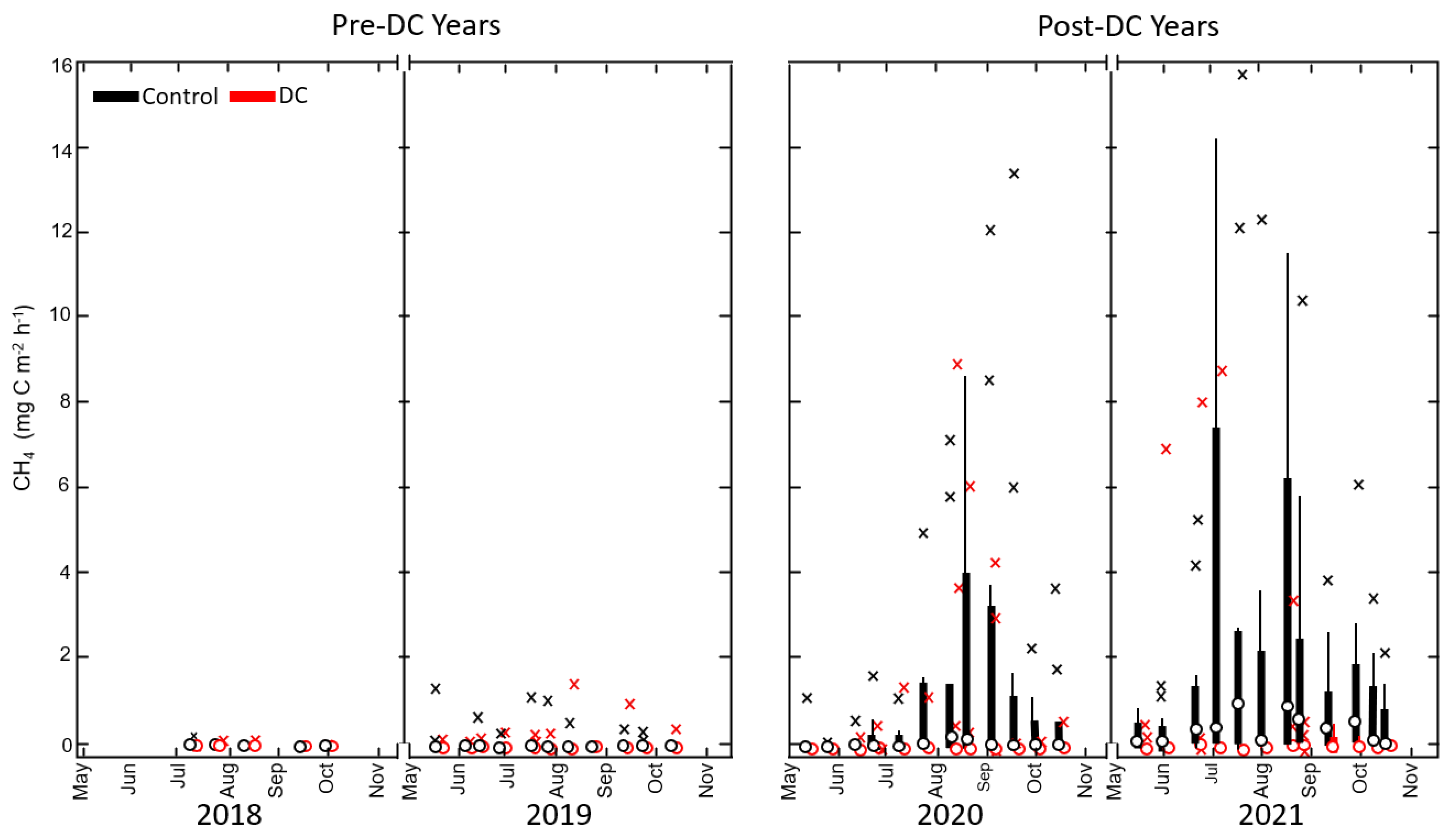
3.2. Temporal Variations of CO₂ and CH₄ Fluxes

The magnitudes and seasonal variations of daytime net CO₂ exchange (NEE) and its components (GPP and R_eco) increased throughout the four measurement years in both the control and DC areas. When averaged over all plots, the instantaneous daytime NEE switched from net emissions of 72 ± 9 mg C m⁻² h⁻¹ in 2018 to a net uptake of 168 ± 27 mg C m⁻² h⁻¹ in 2021 (Figure 5a;

Table 2. Annual central estimates ± standard error (SE) and mixed effect model results for ditch treatment effects (control versus DC) and distance to ditch combinations (4 m, 20 m and 40 m) on CO₂ and CH₄ fluxes based on observations during pre-DC (2018/19) and post-DC periods (2020/21). Mean and median values were applied for the central estimates of CO₂ and CH₄ flux values, respectively. Fixed factors of mixed effect models include ditch cleaning treatment (T), distance to ditches (D) and their interaction (TD). Column N refers to the sample size of each model. Significant p values (α = 0.05) are represented in bold face.

Gas Species	Period	N	Central Estimates ± SE								p Values from the Mixed Effect Models
			Control Area			All Control Plots	DC Area			All DC Plots
			4 m	20 m	40 m		4 m	20 m	40 m		T	D
CO2 (mg C m−2 h−1)
NEE	Pre DC	395	−10 ± 13	87 ± 12	96 ± 9	58 ± 7	66 ± 12	75 ± 13	30 ± 15	57 ± 8	0.75	0.10
	Post DC	577	−157 ± 26	−118 ± 25	3 ± 19	−90 ± 14	−37 ± 25	−156 ± 39	−133 ± 32	−109 ± 19	0.37	0.16
Reco	Pre DC	395	177 ± 17	168 ± 16	121 ± 10	155 ± 8	167 ± 14	168 ± 14	133 ± 9	156 ± 7	0.78	<0.01
	Post DC	577	277 ± 19	296 ± 20	239 ± 17	271 ± 10	302 ± 21	368 ± 23	282 ± 18	317 ± 12	<0.01	0.02
GPP	Pre DC	395	−187 ± 20	−81 ± 15	−25 ± 7	−97 ± 10	−101 ± 19	−94 ± 15	−103 ± 18	−99 ± 10	0.94	<0.01
	Post DC	577	−433 ± 34	−414 ± 31	−235 ± 26	−360 ± 18	−340 ± 37	−525 ± 49	−418 ± 43	−427 ± 25	<0.01	0.02
CH4 (mg C m−2 h−1)
	Pre DC	392	0.00 ± 0.02	−0.03 ± 0.03	−0.02 ± 0.01	−0.02 ± 0.01	−0.04 ± 0.01	−0.03 ± 0.01	−0.02 ± 0.1	−0.03 ± 0.01	0.24	0.85
	Post DC	567	1.2 ± 0.4	0.08 ± 0.3	−0.03 ± 0.01	0.08 ± 0.9	−0.07 ± 0.01	−0.04 ± 0.01	−0.03 ± 0.2	−0.05 ± 0.06	<0.01	<0.01

). From 2018 to 2021, the peak growing season GPP increased about 13 times in the DC area, relative to a 10-time increase in the control area (Table 2). Similarly, daytime measurements of R_eco increased by more than three times in the DC area from 2018 to 2021, whereas in the control area, the increase was by about two times.

In the two pre-treatment years, CH₄ fluxes varied within the 10–90 percentile range of −0.06 to +0.07 mg C m⁻² h⁻¹ across all plots, with a median of −0.02 mg C m⁻² s⁻¹, indicating the majority of fluxes were negative (i.e., uptake) at the site (Figure 6). Occasional emission spikes were observed at individual plots across both the experimental areas throughout the four years (Figure 6). In the two years after DC, the number and magnitude of CH₄ emission spikes increased, particularly during the peak season in both the control and DC areas, but with considerably higher ranges and frequencies observed in the control area. Specifically, the 10–90 percentile ranged from −0.07 to 3.6 mg C m⁻² s⁻¹ in the control area and from −0.14 to 0.11 mg C m⁻² s⁻¹ in the DC area during the two years after DC. The median CH₄ flux was 0.08 mg C m⁻² s⁻¹ in the control area and −0.05 mg C m⁻² s⁻¹ in the DC area (Table 2). It is further noteworthy that most emission spikes were Recorded at the plots 4 m from the uncleaned ditch in the control area, with median emissions of 1.2 mg C m⁻² s⁻¹ (Table 2).

3.3. DC Effect on CO₂ and CH₄ Fluxes

During the pre-treatment period, the mixed effect models suggested that the growing season means of daytime NEE exhibited no significant differences (p > 0.05) between the control and DC areas. The growing season means of the measured GPP and R_eco fluxes also did not differ significantly (p > 0.05) between the two treatment areas during the two pre-treatment years. After DC, both measured R_eco and GPP became significantly (p < 0.01) greater as compared to the control area. Due to similar changes in R_eco and GPP, however, NEE was not significantly affected by DC (p > 0.05).

The mixed effect models indicate no significant difference (p > 0.05) in CH₄ fluxes between the control and DC areas before the treatment (Table 2). In the two years after DC, emissions from the control area became significantly higher (p < 0.01) than from the DC area, consistent with the increased emission spikes in the control area.

3.4. Distance to Ditch Effect Effects on CO₂ and CH₄ Fluxes

The distance to ditches had contrasting effects on NEE, R_eco and GPP. Specifically, NEE shifted from a net CO₂ sink to a net CO₂ source with increasing distance to ditches in the control area, whereas the magnitude of net CO₂ uptake decreased with distance to ditches in the DC area (Table 2). This spatial pattern persisted throughout all four measurement years. Meanwhile, the significant effects of distance to ditches on R_eco and GPP were only noted in the control area, suggesting a decrease in their magnitude with increasing distance to the ditches. In the DC area, however, the highest R_eco and GPP values were observed at 20 m from the ditch (Table 2). These distance effects were consistent throughout all measurement years.

As the CH₄ emission spikes were concentrated at the plots 4 m from the uncleaned ditches, the mixed effect models also suggest a negative effect of distance to ditch on the CH₄ fluxes. However, additional inspection of the data suggests that this distance to ditch effect was mainly driven by a strong gradient in the control area, where CH₄ emissions, coinciding with highest WTL, remained highest at the plots closest (4 m) to ditches.

3.5. Three-Way Interaction between Ditch Treatments, Environmental Factors and GHG Fluxes

The PCA on all variables Recorded during the pre-DC years showed that in total, 83% of the total variance was explained by five significant PCs (Table S3). Together, the first two most significant PCs explained 52% of the total variance (Figure 7). PC1 revealed that vegetation growth (g_cc and areal coverage) was most strongly coherent with the CO₂ component fluxes of R_eco and GPP. Vegetation variables were also positively related to soil carbon and nitrogen content and negatively related to soil temperature. PCA results further showed that R_eco and GPP were negatively associated with the distance to ditch and CN ratios. CH₄ flux had a strong positive connection with WTL and soil moisture in both PC1 and 2 but was not associated with the distance to ditch. During the pre-DC years, the DC treatment variable had relatively small variable loadings in both PC1 and 2, implying that pre-DC environmental conditions and fluxes were comparable between the two measurement areas.

During the post-DC years, 80% of the total variance was explained by four significant PCs (Table S3), while together, the first two most significant principal components explained 54% of the total variance (Figure 7). Compared to the pre-DC years, the DC treatment effect had a larger association with the environmental and flux variables, as reflected by the increased variable loadings in the first two PCs. Specifically, the DC treatment was associated with lower soil moisture, lower WTLs and with increased soil temperature, in correspondence with lower CH₄ fluxes. In contrast, the CO₂ component fluxes were independent from the DC effects on soil temperature and moisture levels but instead were primarily controlled by vegetation growth. The latter also remained positively related to soil carbon and nitrogen contents. The results further show that soil moisture, WTL and thereby CH₄ emissions decreased with greater distance from the ditches. Meanwhile, the small loading of distance to ditch indicated its limited association with the other environmental and CO₂ flux variables relative to the pre-DC period.

3.6. Total Annual Carbon and GHG Balances

Our model estimates suggest that our study site was an annual source of carbon during the four study years, regardless of the DC treatment (Figure 8; Table S2). However, the source magnitude decreased by 78% and 74% in the control and DC areas, respectively, from 6.1 ± 1.2 t-C ha⁻¹ year⁻¹ and 7.2 ± 1.6 t-C ha⁻¹ year⁻¹ in 2018 to 13.1 ± 1.4 t-C ha⁻¹ year⁻¹ and 14.4 ± 1.4 t-C ha⁻¹ year⁻¹ in 2021. The reduction in the net CO₂ emission occurred because GPP (from zero to −12.1 ± 0.7 t-C ha⁻¹ year⁻¹) increased more than R_eco (from 6.6 ± 1.4 t-C ha⁻¹ year⁻¹ to 13.8 ± 1.1 t C ha⁻¹ year⁻¹) between 2018 to 2021 in both areas. The interannual variations in the modelled annual CO₂ flux components were similar between the control and DC treatment areas over the four years. Averaged over the four study years, there was no significant difference between the model estimates of annual NEE in the control and DC areas.

The interannual variations in the modelled annual CH₄ balance over the four years differed between the control and DC treatment areas. Specifically, in the control area, the annual CH₄ flux increased from −2.2 to 27 kg C ha⁻¹ year⁻¹ between 2018 and 2021. Within the control area, the observed CH₄ emissions at 4 m from the uncleaned ditches were by 1 and 2 magnitudes higher relative to the 20 and 40 m locations, respectively, leading to a contribution of 6% and 25% to the carbon balance at this location in 2020 and 2021, respectively. In the DC area, however, the inter-annual variation in the CH₄ balance was relatively small and stable within a range of −3.0 to −2.3 kg-C ha⁻¹ year⁻¹_, which represented < 0.15% of the total carbon balances in all four study years. However, when considering the global warming potential of CH₄ as 86 times higher relative to CO₂ over a 20-year time frame (IPCC, 2014), the median contribution of CH₄ to the annual GHG budget (in t CO₂-eq ha⁻¹ year⁻¹) increased from 0.1% in 2018 to 39% in 2021 in the control area, but remained within <5% in the DC area, respectively. The enhanced CH₄ emissions resulted in a 23% increase in the total annual GHG emissions in the control area in 2021; however, given the large uncertainty (from the spatial variation) associated with the annual CH₄ flux estimate, the total annual GHG balances were not significantly different between the control and DC areas.

4. Discussion

4.1. Ditch Cleaning Effects on Hydrology, Vegetation and GHG Fluxes

This study investigated DC’s effects on CO₂ and CH₄ fluxes in a two-way experimental set up, i.e., through (i) a direct comparison of fluxes in the control and DC area, respectively, and (ii) a pre- versus post-treatment assessment in the DC area. Both evaluation alternatives indicated only a minor effect of DC on the net CO₂ exchange and its component fluxes GPP and R_eco. Instead, both spatial and temporal variations were mainly dependent on the within-site variations in herbaceous ground vegetation during the post-harvest years. The similar spatial pattern of herbaceous ground vegetation before and after DC indicated the minor impact of DC on the ground vegetation development. In addition, GPP and R_eco were strongly correlated with variations in soil carbon and nitrogen, which is in line with previous studies suggesting that soil fertility and organic content are the primary controls over spatial variations of CO₂ fluxes [49,50]. This is because the decomposition of organic matter and associated nutrient release are tightly coupled to microbial respiration and plant carbon uptake [51]. Essentially, positive feedback may develop as the increased plant growth provides additional organic matter input, thereby speeding up the carbon cycle [50]. The spatial variations in both ground vegetation together with soil carbon and nitrogen at our study site itself did not correspond to DC effects and instead might be a relict of the historical drainage effects and/or disturbance during harvest and site preparation.

The lack of WTL changes in the DC area after DC appeared surprising at first. However, this could be explained by the increase in precipitation during the post-DC years, which may have counterbalanced the enhanced drainage function following DC. In fact, the concurrent rise in WTL (by 14 cm) in the control area reveals an increased drainage function in the DC area during the two post-DC years. Given the wetter conditions, the control area was characterised by a relatively shallow WTL (−17 cm on average) during these two post-harvest years, resulting in a narrow upper oxic zone which likely supressed decomposition and the growth of vascular plants, thus explaining the limited R_eco and GPP noted in the control area during these wet years (Table 2). However, we observed no significant correlation between WTL and CO₂ flux components (i.e., R_eco and GPP) during periods when WTL was <−20 cm, which agrees with similar findings from a peatland forest clear-cut in boreal Finland [26]. This indicates that DC’s effects on the Reco, GPP and NEE largely depend on both the initial WTL and the effectiveness of the DC, which jointly regulate the change in soil surface oxic conditions and subsequently the production and decomposition of organic content in the initial years following harvest.

Contrary to our expectations, we did not observe a clear pattern in the effect of ditch distance on WTL, soil moisture and CO₂ fluxes. Given the constantly shallow WTL conditions (−17 cm on average during the two post-harvest years) at all distances from uncleaned ditches, the R_eco and GPP were higher at locations closer to these uncleaned ditches, which could be due to the contribution from the more extensive growth of Sphagnum moss under the wet conditions. In the DC area, however, the highest R_eco and GPP values observed at 20 m from the cleaned ditches may have resulted from optimum WTLs of −35 to −40 cm that created a favourable balance between sufficient water and oxygen availability for enhancing vascular plant growth and decomposition processes [52,53]. Such an impact could have dominated over the drainage legacy effects, as observed in the control area with limited WTL variations. Since the year-to-year increase in GPP was greater than that of R_eco at 20 m from the cleaned ditches, the most negative measured daytime NEE (−156 ± 39 mg C m⁻² h⁻¹) indicates that such a WTL condition likely favours net CO₂ uptake. Nevertheless, we cannot rule out the possibility that the high rainfall during both post-DC years may have influenced the moisture condition and eventually the locations where the optimal WTL with highest fluxes were observed. Thus, additional observations during dry years will be required to further elucidate the interactions among ditch distance, soil water levels and CO₂ fluxes.

CH₄ fluxes are known to be strongly related to soil oxic conditions [54,55] and thus are likely modified by a reduction in WTL following DC. Specifically, the deeper mean WTL of −35 ± 2 cm in the DC area retained a substantial surface oxic layer and thereby provided favourable conditions for CH₄ oxidation while limiting CH₄ production to the deeper soil layer [26]. In comparison, the majority (75%) of plots in the control area, including all plots at 4 m distance from the ditches, were characterised by relatively high WTL (between 0 and −20 cm) and close to saturated soil conditions (> 0.45 m³ m⁻³), which may have facilitated large CH₄ production and emissions from the enhanced anaerobic soil layer [26,56,57]. However, it is noteworthy that CH₄ emission spikes occurred more frequently at several DC plots given the same or even deeper WTL during the two post-DC years. This is likely due to the enhanced amount of vascular ground vegetation (e.g., Deschampsia flex spp.) noted in these DC plots, with roots reaching deep into the CH₄ production zone, providing substrate from root exudates to methanogens and supporting the plant-mediated transport of CH₄ into the atmosphere [58,59,60]. Alternatively, more frequent rain events might have resulted in additional CH₄ production from waterlogged microsites within the oxic soil layer [61]. Altogether, these findings highlight that, relative to the CO₂ exchange, CH₄ fluxes were more sensitive to DC via its effects on soil hydrological properties and plant growth.

4.2. Ditch Cleaning Effects on the Annual C and GHG Balances of a Boreal Forest Clear-Cut

We observed a rapid decrease in annual carbon emissions during the four measurement years, which indicates that the high emissions commonly expected to occur in boreal clear-cuts [26,62] might be limited to only the initial few years. One reason for this decrease was the rapid development of the herbaceous ground vegetation, which resulted in increasing GPP. The importance of the fast Recovery of ground vegetation was previously highlighted in nutrient-poor boreal forest clear-cuts on mineral soils [63,64,65]. In comparison, the increase in R_eco over the four years was relatively smaller, possibly because the wet conditions in 2020/21 might have constrained microbial aerobic decomposition. Previous studies have shown that the Recovery rate of the net carbon balance after clear-cutting depends on regeneration management, biomass production and decomposition rate, suggesting that it could take anywhere between 1 and 20 years for GPP to counterbalance R_eco [62,66,67,68,69].

Despite the higher daytime R_eco and GPP measured in the DC area, our model estimates of their annual sums were not different between the two experimental areas during both post-DC years. The apparent discrepancy in the treatment effect between the modelled annual sums relative to the instantaneous daytime measurements is explained by the greater vegetation coverage in the surrounding area compared to the measurement frames in the control treatment (Figure 4). While the measured fluxes corresponded to the vegetation coverage within the frames, the vegetation coverage in the surrounding area was used as input in the model extrapolation with the goal to obtain estimates that were representative of the entire area. The higher vegetation coverage in the surrounding control area relative to the DC area was primarily a result of the higher prevalence of Sphagnum moss species under favourable shallow WTL conditions. We note that our results are confined to the initial vegetation responses after DC, whereas continued vascular species and seedling development will likely result in a greater contribution from plant carbon uptake to the total respiration at the DC area in the future.

Our result that CH₄ had a minor (<2.5%) contribution to the total carbon balance is in agreement with several previous studies conducted in other boreal forest clear-cuts on drained mineral soils [62,63,70] as well as with findings from peatland forest clear-cuts [26]. However, in terms of the total GHG balance where, the GWP of CH₄ is 86 times over CO₂, CH₄ emissions become increasingly important when the CO₂ balance is closer towards carbon neutral, i.e., during the later phase when the site shifts from an annual source to sink (Figure 7). Leaving the ditches uncleaned might further create local hotspots for CH₄ emission within the waterlogged areas near the ditch. In comparison, DC effectively mitigated CH₄ emissions by maintaining low WTLs deeper than −30 cm during the wet post-harvest years, resulting in even slightly negative (i.e., uptake) annual GHG balance. This is in agreement with a previous study suggesting that post-harvest CH₄ emissions increase only if the WTL rises above approximately −20 cm [65]. It is noteworthy that the modelled annual CH₄ flux sums were characterised by considerable uncertainty due to the high spatial variability inherent to our measurement plots. The use of the eddy covariance technique is required to overcome this challenge and to provide more precise estimates for the CH₄ balance of heterogeneous clear-cut areas [71].

We caution that our study lacked flux data from the snow-covered winter periods, and our annual flux budget therefore relied on simple assumptions for estimating the contribution from winter fluxes. However, previous studies based on continuous year-round data collected with the eddy covariance and automated chamber techniques suggest low fluxes during snow-covered winter periods commonly contributing to less than 10% of the annual CO₂ and CH4 budgets in boreal ecosystems [62,72,73]. This indicates a limited potential bias introduced by our assumptions in estimating the winter flux. It is further noteworthy that this study only addressed the initial responses of the environment and fluxes to DC. However, long-term effects on the growth of the tree layer might further enhance the DC impact on the forest carbon balance over an entire rotation period. Moreover, the ditch functions will again deteriorate over time through erosion and sedimentation, which may result in a nonlinear trajectory of DC effects on the soil water dynamics and thus carbon balance. Thus, more empirical data from winter periods and extending over the decadal timescale of post-DC years are required to better understand the DC effects on the forest ecosystem carbon balance across contrasting sites. Given the steady increase in DC activities, particularly within Fennoscandia, it is essential to improve our knowledge of DC effects on the forest ecosystem–atmosphere exchange of carbon and GHGs with the goal to provide an empirical knowledge base that can support the development of sustainable and climate-responsible forest management strategies.

5. Conclusions

This study investigated how the cleaning of degraded drainage ditches affects CO₂ and CH₄ fluxes from a drained forest clear-cut on mineral soil in boreal Sweden over four years (i.e., 2–5 years after harvest). Based on our findings, we conclude that:

(1)

The clear-cut area with old and degraded ditches acted as a net carbon source in all four post-harvest years. However, during the study period, the annual total carbon emissions decreased by 76% (from 6.7 ± 1.4 t-C ha⁻¹ year⁻¹ to 1.6 ± 1.6 t-C ha⁻¹ year⁻¹).

(2)

Ditch cleaning had a limited initial effect on the spatio-temporal variations in the net CO₂ exchange and its component fluxes, GPP and R_eco. The variation in the component fluxes was instead primarily controlled by the within-site variations in ground vegetation development, likely in response to drainage legacy effects on soil carbon and nitrogen contents.

(3)

In comparison, ditch cleaning reduced the soil water content and thereby mitigated CH₄ emissions during wet post-harvest years.

(4)

Ditch distance had no consistent effect on CO₂ and CH₄ fluxes. While R_eco and GPP tended to increase towards uncleaned ditches coinciding with legacy trends in soil carbon and nitrogen content, maximum R_eco and GPP occurred at 20 m from cleaned ditches, likely in response to an optimal WTL for vascular plants commonly observed in the DC area. In comparison, high emissions of CH₄ mainly occurred on nearly saturated soil locations near to uncleaned ditches.

(5)

Overall, ditch cleaning had no significant impact on the annual carbon and GHG balance in the initial post-harvest years.

(6)

There is a critical need for long-term observations to evaluate DC effects on the forest carbon and GHG balances during the entire subsequent rotation period.

References

1. Bradshaw, C.J.; Warkentin, I.G. Global estimates of boreal forest carbon stocks and flux. Glob. Planet. Chang. 2015, 128, 24–30. [Google Scholar] [CrossRef]
2. Lindeskog, M.; Smith, B.; Lagergren, F.; Sycheva, E.; Ficko, A.; Pretzsch, H.; Rammig, A. Accounting for forest management in the estimation of forest carbon balance using the dynamic vegetation model LPJ-GUESS (v4. 0, r9710): Implementation and evaluation of simulations for Europe. Geosci. Model Dev. 2021, 14, 6071–6112. [Google Scholar] [CrossRef]
3. Paavilainen, E.; Päivänen, J. Utilization of peatlands. In Peatland Forestry; Springer: Berlin/Heidelberg, Germany, 1995; pp. 15–29. [Google Scholar] [CrossRef]
4. Fenton, N.J.; Bergeron, Y. Facilitative succession in a boreal bryophyte community driven by changes in available moisture and light. J. Veg. Sci. 2006, 17, 65–76. [Google Scholar] [CrossRef]
5. Simard, M.; Lecomte, N.; Bergeron, Y.; Bernier, P.Y.; Paré, D. Forest productivity decline caused by successional paludification of boreal soils. Ecol. Appl. 1997, 17, 1619–1637. [Google Scholar] [CrossRef]
6. Skaggs, R.W.; Tian, S.; Chescheir, G.M.; Amatya, D.M.; Youssef, M.A. Forest drainage. In Forest Hydrology: Processes, Management and Assessment; CABI: Oxfordshire, UK, 2016; pp. 124–140. [Google Scholar]
7. Dubé, S.; Plamondon, A.P.; Rothwell, R.L. Watering up after clear-cutting on forested wetlands of the St. Lawrence lowland. Water Resour. Res. 1995, 31, 1741–1750. [Google Scholar] [CrossRef]
8. Roy, V.; Ruel, J.C.; Plamondon, A.P. Establishment, growth and survival of natural regeneration after clearcutting and drainage on forested wetlands. For. Ecol. Manag. 2000, 129, 253–267. [Google Scholar] [CrossRef]
9. Koivusalo, H.; Ahti, E.; Laurén, A.; Kokkonen, T.; Karvonen, T.; Nevalainen, R.; Finér, L. Impacts of ditch cleaning on hydrological processes in a drained peatland forest. Hydrol. Earth Syst. Sci. 2008, 12, 1211–1227. [Google Scholar] [CrossRef]
10. Manninen, P. Effects of forestry ditch cleaning and supplementary ditching on water quality. Boreal Environ. Res. 1998, 3, 23–32. [Google Scholar]
11. Ahti, E.; Kojola, S.; Nieminen, M.; Penttilä, T.; Sarkkola, S. The effect of ditch cleaning and complementary ditching on the development of drained Scots pine-dominated peatland forests in Finland. In Proceedings of the 13th International Peat Congress. After Wise Use—The Future of Peatlands, Tullamore, Ireland, 8–13 June 2008; pp. 457–459. [Google Scholar]
12. Ahti, E.; Päivänen, J. Response of stand growth and water table level to maintenance of ditch networks within forest drainage areas. In Northern Forested Wetlands: Ecology and Management; CRC Press: Boca Raton, FL, USA, 2018; pp. 449–457. ISBN 9780203745380. [Google Scholar]
13. Sarkkola, S.; Hökkä, H.; Ahti, E.; Koivusalo, H.; Nieminen, M. Depth of water table prior to ditch network maintenance is a key factor for tree growth response. Scand. J. For. Res. 2012, 27, 649–658. [Google Scholar] [CrossRef]
14. Sikström, U.; Hökkä, H. Interactions between soil water conditions and forest stands in boreal forests with implications for ditch network maintenance. Silva Fennica 2016, 50, 1416. [Google Scholar] [CrossRef] [Green Version]
15. Sikström, U.; Hjelm, K.; Hanssen, K.H.; Saksa, T.; Wallertz, K. Influence of mechanical site preparation on regeneration success of planted conifers in clearcuts in Fennoscandia—A review. Silva Fennica 2020, 54, 10172. [Google Scholar] [CrossRef] [Green Version]
16. Minkkinen, K.; Vasander, H.; Jauhiainen, S.; Karsisto, M.; Laine, J. Post-drainage changes in vegetation composition and carbon balance in Lakkasuo mire, Central Finland. Plant Soil 1999, 207, 107–120. [Google Scholar] [CrossRef]
17. Hökkä, H.; Kojola, S. Kunnostusojituksen kasvureaktioon vaikuttavat tekijät [Factors affecting growth response due to ditch network maintenance operation]. In Suometsien Kasvatuksen ja Käytön Teemapäivät [Management and Utilization of Peatland Forests]; NBN:fi-metla-2014112610063; Hiltunen, I., Kaunisto, S., Eds.; The Finnish Forest Research Institute: Vantaa, Finland, 2001; Volume 832, pp. 30–36. (In Finnish) [Google Scholar]
18. Hökkä, H.; Kojola, S. Suometsien kunnostusojitus—Kasvureaktion tutkiminen ja kuvaus. [Ditch network maintenance in peatland forests—Growth response and it’s description]. In Soilla ja Kankailla—Metsien Hoitoa ja Kasvatusta Pohjois-Suomessa [On Peatlands and Uplands—Forest Management in Northern Finland]; Jortikka, S., Varmola, M., Tapaninen, S., Eds.; The Finnish Forest Research Institute: Vantaa, Finland, 2003; Volume 903, ISBN 951-40-1897-4. (In Finnish) [Google Scholar]
19. Lauhanen, R.; Ahti, E. Effects of maintaining ditch networks on the development of Scots pine stands. Suo 2001, 52, 29–38. [Google Scholar]
20. Houle, D.; Lajoie, G.; Duchesne, L. Major losses of nutrients following a severe drought in a boreal forest. Nat. Plants 2016, 2, 1–5. [Google Scholar] [CrossRef]
21. Verry, E.S. Hydrological processes of natural, northern forested wetlands. In Northern Forested Wetlands; Routledge: New York, NY, USA, 1997; pp. 163–188. ISBN 9780203745380. [Google Scholar]
22. Jutras, S.; Plamondon, A.P.; Hökkä, H.; Bégin, J. Water table changes following pRecommercial thinning on post-harvest drained wetlands. For. Ecol. Manag. 2006, 235, 252–259. [Google Scholar] [CrossRef]
23. Leppä, K.; Korkiakoski, M.; Nieminen, M.; Laiho, R.; Hotanen, J.P.; Kieloaho, A.J.; Korpela, L.; Laurila, T.; Lohila, A.; Minkkinen, K.; et al. Vegetation controls of water and energy balance of a drained peatland forest: Responses to alternative harvesting practices. Agric. For. Meteorol. 2020, 295, 108198. [Google Scholar] [CrossRef]
24. Marcotte, P.; Roy, V.; Plamondon, A.P.; Auger, I. Ten-year water table Recovery after clearcutting and draining boreal forested wetlands of eastern Canada. Hydrol. Processes Int. J. 2008, 22, 4163–4172. [Google Scholar] [CrossRef]
25. Drzymulska, D. Peat decomposition-shaping factors, significance in environmental studies and methods of determination; a literature review. Geologos 2016, 22, 61–69. [Google Scholar] [CrossRef] [Green Version]
26. Korkiakoski, M.; Tuovinen, J.P.; Penttilä, T.; Sarkkola, S.; Ojanen, P.; Minkkinen, K.; Rainne, J.; Laurila, T.; Lohila, A. Greenhouse gas and energy fluxes in a boreal peatland forest after clear-cutting. Biogeosciences 2019, 16, 3703–3723. [Google Scholar] [CrossRef] [Green Version]
27. Borken, W.; Davidson, E.A.; Savage, K.; Sundquist, E.T.; Steudler, P. Effect of summer throughfall exclusion, summer drought, and winter snow cover on methane fluxes in a temperate forest soil. Soil Biol. Biochem. 2006, 38, 1388–1395. [Google Scholar] [CrossRef]
28. Feng, H.; Guo, J.; Han, M.; Wang, W.; Peng, C.; Jin, J.; Song, X.; Yu, S. A review of the mechanisms and controlling factors of methane dynamics in forest ecosystems. For. Ecol. Manag. 2020, 455, 117702. [Google Scholar] [CrossRef]
29. Fest, B.; Hinko-Najera, N.; von Fischer, J.C.; Livesley, S.J.; Arndt, S.K. Soil methane uptake increases under continuous throughfall reduction in a temperate evergreen, broadleaved Eucalypt forest. Ecosystems 2017, 20, 368–379. [Google Scholar] [CrossRef]
30. Minkkinen, K.; Laine, J. Vegetation heterogeneity and ditches create spatial variability in methane fluxes from peatlands drained for forestry. Plant Soil 2006, 285, 289–304. [Google Scholar] [CrossRef]
31. Hånell, B.; Magnusson, T. An evaluation of land suitability for forest fertilization with biofuel ash on organic soils in Sweden. For. Ecol. Manag. 2005, 209, 43–55. [Google Scholar] [CrossRef]
32. Kayes, I.; Mallik, A. Boreal Forests: Distributions, Biodiversity, and Management; Springer International Publishing: Cham, Germany, 2020; pp. 1–12. [Google Scholar] [CrossRef]
33. Liski, J.; Westman, C.J. Carbon storage in forest soil of Finland. 2. Size and regional pattern. Biogeochemistry 1997, 36, 261–274. [Google Scholar] [CrossRef]
34. Kottek, M.; Grieser, J.; Beck, C.; Rudolf, B.; Rubel, F. World map of the Köppen-Geiger climate classification updated. Meteorol. Z. 2006, 15, 259–263. [Google Scholar] [CrossRef]
35. Livingston, G.P.; Hutchinson, G.L. Enclosure-based measurement of trace gas exchange: Applications and sources of error. Biog. Trace Gases Meas. Emiss. Soil Water 1995, 51, 14–51. [Google Scholar]
36. Järveoja, J.; Peichl, M.; Maddison, M.; Soosaar, K.; Vellak, K.; Karofeld, E.; Teemusk, A.; Mander, Ü. Impact of water table level on annual carbon and greenhouse gas balances of a restored peat extraction area. Biogeosciences 2016, 13, 2637. [Google Scholar] [CrossRef] [Green Version]
37. Peichl, M.; Sonnentag, O.; Nilsson, M.B. Bringing color into the picture: Using digital repeat photography to investigate phenology controls of the carbon dioxide exchange in a boreal mire. Ecosystems 2015, 18, 115–131. [Google Scholar] [CrossRef]
38. Sonnentag, O.; Hufkens, K.; Teshera-Sterne, C.; Young, A.M.; Friedl, M.; Braswell, B.H.; Milliman, T.; O’Keefe, J.; Richardson, A.D. Digital repeat photography for phenological research in forest ecosystems. Agric. For. Meteorol. 2012, 152, 159–177. [Google Scholar] [CrossRef]
39. Phillips, R.L.; Whalen, S.C.; Schlesinger, W.H. Influence of atmospheric CO2 enrichment on nitrous oxide flux in a temperate forest ecosystem. Glob. Biogeochem. Cycles 2001, 15, 741–752. [Google Scholar] [CrossRef]
40. Schielzeth, H.; Dingemanse, N.J.; Nakagawa, S.; Westneat, D.F.; Allegue, H.; Teplitsky, C.; Réale, D.; Dochtermann, N.A.; Garamszegi, L.Z.; Araya-Ajoy, Y.G. Robustness of linear mixed-effects models to violations of distributional assumptions. Methods Ecol. Evol. 2020, 11, 1141–1152. [Google Scholar] [CrossRef]
41. Jolliffe, I.T. Principal component analysis: A beginner’s guide—I. Introduction and application. Weather 1990, 45, 375–382. [Google Scholar] [CrossRef]
42. Kaiser, H.F. The application of electronic computers to factor analysis. Educ. Psychol. Meas. 1960, 20, 141–151. [Google Scholar] [CrossRef]
43. Cadima, J.; Jolliffe, I.T. Loading and correlations in the interpretation of principle compenents. J. Appl. Stat. 1995, 22, 203–214. [Google Scholar] [CrossRef]
44. Järveoja, J.; Peichl, M.; Maddison, M.; Teemusk, A.; Mander, Ü. Full carbon and greenhouse gas balances of fertilized and nonfertilized reed canary grass cultivations on an abandoned peat extraction area in a dry year. Gcb Bioenergy 2016, 8, 952–968. [Google Scholar] [CrossRef]
45. Kandel, T.P.; Elsgaard, L.; Karki, S.; Lærke, P.E. Biomass yield and greenhouse gas emissions from a drained fen peatland cultivated with reed canary grass under different harvest and fertilizer regimes. BioEnergy Res. 2013, 6, 883–895. [Google Scholar] [CrossRef]
46. Olson, D.M.; Griffis, T.J.; Noormets, A.; Kolka, R.; Chen, J. Interannual, seasonal, and retrospective analysis of the methane and carbon dioxide budgets of a temperate peatland. J. Geophys. Res. Biogeosci. 2013, 118, 226–238. [Google Scholar] [CrossRef]
47. Lloyd, J.; Taylor, J.A. On the temperature dependence of soil respiration. Funct. Ecol. 1994, 8, 315–323. [Google Scholar] [CrossRef]
48. Smith, J.E.; Heath, L.S. Identifying influences on model uncertainty: An application using a forest carbon budget model. Environ. Manag. 2001, 27, 253–267. [Google Scholar] [CrossRef]
49. Allison, S.D.; Treseder, K.K. Warming and drying suppress microbial activity and carbon cycling in boreal forest soils. Glob. Chang. Biol. 2008, 14, 2898–2909. [Google Scholar] [CrossRef] [Green Version]
50. Hobbie, S.E.; Nadelhoffer, K.J.; Högberg, P. A synthesis: The role of nutrients as constraints on carbon balances in boreal and arctic regions. Plant Soil 2002, 242, 163–170. [Google Scholar] [CrossRef]
51. Piirainen, S.; Finér, L.; Mannerkoski, H.; Starr, M. Carbon, nitrogen and phosphorus leaching after site preparation at a boreal forest clear-cut area. For. Ecol. Manag. 2007, 243, 10–18. [Google Scholar] [CrossRef]
52. Silvola, J.; Alm, J.; Ahlholm, U.; Nykaenen, H.; Martikainen, P.J. The contribution of plant roots to CO2 fluxes from organic soils. Biol. Fertil. Soils 1996, 23, 126–131. [Google Scholar] [CrossRef]
53. Lafleur, P.M.; Hember, R.A.; Admiral, S.W.; Roulet, N.T. Annual and seasonal variability in evapotranspiration and water table at a shrub-covered bog in southern Ontario, Canada. Hydrol. Processes Int. J. 2005, 19, 3533–3550. [Google Scholar] [CrossRef]
54. Martikainen, P.J.; Nykänen, H.; Alm, J.; Silvola, J. Change in fluxes of carbon dioxide, methane and nitrous oxide due to forest drainage of mire sites of different trophy. Plant Soil 1995, 168, 571–577. [Google Scholar] [CrossRef]
55. Roulet, N.T.; Ash, R.; Quinton, W.; Moore, T. Methane flux from drained northern peatlands: Effect of a persistent water table lowering on flux. Glob. Biogeochem. Cycles 1993, 7, 749–769. [Google Scholar] [CrossRef] [Green Version]
56. Ojanen, P.; Minkkinen, K.; Alm, J.; Penttilä, T. Soil–atmosphere CO2, CH4 and N2O fluxes in boreal forestry-drained peatlands. For. Ecol. Manag. 2010, 260, 411–421. [Google Scholar] [CrossRef]
57. Ojanen, P.; Minkkinen, K.; Penttilä, T. The current greenhouse gas impact of forestry-drained boreal peatlands. For. Ecol. Manag. 2013, 289, 201–208. [Google Scholar] [CrossRef]
58. Gauci, V.; Gowing, D.J.; Hornibrook, E.R.; Davis, J.M.; Dise, N.B. Woody stem methane emission in mature wetland alder trees. Atmos. Environ. 2010, 44, 2157–2160. [Google Scholar] [CrossRef] [Green Version]
59. Terazawa, K.; Ishizuka, S.; Sakata, T.; Yamada, K.; Takahashi, M. Methane emissions from stems of Fraxinus mandshurica var. japonica trees in a floodplain forest. Soil Biol. Biochem. 2007, 39, 2689–2692. [Google Scholar] [CrossRef]
60. Korkiakoski, M.; Määttä, T.; Peltoniemi, K.; Penttilä, T.; Lohila, A. Excess soil moisture and fresh carbon input are prerequisites for methane production in podzolic soil. Biogeosciences Discuss. 2021, 19, 2025–2041. [Google Scholar] [CrossRef]
61. Radu, D.D.; Duval, T.P. Impact of rainfall regime on methane flux from a cool temperate fen depends on vegetation cover. Ecol. Eng. 2018, 114, 76–87. [Google Scholar] [CrossRef]
62. Vestin, P.; Mölder, M.; Kljun, N.; Cai, Z.; Hasan, A.; Holst, J.; Klemedtsson, L.; Lindroth, A. Impacts of clear-cutting of a boreal forest on carbon dioxide, methane and nitrous oxide fluxes. Forests 2020, 11, 961. [Google Scholar] [CrossRef]
63. Strömgren, M.; Hedwall, P.O.; Olsson, B.A. Effects of stump harvest and site preparation on N2O and CH4 emissions from boreal forest soils after clear-cutting. For. Ecol. Manag. 2016, 371, 15–22. [Google Scholar] [CrossRef]
64. Sundqvist, E.; Vestin, P.; Crill, P.; Persson, T.; Lindroth, A. Short-term effects of thinning, clear-cutting and stump harvesting on methane exchange in a boreal forest. Biogeosciences 2014, 11, 6095–6105. [Google Scholar] [CrossRef] [Green Version]
65. Uri, V.; Kukumägi, M.; Aosaar, J.; Varik, M.; Becker, H.; Aun, K.; Lõhmus, K.; Soosaar, K.; Astover, A.; Uri, M.; et al. The dynamics of the carbon storage and fluxes in Scots pine (Pinus sylvestris) chronosequence. Sci. Total Environ. 2022, 817, 152973. [Google Scholar] [CrossRef]
66. Hyvönen, R.; Ågren, G.I.; Linder, S.; Persson, T.; Cotrufo, M.F.; Ekblad, A.; Freeman, M.; Grelle, A.; Janssens, I.A.; Jarvis, P.G.; et al. The likely impact of elevated [CO2], nitrogen deposition, increased temperature and management on carbon sequestration in temperate and boreal forest ecosystems: A literature review. New Phytol. 2007, 173, 463–480. [Google Scholar] [CrossRef]
67. Kowalski, A.S.; Loustau, D.; Berbigier, P.; Manca, G.; Tedeschi, V.; Borghetti, M.; Valentini, R.; Kolari, P.; Berninger, F.; Rannik, Ü.; et al. Paired comparisons of carbon exchange between undisturbed and regenerating stands in four managed forests in Europe. Glob. Chang. Biol. 2004, 10, 1707–1723. [Google Scholar] [CrossRef]
68. Rannik, Ü.; Altimir, N.; Raittila, J.; Suni, T.; Gaman, A.; Hussein, T.; Hölttä, T.; Lassila, H.; Latokartano, M.; Lauri, A.; et al. Fluxes of carbon dioxide and water vapour over Scots pine forest and clearing. Agric. For. Meteorol. 2002, 111, 187–202. [Google Scholar] [CrossRef]
69. Rebane, S.; Jõgiste, K.; Põldveer, E.; Stanturf, J.A.; Metslaid, M. Direct measurements of carbon exchange at forest disturbance sites: A review of results with the eddy covariance method. Scand. J. For. Res. 2019, 34, 585–597. [Google Scholar] [CrossRef]
70. Kulmala, L.; Aaltonen, H.; Berninger, F.; Kieloaho, A.J.; Levula, J.; Bäck, J.; Hari, P.; Kolari, P.; Korhonen, J.F.; Kulmala, M.; et al. Changes in biogeochemistry and carbon fluxes in a boreal forest after the clear-cutting and partial burning of slash. Agric. For. Meteorol. 2014, 188, 33–44. [Google Scholar] [CrossRef]
71. Pihlatie, M.; Rinne, J.; Ambus, P.; Pilegaard, K.; Dorsey, J.R.; Rannik, Ü.; Markkanen, T.; Launiainen, S.; Vesala, T. Nitrous oxide emissions from a beech forest floor measured by eddy covariance and soil enclosure techniques. Biogeosciences 2005, 2, 377–387. [Google Scholar] [CrossRef] [Green Version]
72. Chi, J.; Nilsson, M.B.; Kljun, N.; Wallerman, J.; Fransson, J.E.; Laudon, H.; Lundmark, T.; Peichl, M. The carbon balance of a managed boreal landscape measured from a tall tower in northern Sweden. Agric. For. Meteorol. 2019, 274, 29–41. [Google Scholar] [CrossRef]
73. Korkiakoski, M.; Tuovinen, J.P.; Aurela, M.; Koskinen, M.; Minkkinen, K.; Ojanen, P.; Ojanen, P.; Penttilä, T.; Rainne, J.; Laurila, T. Methane exchange at the peatland forest floor–automatic chamber system exposes the dynamics of small fluxes. Biogeosciences 2017, 14, 1947–1967. [Google Scholar] [CrossRef] [Green Version]
Figure 1. (a) Location of the Pettersson study site in boreal Sweden, and (b) map of ditch network at the Pettersson field site. Cleaned and uncleaned ditches are marked in red and black, respectively. The locations for flux measurements at 4 m, 20 m and 40 m distance from the ditch, respectively, are marked in red for the cleaned area and black for uncleaned area.
Forests 13 00842 g001
Figure 2. Flowchart of study methodology.
Forests 13 00842 g002
Figure 3. Environmental variables including (a) air (Ta) and soil temperature (Ts5 at 5 cm and Ts10 at 10 cm depth), (b) photosynthetically active radiation (PAR), (c) water table level (WTL), (d) soil moisture (SM) monitored at the measurement plots (shown as means of 4 m, 20 m and 40 m from ditch) during flux measurements. PAR, WTL and SM data are averaged for each sampling occasion and grouped by experimental area (control versus DC) and year (pre-DC years of 2018 and 2019 with post-DC year of 2020 and 2021). The variable means of each sampling occasion ± standard error (SE) are presented for both control and DC areas (n = 12), respectively.
Forests 13 00842 g003
Figure 4. Ground vegetation greenness index inside the frames and in their surrounding areas within 15 m of each flux measurement plot in July 2019 and in July 2021, grouped by ditch cleaning treatment (control versus DC) and distance to ditches (4 m, 20 m and 40 m). The boxes denote the interquartile range with the median indicated inside each box, whereas the lines extending from the boxes indicate the range of each category. Different letters above boxes (a, b, c) refer to compact letter display of one-way ANOVA that indicate significant differences (α = 0.05) among groups, followed by the least significant difference test.
Forests 13 00842 g004
Figure 5. Seasonal variations of carbon dioxide (CO2) flux components including (a) net ecosystem exchange (NEE), (b) ecosystem respiration (Reco) and (c) gross primary productivity (GPP) in control and ditch-cleaned (DC) clear-cut areas during pre-DC (2018/19) and post-DC periods (2020/21). Positive and negative values represent losses and uptakes by the ecosystem, respectively. The circles denote sample (n = 12) medians, whilst the bottom and top edges of the thick bar indicate the 25th and 75th percentiles. The vertical line denotes the range excluding outliers (crosses), which are defined as the values more than 1.5 interquartile range away from the top or bottom of the line. Data shown represent the means of measurement plots at all distances from ditches.
Forests 13 00842 g005
Figure 6. Seasonal variation of methane (CH4) fluxes in control and ditch cleaning (DC) clear-cut areas during pre-DC (2018/19) and post-DC periods (2020/21). Negative values denote uptake. The circles denote sample (n = 12) medians, whilst the bottom and top edges of the thick bar indicate the 25th and 75th percentiles. The vertical line denotes the range excluding outliers (crosses), which are defined as the values more than 1.5 interquartile range away from the top or bottom of the line. Data shown represent the means across all distances from ditches.
Forests 13 00842 g006
Figure 7. Principal component analysis (PCA) biplots of the first two principal components (PC1 and PC2) based on the plot-averaged measurement data displaying variable loadings and object scores, during (a) pre-DC and (b) post-DC periods. Variable loadings of all other significant PCs are listed in Table S3. Filled symbols denote the component loadings of the measured variables. Crosses highlighted in black (control area) and red (DC area) denote the component scores of each measurement plot. Colour intensity of component scores decreases with the distance to the ditches. Note that ecosystem uptake in NEE and GPP is given a negative sign, resulting in negative correlation to both PC1s despite positive causal relation. Abbreviations represent greenness index (gcc), soil moisture (SM), air temperature (Ta), soil 5 or 10 cm depth temperature (Ts5, Ts10), vegetation areal coverage (VC), water table level (WTL), soil carbon (C) and nitrogen content (N) along with their C:N ratio (CN) for environmental variables (black symbols); net ecosystem exchange (NEE), ecosystem respiration (Reco), gross primary productivity (GPP) and methane (CH4) for flux variables (blue symbols); and DC treatment and distance to ditch variable (purple symbols). Note that the DC variable was fitted as a binary variable for control (0) and DC (1) treatments.
Forests 13 00842 g007
Figure 8. Model estimates for the total annual carbon dioxide (CO2) and methane (CH4) balance (upper panels) and total annual greenhouse gas balance (lower panels) in the control and ditch cleaning treatments areas (DC) during the four study years. CO2 balances comprise the net exchange (NEE) and its component fluxes of gross primary productivity (GPP) and the ecosystem respiration (Reco). Scale of CH4 flux is at 0.1 times scale of CO2 flux (blue axis to the right). Greenhouse gas balance of CO2 and CH4 uses global warming potentials of 86 for CH4 over a 20−year timeframe (IPCC, 2013).
Forests 13 00842 g008