Abstract
Structure-based forest management (SBFM) is a method for improving forest structure and quality based on nearest-neighbor analysis. Stand spatial structure directly affects the health and stability of forest ecosystems. Research on the effects of SBFM on the distribution of spatial structure parameters is needed to provide a scientific basis for further development and implementation of SBFM technology in forestry. The present study was conducted on six permanent plots (20 m × 20 m) established within a Platycladus orientalis (L.) Franco plantation in Beijing, China. Changes in stand spatial structure parameters (SSSPs) were evaluated in managed and control plots at three time points: before SBFM and after 2 and 7 years of SBFM. The results showed that SBFM gradually accelerated the development of the P. orientalis plantation toward a random distribution pattern, reaching a significant difference within 2 years. SBFM promoted the growth of medium and dominant trees, with a significant difference between SBFM and control stands after 7 years. It led to a slight increase in mingling compared to the control, although no significant differences were observed between treatments. SBFM generally decreased the proportions of disadvantageous microstructures (disadvantaged trees with non-randomly distributed, disadvantaged trees with a low degree of mingling, and non-randomly distributed trees with a low degree of mingling). It also improved the ratio of torch (R2) units to dumbbell (R1) units, gradually improving the stability of the plantation forest. The results of this study suggest that SBFM optimized the spatial structure of a P. orientalis plantation in Beijing, China, and was conducive to tree growth and forest stand productivity.
1. Introduction
Forest structure, or the distribution of individual plants and the connection of their attributes, is the most important and fundamental feature of forest ecosystems; it reflects both autogenic developmental processes (including regeneration pattern, competition, and the consequent self-thinning) and past and present disturbance events [1]. Thus, forest structure is both a product and driver of ecosystem processes and biological diversity [2]. It is influenced by extensive interactions among various natural and ecological processes over long spatiotemporal scales [3] and determines the quality of forest ecosystem goods and services [4]. As it affects forest productivity, tree species diversity, and biological habitat, forest structure is an important factor in forest ecosystem analysis and management [5].
Analyzing forest structure is an important component of forest management and contributes to the understanding of forest communities [5]. In this context, forest spatial structure is more important than non-spatial structure because it provides more detailed descriptions, largely determines competition and spatial niches among trees, and reflects the health status, growth potential, and stability of tree stands [6]. Therefore, investigations of forest spatial structure are necessary for understanding characteristics of a forest community and designing forest protection and management strategies.
To date, several methods have been proposed to describe and compare stand spatial structures, including classic methods, nearest-neighbor analysis methods, point pattern analysis, and marked second-order characteristics methods [7,8,9,10,11]. These methods have been widely applied in forestry and ecology. Nearest-neighbor analysis has been used to analyze forest spatial structure, competition, dominance, and species composition. In particular, stand spatial structure parameters (SSSPs), which are based on the spatial relationships among four nearest-neighbor trees, have been used to accurately interpret spatial structure characteristics in forests of various dimensions [12,13,14,15,16,17].
Different management techniques can have varying effects on tree species composition, stand density, and tree size distribution, which can in turn alter forest structure. Reasonable forest management measures based on scientific principles can improve both stand structure and forest quality [17,18,19,20]. Structure-based forest management (SBFM) is a promising forestry management approach based on successful experiments conducted in developed countries, as well as forest management practices in China [21,22,23,24]. SBFM assumes that the system structure determines function and aims to cultivate a healthy, stable, high-quality, high-efficiency forest; it uses structural parameters to guide adjustments and optimize forest structure [5]. Thus, SBFM uses scientific methods to quantify descriptions of forest structure and improve forest quality through changes in species composition and structural diversity. For example, it can be used to transition evenly aged plantations to structurally complex forests or to manage unevenly aged, mixed-species forests [3,13,17,24,25,26].
Platycladus orientalis (L.) Franco is an evergreen coniferous tree species that originates in China and exhibits strong adaptability to climate and stress resistance [27,28]. As it thrives under a wide range of climate and soil conditions, P. orientalis is among the main afforestation tree species in the artificial forests of northern China, where it is valued for its ecological, social, and economic benefits [29,30]. Platycladus orientalis grows on an area of more than 3.5 million ha, with an estimated stocking volume of 0.199 billion m3 [31]. Given the important applications of P. orientalis, previous studies have analyzed its spatial structure [30,32], ecological stoichiometry [28,33], water use [34], understory plant diversity [35], regeneration characteristics [36], and soil properties [37]. Other studies have focused on the effects of different P. orientalis management regimes on understory plant growth and diversity, soil enzymes and nutrients, and scenic quality [38,39,40]. However, little research has been conducted on optimizing spatial structure for P. orientalis plantations. In particular, as management duration has increased, changes to stand spatial structure following SBFM have remained poorly understood, despite the importance of this technique to sustainable forest management. Therefore, we evaluated the effects of SBFM on the spatial structure characteristics of a P. orientalis plantation using SSSPs. The goals of this study were (1) to compare the spatial structure characteristics of a P. orientalis plantation under SBFM and an unmanaged plantation; (2) to understand the dynamic changes in the characteristics of the stand spatial structure in a P. orientalis plantation under SBFM and an unmanaged plantation; (3) to reveal the impact of SBFM on the spatial structure of the P. orientalis plantation. The results contribute to the structural optimization and sustainable development of P. orientalis plantation and provide a scientific basis for cultivating healthy, stable, high-quality P. orientalis plantations.
2. Materials and Methods
2.1. Study Areas
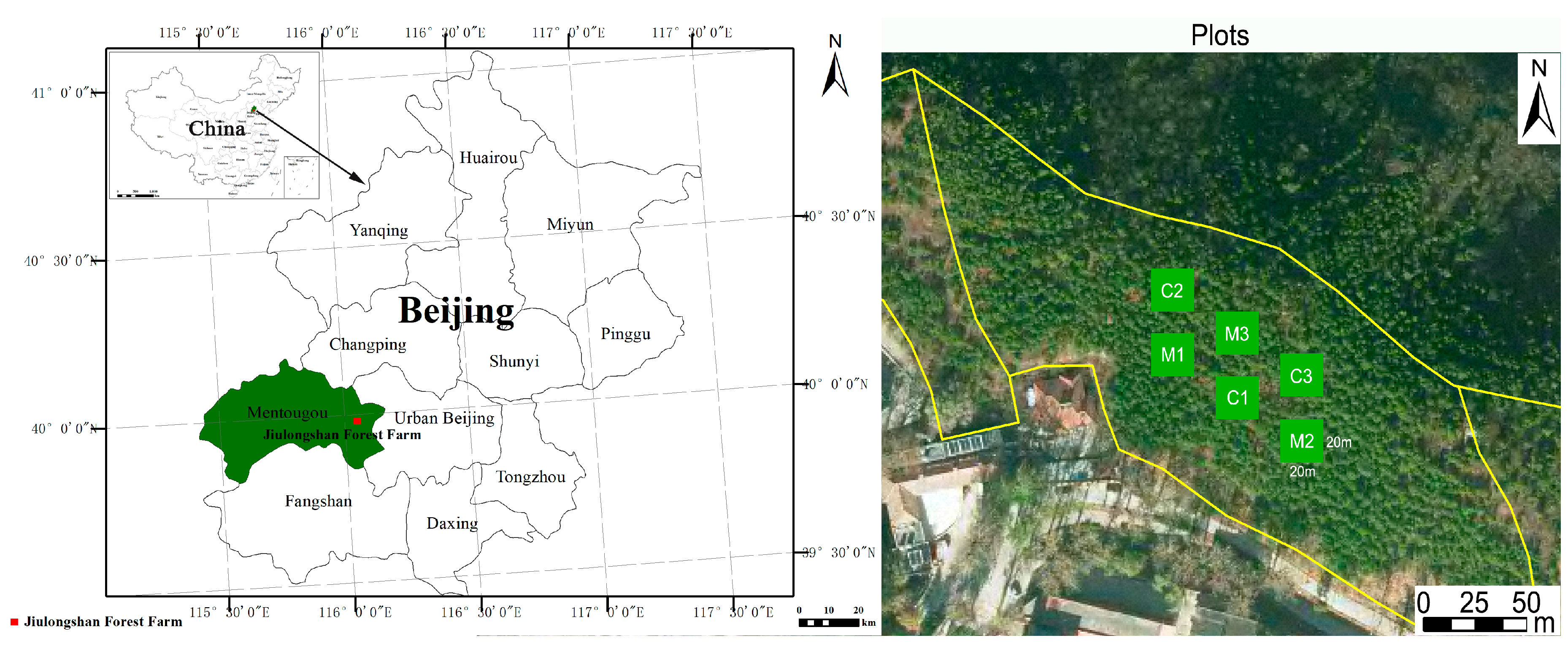
This study was conducted at Jiulongshan Forest Farm in the Jiulong Mountains (115°59′–116°07′ E, 39°54′–39°59′ N; 100–997 m a.s.l.), located near Beijing, east of the Taihang Mountains (Figure 1). The region has a temperate continental climate and is affected by monsoons. The annual average temperature is 11.8 °C. The study region has an annual mean precipitation of 630 mm and an average yearly relative humidity of 66%. Precipitation is uneven throughout the year, with a wet season from June to September and a dry season from October to May. The total evaporation capacity and frost-free period are approximately 1870 mm and 216 days, respectively. The soil is a brown, rocky, mountain forest soil with high stone content, and the average soil layer thickness is 20–50 cm. The topography is steep and undulating, and the main vegetation types are coniferous and broadleaf plantation trees, with P. orientalis, Pinus tabulaeformis, and Quercus variabilis as the dominant species [30,32].
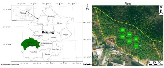
Figure 1.
The study plots, located in Jiulongshan Forest Farm, Mentougou District, Beijing, PR China. Green squares indicate the location and size of plots, and M1-M3 and C1-C3 represent managed and control plots, respectively.
2.2. Study Site and Data Collection
In spring 2013, six plots (20 m × 20 m) were established at Jiulongshan Forest Farm. The location and site conditions of the six plots were nearly identical. All trees with diameters at breast height (DBH) > 5 cm in each plot were positioned with a Topcon GTS602 (Topcon, Tokyo, Japan) autofocus total station. Tree DBH, height, and crown diameter were recorded. To avoid edge effects, we established a 3 m buffer zone in each plot. The basic stand characteristics of the plots are listed in Table 1.

Table 1.
The basic stand characteristics of the plots.
In fall 2013, SBFM began in plots M1–M3; no forestry operations were conducted in control plots C1–C3, which were referred to as CK. After 2 and 7 years of SBFM, in fall 2015 and 2020, respectively, the six plots were surveyed, and the tree DBH, height, and crown diameter of all remaining living trees with DBH > 5 cm were recorded. These values were used to calculate SSSPs.
2.3. Data Analysis
In this study, spatial structure characteristics of a P. orientalis plantation were compared between SBFM and unmanaged plots according to three SSSPs: mingling (), dominance (), and uniform angle index (). is the probability that a reference tree (i) belongs to the same species as its four nearest neighbors (j) (Equation (1)), and it reflects the degree of tree species segregation among tree species. A larger value indicates the presence of more species in the spatial structural unit. describes the size relationship between i and j (Equation (2)) and reflects the degree of DBH differentiation. Larger values indicate that the reference is larger than all four neighbors (dominant). indicates the spatial dispersion of j around i (Equation (3)) and determines the distribution pattern by comparing the included angle formed by any two neighbors and the reference and standard angle () [41]. Larger values indicate more concentrated distribution patterns. SSSPs are graded on a five-point scale (0.00, 0.25, 0.50, 0.75, or 1.00), with each value corresponding to a different stand state; together, they describe the relationships among tree species, size, and distribution within a structural unit consisting of a single reference tree (i) and the four nearest adjacent trees [5]. The SSSP system shows great flexibility for expressing stand structure and is highly sensitive to parameter changes; therefore, it is highly suitable for analyzing stand dynamics over small scales or long time frames [7,42].
By definition, can only represent two possible types of random structural unit in terms of horizontal distribution (). Both subtypes exist simultaneously in all forests. In structural units, two angles are lower than the standard angle (), whereas the other two angles are greater. These four angles have two possible distributions [17,43]:
Type R1: In any two adjacent angles, one is <, and the other is ≥. Thus, for the R1 distribution,
where the corresponding reference trees are R1 random trees. This distribution is also called a “dumbbell” unit (Figure 2), in reference to its shape.
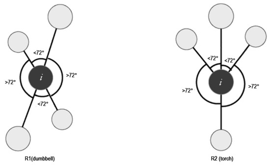
Figure 2.
Two types of random structural unit.
Type R2: Two adjacent angles can be found that are <, whereas the other two angles are ≥. Thus, Equation (3) can be presented as follows:
where the corresponding reference trees are R2 random trees. This distribution is also called a “torch” unit (Figure 2), in reference to its shape.
The proportions of different random structural units were analyzed.
The SSSPs of each tree were calculated with Winkelmass software [44], and the proportions of each random structural unit were analyzed. To avoid edge effects, we set a 3 m buffer, and the average SSSPs for each plot were calculated. All other data analyses and graphics were produced in R v. 4.1.2 (R Development Core Team, Vienna, Austria). One-way analysis of variation (ANOVA) was used to evaluate differences in the relative frequencies of combination with and without SBFM among the three time points: before management and after 2 and 7 years of management. Figures were prepared with the ggplot2 R package [45].
3. Results
3.1. Zero-Variate and Univariate Distributions of SSSPs
3.1.1. Zero-Variate and Univariate Distributions of
All average values were <0.50, and those in the SBFM plots were higher than those in the control plots, regardless of management duration (Table 2). differed significantly between SBFM and the control treatment only after 2 years of management (p < 0.05) (Table 2).
Table 2.
The average values of SSSPs of plots.
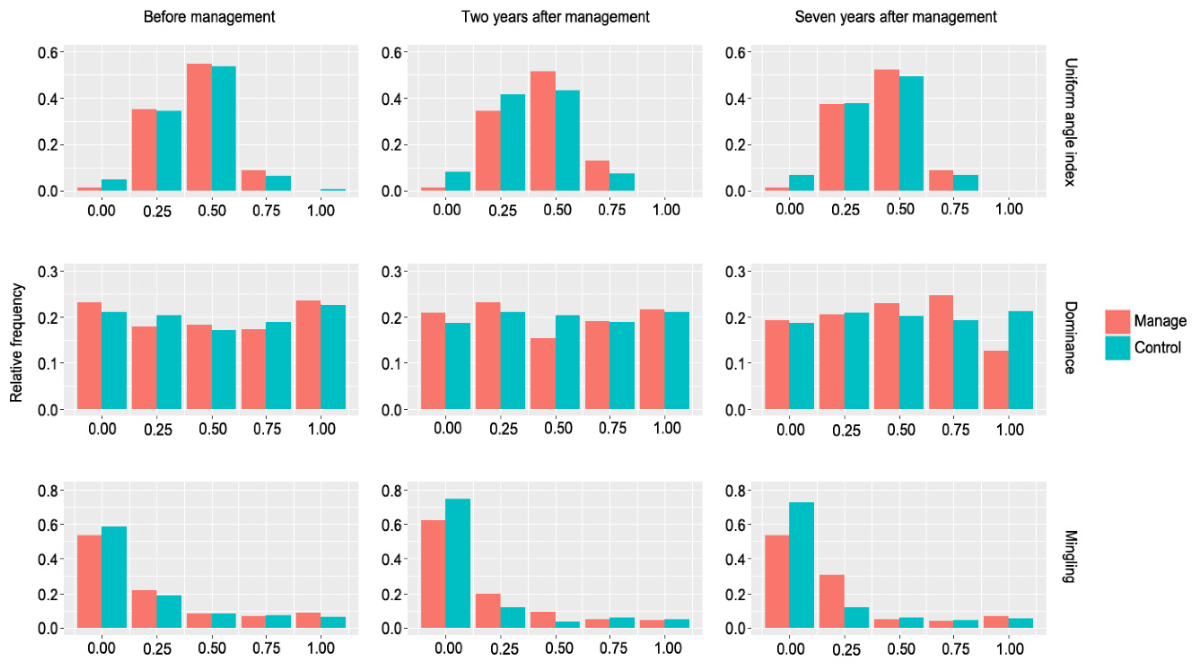
Most trees were randomly distributed in all stands ( = 0.50), and the relative frequency of trees with uniform distribution ( = 0.00, 0.25) decreased in the SBFM plots compared to the control plots. As management duration increased, the proportion of randomly distributed trees was always >50% in the SBFM plots ( = 0.50), whereas in the control plots it gradually decreased to <50%. The proportion of trees that were uniformly distributed ( = 0.00) differed significantly between the SBFM and control stands after 2 years of management (p < 0.05) (Figure 3).
Figure 3.
Frequency distributions of SSSPs at different management years.
3.1.2. Zero-Variate and Univariate Distributions of
Average values were lower in the SBFM plots than in the control plots (Table 2). As management duration increased, average values gradually decreased in the SBFM plots, whereas those in the control plots gradually increased. Average values did not differ significantly between the SBFM and control stands after 2 years of management but differed significantly after 7 years of management (p < 0.05) (Table 2).
Trees in most stands were evenly distributed at each level of dominance, and the relative frequency of trees with a dominant distribution ( = 0.00, 0.25) was higher in the SBFM plots than in the control plots. As management duration increased, the relative frequency of dominant ( = 0.00, 0.25) and medium ( = 0.50) trees in the SBFM plots gradually increased, whereas in the control stands they increased slightly. The relative frequency of medium ( = 0.50) and absolutely disadvantaged ( = 1.00) trees differed significantly between the SBFM and control plots after both 2 and 7 years of management (p < 0.05) (Figure 3). The relative frequency of absolutely disadvantaged ( = 1.00) trees differed significantly between 2 and 7 years of management (p < 0.05).
3.1.3. Zero-Variate and Univariate Distributions of
Average values were <0.25 all plots, with those in the SBFM plots higher than those in the control (Table 2). As management duration increased, the average values of both SBFM and control plots first decreased and then increased (Table 2).
The relative frequency results confirmed that most trees in all stands showed low mixtures ( = 0.00, 0.25) in any management year, with no significant differences between the SBFM and control plots (Figure 3).
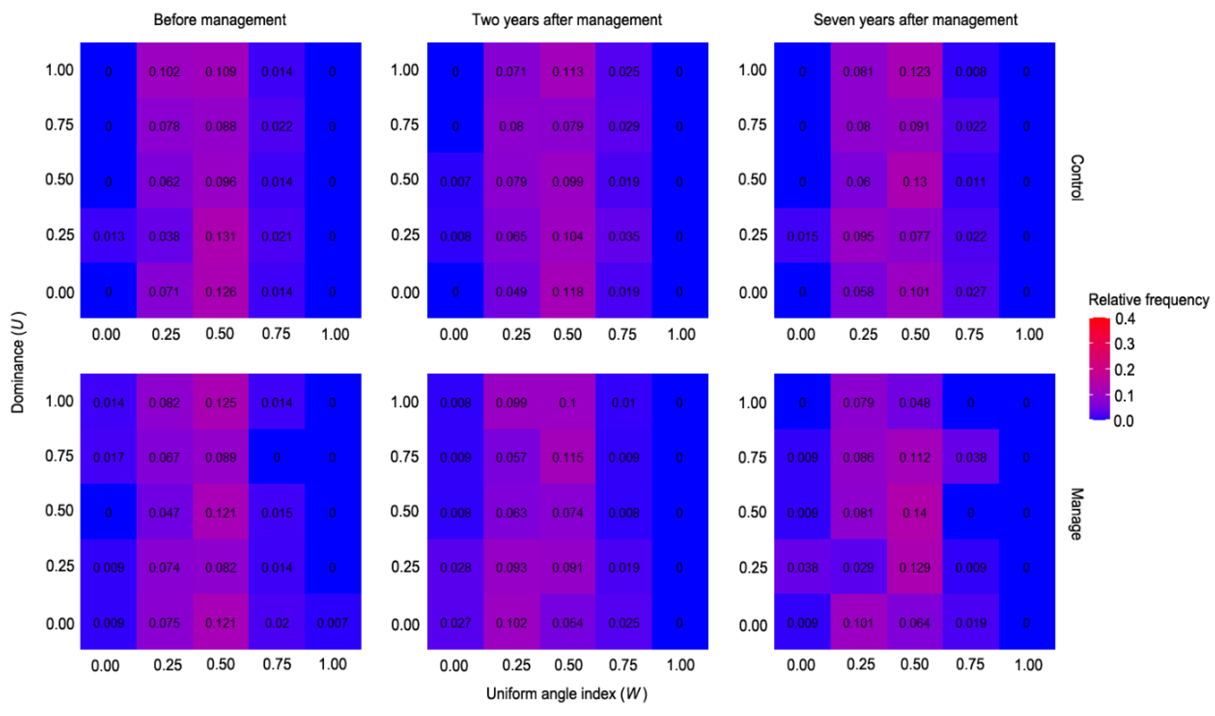
3.2. Bivariate Distributions of SSSPs
3.2.1. -
All stands had similar - index bivariate distributions (Figure 4), which were approximately symmetrical around the random distribution axis ( = 0.50) and declined gradually toward zero on both sides. The frequency of increased with that of and then decreased, suggesting a near-normal distribution. Compared to the combinations for each stand, which had frequency values between 0.000 and 0.038, the frequencies of = 0.50 and 0.25 were remarkably high, accounting for >0.850 of the whole. However, the frequency of trees with a low degree of dominance ( = 0.00, 0.25) and random distribution ( = 0.50) did not differ significantly between the SBFM and control plots in different management years. Significant differences between the SBFM and control plots were greatest for the structural combination = 0.50 and = 0.50, as well as = 1.00 and = 0.50, after 2 and 7 years of management (Figure 4).
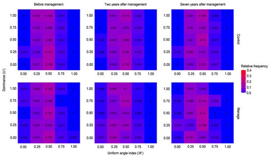
Figure 4.
Bivariate distributions of and at different management years.
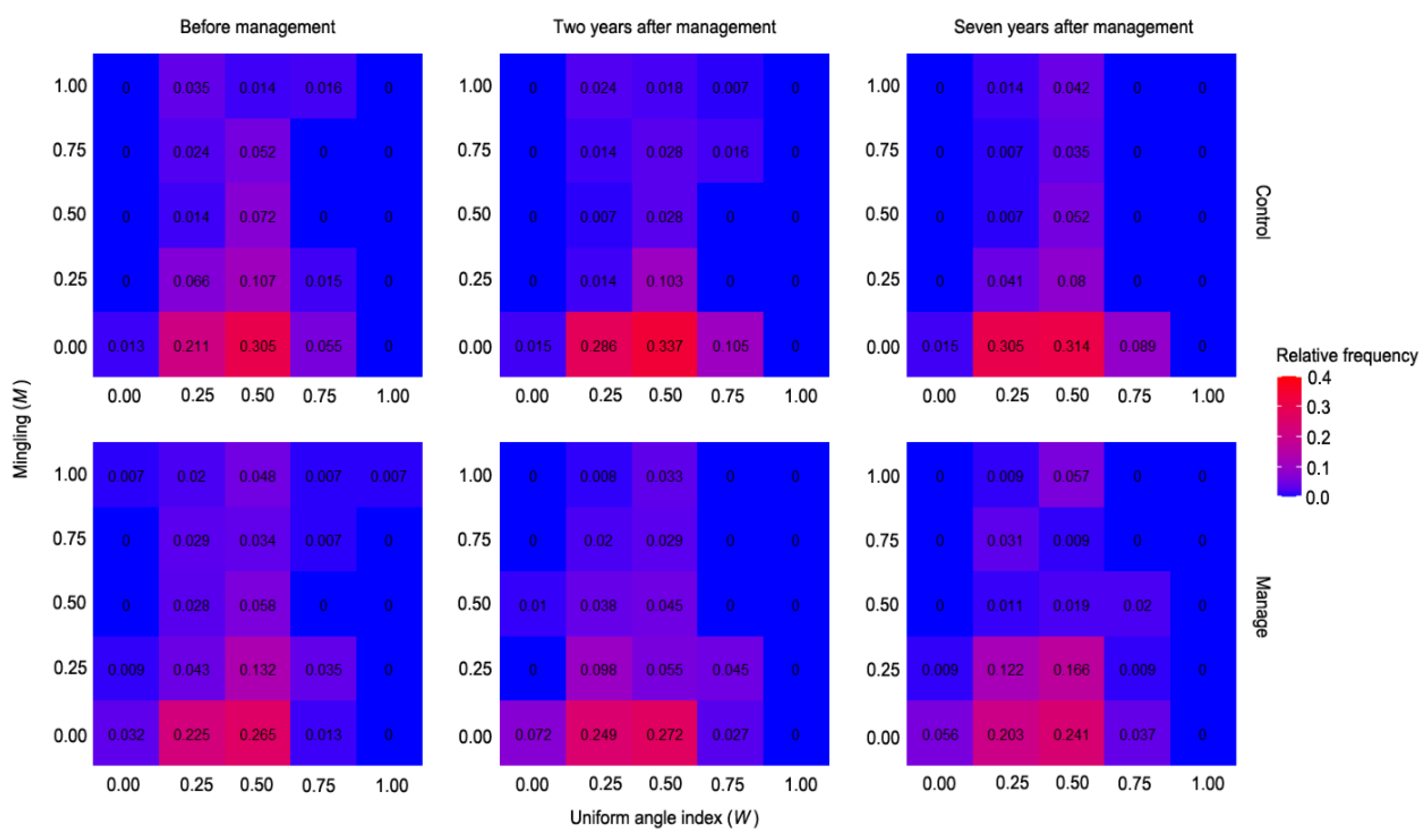
3.2.2. -
Regardless of the type and management years of the stand, the - bivariate distributions (Figure 5) indicated that the highest frequency appeared at = 0.00 at each class. Frequency values for each class first increased and then declined, accompanied by an increase in , which reached its maximum at = 0.50. Meanwhile, the highest pole value in all stands always occurred with the combination = 0.00 and = 0.50, which represented the case in which the reference tree was surrounded by the same species and had a random distribution pattern in the quadrats. In addition, as management duration increased, the relative frequency of trees between SBFM and control stands with the combination of complete mixture ( = 1.00) and a random distribution ( = 0.50) gradually improved, and the corresponding values of SBFM stands were greater than those of control stands. However, compared to the control, the relative frequency of trees in SBFM with no mixture ( = 0.00) and a random distribution ( = 0.50) was reduced, showing 0.305 and 0.265, 0.337 and 0.272, and 0.314 and 0.241 for stands before management, after 2 years of management, and after 7 years of management, respectively (Figure 5).
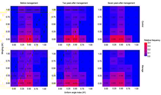
Figure 5.
Bivariate distributions of and at different management years.
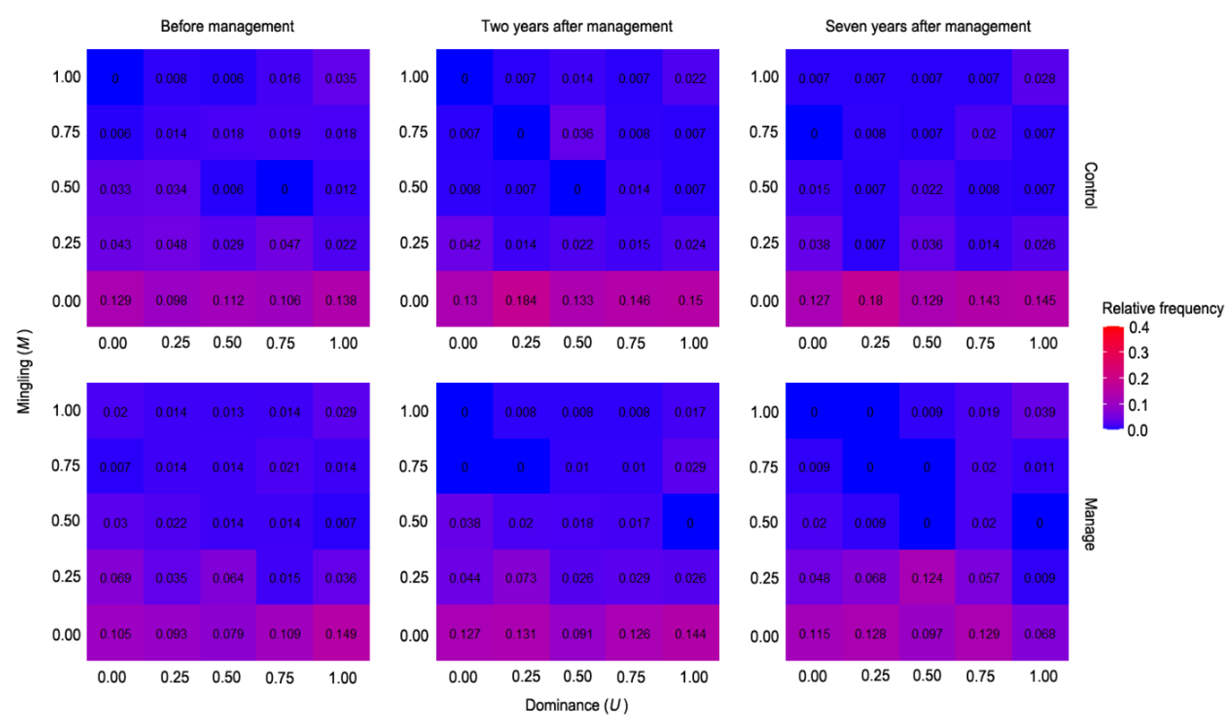
3.2.3. -
In all plots, the - bivariate distributions yielded approximately the same frequency values for each class of (0.00–1.00), whereas frequency values varied greatly among all classes (Figure 6). Most reference trees in all plots were surrounded by trees of the same species. More than 50% of trees in all plots were concentrated within the structural combination = 0.00 and = 0.00–1.00, which was evenly distributed at each level of dominance ( = 0.00–1.00). The proportion of dominant ( = 0.00, 0.25) and medium ( = 0.50) trees with a low degree of mingling ( = 0.00 and 0.25) in the SBFM plots were 0.445, 0.492, and 0.580 for management durations of 0, 2 and 7 years, respectively, whereas those in the control plots were 0.459, 0.525, and 0.517. The relative frequency of this structural combination after 7 years of management was 6.3% higher in the SBFM plots than in the control plots. The proportions of trees that had high degrees of mingling ( = 0.75, 1.00) and disadvantage ( = 1.00, 0.75) were higher in the SBFM plots (2 years, 0.064; 7 years, 0.089) than in the control plots (2 years, 0.044; 7 years, 0.062) (Figure 5).

Figure 6.
Bivariate distributions of and at different management years.
3.3. Proportions of Different Types of Random Tree
Randomly distributed trees comprised the main body of the plantation forests in this study, representing about 50% of the reference trees in all plots. Therefore, increasing the proportion of random-structure units is a main focus of plantation management. In this study, the proportion of randomly distributed trees generally increased in the SBFM plots and decreased in the control plots (Figure 3).
Regardless of the management treatment, the average frequency of R2 units (32.5–43.9%) was higher than that of R1 units (7.9–15.5%) (Table 3). As management duration increased, the average proportion of R2 units gradually decreased in the SBFM plots, whereas the average frequency of R1 units first decreased and then increased. However, the opposite trend was observed in the control plots, with the average proportion of R2 units first declining and then increasing and that of R1 units gradually declining over time (Table 3). The ratio of R2 units to R1 units shifted from 3.32 to 5.28 (average, ~4.00) (Figure 7). Thus, the frequency of R1 units in all plots was generally lower than that of R2 units. There were no significant differences in the frequencies of either R2 or R1 units or in the ratio of R2 units to R1 units between the SBFM and control plots.
Table 3.
The average frequency of R2 and R1 in total plots.
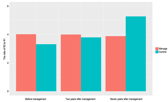
Figure 7.
The ratio of R2 to R1 between the SBFM and control plots.
4. Discussion
The goal of forest management is to improve tree competition and forest quality through structural adjustment, ultimately cultivating a healthy and stable forest [4,5,11]. Forest structure development, which is similar to the forest succession, is a long and dynamic process whose effects are not obvious within short periods of time and are difficult to predict over long periods of time (decades of recovery). Thus, it is necessary to promote the formation of a desired forest structure through effective human disturbance to accelerate the succession process and produce stable and efficient forest development. SBFM uses structural parameters to guide adjustments to optimize forest structure. It has become an effective means to guide forest structural adjustment and optimization. However, as management duration has increased, changes to stand spatial structure following SBFM have remained poorly understood. Therefore, we evaluated the effects of SBFM on the spatial structure characteristics of a P. orientalis plantation using SSSPs.
4.1. Dynamic Changes in Zero-Variate and Univariate Distributions of SSSPs
Zero-variate distributions (average value) of SSSPs, which reflect the mean state of the overall stand structure, are commonly used to statistically determine the central position of relatively concentrated data [5]. By contrast, univariate distributions of SSSPs reflect the distribution frequency of trees with specific structural features with a plot, and thus describe subtler features of stand structure [5].
is an SSSP that allows the analysis of forest spatial pattern [44]. As its mean values and frequency distributions are useful for describing the microstructure, it has been widely used to guide forest structure adjustment, simulation and reconstruction [3,15,46]. Previous studies have shown that most trees are randomly distributed ( = 0.50) in terms of quantity and basal area [47,48,49]. In this study, we found < 0.50 in all plots, which indicated that the plantation stands were in transition between a uniform and random distribution, as described in a previous study [50]. We also found that most trees in all stands were randomly distributed (W = 0.50). This result was similar to those of previous studies [47,48,49]. Furthermore, we found that the average values were higher in the SBFM plots than in the control plots, regardless of management duration, with a significant difference between the SBFM and control plots after 2 years of management (p < 0.05). This suggests that SBFM can increase the proportion of randomly distributed trees over time, as has been observed in other studies [6,26].
indicates the spatial dominance of tree species [5,51]. In our study, average values were close to 0.50 for all plots, and trees in most plots were evenly distributed at each level of dominance. These results are consistent with those of previous studies [20,50]. The implementation of SBFM slightly decreased mean dominance values over time, whereas the corresponding values of the control stands increased slightly, with significant differences between the SBFM and control plots observed throughout the 7-year management period (p < 0.05). Significant differences were also detected between 2 and 7 years of management for the combination of medium ( = 0.50) and absolutely disadvantaged ( = 1.00) trees (p < 0.05). These results suggest that SBFM can promote the growth of moderately and highly dominant trees and that their difference in dominance increases as management duration increases [6,52], This may be because SBFM adjusts the microenvironmental conditions of target trees to some extent.
Our results also showed that average values were <0.25 in all plots, which indicates suboptimal tree species diversity in the P. orientalis plantation. Species diversity is an important attribute of forests; more mingling indicates higher tree species diversity [6,20,53]. In our study, average values were higher in the SBFM plots than in the control plots, but these differences were not significant. In all plots, most trees were concentrated in the low classes (0.00, 0.25), regardless of management duration. These results indicate that the implementation of SBFM is conducive to tree growth and diversity, perhaps because the numbers of reference trees of the same species decrease during SBFM, and subsequent changes to the surrounding microenvironment promote the emergence and growth of multiple tree species. However, such changes could not be observed during this short-term study. Therefore, it is necessary to implement SBFM over a longer period to determine whether species diversity is continuously promoted under SBFM.
4.2. Dynamic Changes in Bivariate Distributions of SSSPs
Bivariate distributions of SSSPs can be used to observe two stand spatial structural features simultaneously, allowing comprehensive and accurate determination of stand spatial structure characteristics [1,6,54,55]. Previous studies have described three types of undesirable forest microstructure: disadvantaged trees with a low degree of mingling, disadvantaged trees with non-randomly distributed, and non-randomly distributed trees with a low degree of mingling. Thus, forest management strategies generally aim to decrease the proportion of trees with these microstructural characteristics. In our research, we detected significant differences between the SBFM and control plots for the structural combinations = 0.50 and = 0.50, as well as = 1.00 and = 0.50, after 2 and 7 years of management, respectively. As management duration increased, the relative frequency of trees in SBFM plots with no mixture ( = 0.00) and a random distribution ( = 0.50) decreased. Similar results were reported in a previous study [20]. In plots with a more desirable microstructure, no such significant changes were observed. We also found that the frequency of trees with a low degree of dominance ( = 0.00, 0.25) and random distribution ( = 0.50) did not differ significantly between the SBFM and control plots among management duration periods. However, the relative frequency of trees with a combination of complete mixture ( = 1.00) and random distribution ( = 0.50) gradually increased, with that in the SBFM plots higher than that in the control plots. These results suggest that SBFM can decrease the proportion of unreasonable microstructures by changing distribution pattern and mingling rates. These changes provide a scientific basis for thinning strategies [1,6,54].
4.3. Dynamic Changes in the Proportions of R1 and R2 Units
Natural forests are mainly composed of randomly distributed trees that promote forest stability [49,56]. Randomly distributed trees have greater access to light on both sides, such that a reference tree has less competitive pressure from its neighbors. In our research, the average frequency of R2 units was higher than that of R1 units, which is consistent with the findings of a previous study that reported double the proportion and basal area of R2 units compared to R1 units [49]. However, we found that the ratio of R2 to R1 changed from 3.32 to 5.28, with an average of approximately 4.00. Thus, the proportion of R2 units was about fourfold greater than that of R1 units, perhaps because of differences in the origin and succession stage of forests [56]. As management duration increased, the ratio of R2 units to R1 units gradually decreased in SBFM plots, whereas it slowly increased in the control plots. However, we detected no significant differences in the frequency of either R2 units or R1 units or in the ratio of R2 units to R1 units between the SBFM and control plots. These results indicate that SBFM can effectively adjust the ratio of R2 units to R1 units, gradually increasing the stability of plantation forests.
5. Conclusions
We studied the dynamic effects of SBFM on stand spatial structure in a P. orientalis plantation. We found that SBFM could gradually accelerate the development of the forest to a random distribution pattern, reaching a significant difference within 2 years of management. The implementation of SBFM also promoted the growth of medium and dominant trees, with a significant difference in dominance between the SBFM and control plots within 7 years of management. SBFM could slightly increase mingling compared to the control plots, although no significant differences were observed. It also decreased the proportion of undesirable microstructures in which trees were disadvantaged with a non-randomly distributed and low degree of mingling. Finally, it effectively adjusted the ratio of R2 units to R1 units, gradually improving the stability of the forest. These results demonstrate that SBFM can effectively improve the stand spatial structure in this P. orientalis plantation forest; this effect became increasingly significant as management duration increased. However, the SBFM plots still had not attained an ideal spatial structure within the 7-year management period. Therefore, SBFM should be sustained to further optimize the spatial structure of these plots. The results of this study provide basic data to guide the management of P. orientalis plantations, as well as a scientific basis for further implementation and evaluation of SBFM technology.
Author Contributions
L.Z. jointly conceived the study with G.L.; L.Z., M.D., Y.W. and J.G. designed the experiments and collected data; L.Z. and H.F. analyzed the data; L.Z. wrote the manuscript. All authors have read and agreed to the published version of the manuscript.
Funding
This research was funded by the National Science Foundation of China (Grant No. 31901309) and the Fundamental Research Funds for the Central Non-profit Research Institution of CAF (Grant No. CAFYBB2021ZK001).
Institutional Review Board Statement
Not applicable.
Informed Consent Statement
Not applicable.
Data Availability Statement
Not applicable.
Conflicts of Interest
The authors declare no conflict of interest.
References
- Zhang, L.; Hui, G.; Hu, Y.; Zhao, Z. Spatial structural characteristics of forests dominated by Pinus tabulaeformis Carr. PLoS ONE 2018, 13, e0194710. [Google Scholar] [CrossRef] [Green Version]
- Spies, T. Forest structure: A key to the ecosystem. Northwest Sci. 1998, 72, 34–39. [Google Scholar]
- Pommerening, A. Evaluating structural indices by reversing forest structural analysis. For. Ecol. Manag. 2006, 224, 266–277. [Google Scholar] [CrossRef]
- Pretzsch, H.; Zenner, E. Toward managing mixed-species stands: From parametrization to prescription. For. Ecosyst. 2017, 4, 19. [Google Scholar] [CrossRef] [Green Version]
- Hui, G.; Zhang, G.; Zhao, Z.; Yang, A. Methods of forest structure research: A review. Curr. For. Rep. 2019, 5, 142–154. [Google Scholar] [CrossRef]
- Wan, P.; Zhang, G.; Wang, H.; Zhao, Z.; Hu, Y.; Zhang, G.; Hui, G.; Liu, W. Impacts of different forest management methods on the stand spatial structure of a natural Quercus aliena var. acuteserrata forest in Xiaolongshan, China. Ecol. Inform. 2019, 50, 86–94. [Google Scholar] [CrossRef]
- Kint, V.; Meirvenne, M.; Nachtergale, L.; Geudens, G.; Lust, N. Spatial methods for quantifying forest stand structure development: A comparison between nearest-neighbor indices and variogram analysis. For. Sci. 2003, 49, 36–49. [Google Scholar]
- Enquist, B.; West, G.; Brown, J. Extensions and evaluations of a general quantitative theory of forest structure and dynamics. Proc. Natl. Acad. Sci. USA 2009, 106, 7046–7051. [Google Scholar] [CrossRef] [Green Version]
- Pommerening, A.; Meador, A. Tamm review: Tree interactions between myth and reality. For. Ecol. Manag. 2018, 424, 164–176. [Google Scholar] [CrossRef]
- Pommerening, A.; Grabarnik, P. Individual-Based Methods in Forest Ecology and Management; Springer: Cham, Switzerland, 2019. [Google Scholar]
- Gadow, K.; Zhang, C.; Wehenkel, C.; Pommerening, A.; Corral-Rivas, C.; Korol, M. Forest Structure and Diversity. In Continuous Cover Forestry; Gadow, K., Nagel, J., Saborowski, J., Eds.; Springer: Berlin/Heidelberg, Germany; Cham, Switzerland, 2012. [Google Scholar]
- Hui, G.; Zhao, X.; Zhao, Z.; Gadow, K. Evaluating tree species spatial diversity based on neighborhood relationships. For. Sci. 2011, 57, 292–300. [Google Scholar]
- Hui, G.; Wang, Y.; Zhang, G.; Zhao, Z.; Bai, C.; Liu, W. A novel approach for assessing the neighborhood competition in two different aged forests. For. Ecol. Manag. 2018, 422, 49–58. [Google Scholar] [CrossRef]
- Zhang, G.; Hui, G.; Zhang, G.; Zhao, Z.; Hu, Y. Telescope method for characterizing the spatial structure of a pine-oak mixed forest in the Xiaolong Mountains, China. Scand. J. For. Res. 2019, 34, 751–762. [Google Scholar] [CrossRef]
- Li, Y.; Hui, G.; Zhao, Z.; Hu, Y. The bivariate distribution characteristics of spatial structure in natural Korean pine broad-leaved forest. J. Veg. Sci. 2012, 23, 1180–1190. [Google Scholar] [CrossRef]
- Li, Y.; Xu, J.; Wang, H.; Nong, Y.; Sun, G.; Yu, S.; Liao, L.; Ye, S. Long-term effects of thinning and mixing on stand spatial structure: A case study of Chinese fir plantations. Iforest-Biogeo Sci. For. 2021, 14, 113–121. [Google Scholar] [CrossRef]
- Xu, J.; Zhang, G.; Zhao, Z.; Hu, Y.; Liu, W.; Yang, A.; Hui, G. Effects of randomized management on the forest distribution patterns of Larix kaempferi plantation in Xiaolongshan, Gansu Province, China. Forests 2021, 12, 981. [Google Scholar] [CrossRef]
- Dong, L.; Wei, H.; Liu, Z. Optimizing forest spatial structure with neighborhood-based indices: Four case studies from northeast China. Forests 2020, 11, 413. [Google Scholar] [CrossRef] [Green Version]
- Kang, S.; Yang, T.; Zhang, H.; Zhang, L. Dynamic visual simulation of growth and management of Chinese fir based on structured forest management. IOP Conf. Ser. Earth Environ. Sci. 2020, 502, 12038. [Google Scholar] [CrossRef]
- Fang, X.; Tan, W.; Gao, X.; Chai, Z. Close-to-nature management positively improves the spatial structure of Masson pine forest stands. Web Ecol. 2021, 21, 45–54. [Google Scholar] [CrossRef]
- Hui, G.; Gadow, K.; Hu, Y.; Xu, H. Structure-Based Forest Management; China Forestry Press: Beijing, China, 2007. [Google Scholar]
- Hui, G.; Zhao, Z.; Hu, Y. A Guide to Structure-Based Forest Management; China Forestry Press: Beijing, China, 2010. [Google Scholar]
- Hui, G.; Gadow, K. Principles of Structure-Based Forest Management; China Forestry Press: Beijing, China, 2016. [Google Scholar]
- Hui, G. Theory and Practice of Structure-Based Forest Management; Science Press: Beijing, China, 2020. [Google Scholar]
- Bettinger, P.; Tang, M. Tree-level harvest optimization for structure-based forest management based on the species mingling index. Forests 2015, 6, 1121–1144. [Google Scholar] [CrossRef]
- Wan, P.; He, R. Canopy structure and understory light characteristics of a natural Quercus aliena var. acuteserrata forest in China northwest: Influence of different forest management methods. Ecol. Eng. 2020, 153, 105901. [Google Scholar] [CrossRef]
- Dong, M.; Wang, B.; Jiang, Y.; Ding, X. Environmental controls of diurnal and seasonal variations in the stem radius of Platycladus orientalis in northern China. Forests 2019, 10, 784. [Google Scholar] [CrossRef] [Green Version]
- Du, M.; Feng, H.; Zhang, L.; Pei, S.; Wu, D.; Gao, X.; Kong, Q.; Xu, Y.; Xin, X.; Tang, X. Variations in carbon, nitrogen and phosphorus stoichiometry during a growth season within a Platycladus orientalis plantation. Pol. J. Environ. Stud. 2020, 29, 1–12. [Google Scholar] [CrossRef]
- Wang, P.; Jia, L.; Wei, S.; Wang, Q. Analysis of stand spatial structure of Platycladus orientalis recreational forest based on Voronoi diagram method. J. Beijing For. Univ. 2013, 35, 39–44. [Google Scholar]
- Zhang, L.; Sun, C.; Lai, G. Analysis and evaluation of stand spatial structure of Platycladus orientalis ecological forest in Jiulongshan of Beijing. For. Res. 2018, 31, 75–82. [Google Scholar]
- National Forestry and Grassland Administration of China. Report of Forest Resources in China (2014–2018); China Forestry Press: Beijing, China, 2019. [Google Scholar]
- Zhang, L.; Hu, Y.; Zhao, Z.; Sun, C. Spatial structure diversity of Platycladus orientalis plantation in Beijing Jiulong Mountain. Chin. J. Ecol. 2015, 34, 60–69. [Google Scholar]
- Feng, H.; Du, M.; Xin, X.; Gao, X.; Zhang, L.; Kong, Q.; Fa, L.; Wu, D. Seasonal variations in carbon, nitrogen and phosphorus stoichiometry of Platycladus orientalis plantation in the rocky mountainous areas of North China. Acta Ecol. Sin. 2019, 39, 1572–1582. [Google Scholar]
- Liu, Z.; Yu, X.; Jia, G.; Li, H.; Lu, W.; Hou, G. Response to precipitation in water sources for Platycladus orientalis in Beijing mountain area. Sci. Silvae Sin. 2018, 57, 16–23. [Google Scholar]
- Wu, B.; Zhou, L.; Qi, S.; Jin, M.; Lu, J. Effect of habitat factors on the understory plant diversity of Platycladus orientalis plantations in Beijing mountainous areas based on maxent model. Ecol. Indic. 2021, 129, 107917. [Google Scholar] [CrossRef]
- Li, W.; Zhao, X.; Bian, J.; Liu, R.; Ni, R. Regeneration characteristics and spatial pattern of Platycladus orientalis in mount Tai, China. Open J. Ecol. 2021, 11, 276–286. [Google Scholar] [CrossRef]
- Liu, J.; Ha, V.N.; Shen, Z.; Zhu, H.; Zhao, F.; Zhao, Z. Characteristics of bulk and rhizosphere soil microbial community in an ancient Platycladus orientalis forest. Appl. Soil Ecol. 2018, 132, 91–98. [Google Scholar] [CrossRef]
- Wang, P.; Xing, C.; Jia, L.; Wen, J.; Yun, X. Effect of different tending regimes on scenic quality of the Platycladus orientalis recreational forest. Sci. Silvae Sin. 2013, 49, 85–92. [Google Scholar]
- Wang, P.; Jia, L.; Li, X.; Jiang, L. Effect of tending on species composition and diversity of undergrowth in Platycladus orientalis recreational stands. J. Northeast For. Univ. 2012, 40, 78–82. [Google Scholar]
- Duan, J.; Ma, L.; Jia, L.; Jia, Z.; Gong, N.; Che, W. Effect of thinning on Platycladus orientalis plantation and the diversity of undergrowth vegetation. Acta Ecol. Sin. 2010, 30, 1431–1441. [Google Scholar]
- Hui, G.; Gadow, K.; Hu, Y. The optimum standard angle of the uniform angle index. For. Res. 2004, 17, 687–692. [Google Scholar]
- Chai, Z.; Sun, C.; Wang, D.; Liu, W.; Zhang, C. Spatial structure and dynamics of predominant populations in a virgin old-growth oak forest in the Qinling Mountains, China. Scand. J. For. Res. 2016, 32, 19–29. [Google Scholar] [CrossRef]
- Zhang, G.; Hui, G.; Yang, A.; Zhao, Z. A simple and effective approach to quantitatively characterize structural complexity. Sci. Rep. 2021, 11, 1326. [Google Scholar] [CrossRef]
- Hui, G.; Gadow, K. Das Winkelmass—Theoretische Überlegungen zum optimalen Standardwinkel. Allg. Forst Jagdztg. 2002, 173, 173–177. [Google Scholar]
- Wickham, H. ggplot2: Elegant Graphics for Data Analysis; Springer: New York, NY, USA, 2016. [Google Scholar]
- Zhao, Z.; Hui, G.; Hu, Y.; Wang, H.; Zhang, G.; Gadow, K. Testing the significance of different tree spatial distribution patterns based on the uniform angle index. Can. J. For. Res. 2014, 44, 1417–1425. [Google Scholar] [CrossRef]
- Zhang, G.; Hui, G.; Zhao, Z.; Hu, Y.; Wang, H.; Liu, W.; Zang, R. Composition of basal area in natural forests based on the uniform angle index. Ecol. Inf. 2018, 45, 1–8. [Google Scholar] [CrossRef]
- Li, Y.; He, J.; Yu, S.; Wang, H.; Ye, S. Spatial structures of different-sized tree species in a secondary forest in the early succession stage. Eur. J. For. Res. 2020, 139, 709–719. [Google Scholar] [CrossRef]
- Zhang, G.; Hui, G. Random trees are the cornerstones of natural forests. Forests 2021, 12, 1046. [Google Scholar] [CrossRef]
- Cao, X.; Li, J.; Feng, Y.; Hu, Y.; Zhang, C.; Fang, X.; Deng, C. Analysis and evaluation of the stand spatial structure of Cunninghamia lanceolata ecological forest. Sci. Silvae Sin. 2015, 51, 37–48. [Google Scholar]
- Zhao, Z.; Hui, G.; Hu, Y.; Li, Y.; Wang, H. Method and application of stand spatial advantage degree based on the neighborhood comparison. J. Beijing For. Univ. 2014, 36, 78–82. [Google Scholar]
- Aguirre, O.; Hui, G.; Gadow, K.; JimeÂnez, J. An analysis of spatial forest structure using neighborhood-based variables. For. Ecol. Manag. 2003, 183, 37–145. [Google Scholar] [CrossRef]
- Pommerening, A.; Uria-Diez, J. Do large forest trees tend towards high species mingling? Ecol. Inform. 2017, 42, 139–147. [Google Scholar] [CrossRef]
- Li, Y.; Hui, G.; Ye, S.; Hui, G.; Hu, Y.; Zhao, Z. Spatial structure of timber harvested according to structure-based forest management. For. Ecol. Manag. 2014, 322, 106–116. [Google Scholar] [CrossRef]
- Li, Y.; Li, M.; Li, X.; Liu, Z.; Ming, A.; Lan, H.; Ye, S. The abundance and structure of deadwood: A comparison of mixed and thinned Chinese fir plantations. Front. Plant Sci. 2021, 12, 614695. [Google Scholar] [CrossRef]
- Hui, G.; Zhao, Z.; Zhang, G.; Hu, Y. The role of random structural pattern based on uniform angle index in maintaining forest stability. Sci. Silvae Sin. 2021, 57, 23–30. [Google Scholar]


Publisher’s Note: MDPI stays neutral with regard to jurisdictional claims in published maps and institutional affiliations. |
© 2022 by the authors. Licensee MDPI, Basel, Switzerland. This article is an open access article distributed under the terms and conditions of the Creative Commons Attribution (CC BY) license (https://creativecommons.org/licenses/by/4.0/).