Hardwood Grain Image Restoration and Enhancement via Gaussian Histogram Specification and Adaptive Color Adjustment

Abstract

Hardwood is widely used in the surface decoration of furniture and wood products due to its rich texture and durable surface, and the improvement of wood grain images is vital to promote the aesthetics of wood surfaces. In order to restore the Gaussian distribution of distorted wood grain images and reproduce a sharp and clear wood surface, a Gaussian histogram specification algorithm based on the constant mean and variance values of red (R), green (G), and blue (B), and an adaptive color adjustment algorithm based on the color extension of R, G, and B histograms was proposed, respectively. Objective evaluation methods of histogram distribution, colorfulness index, contrast index, and sharpness index were used independently to evaluate the visual effect of the images processed by the two algorithms. Objective and subjective evaluation results showed that although the Gaussian method had only a small influence on the visual effect of hardwood grain images, it could restore the distorted images by repairing the irregular color points to weaken the adverse impact on visual impression. Meanwhile, extra attention should be paid to the processing of images with prominent uneven color transitions, because the Gaussian method might have an imperceptible smoothing or enhancing effect. The adaptive color adjustment method had a favorable enhancement effect on most hardwood grain images. However, the color extension coefficients of the over-enhanced images should be reduced to eliminate overcompensation and color shift. Compared with the traditional enhancement method unsharp mask (USM) and the methods designed for sand-degraded images and underwater images, the proposed adaptive color adjustment at the 1.5 coefficient could effectively enhance the images from the perspective of wood grain visibility and color retention.

1. Introduction

Surface decoration methods of wood products are becoming dependent on wood grain images, especially 3D wood texture printing on board surfaces [1]. A wood grain image is generally obtained through high-quality image acquisition equipment; hence it belongs to natural images (NI), whose pixel intensity follows the Gaussian distribution [2]. Because of the instability of image acquisition equipment and other factors, the image quality of wood grain is apt to degrade, and the pixel intensity of the distorted images does not always follow the Gaussian distribution. For instance, noise is typically strongest in the B (blue) channel of an image [3], and disobeys the Gaussian distribution. Therefore, when it comes to the digital printing of wood grain images, image enhancement approaches like output sharpening are essential to produce a satisfactorily clear wood surface [4]. As a result, the restoration and enhancement of wood grain images are vital to promote the aesthetics of a wood surface.

Currently, most image restoration and enhancement methods concentrate on underwater images [5,6,7], haze images [8,9], or sand-dust images [10,11] because of the poor image acquisition environment. As the vision sensor works in a low-light environment and the imaging quality is vulnerable to water, fog, and dust, image distortion such as colorfulness reduction, contrast change, degradation, noise contamination, and blur always occur. However, because the acquisition of wood grain images is normally carried out in a clean and static environment, these methods are not applicable to the wood images. Therefore, only a few studies exist which focus on the restoration and the enhancement of wood grain images [12,13].

There were also plenty of studies about image quality assessment (IQA) [14,15,16], but only a few of them reported on wood images. Rajagopal et al. [16] proposed a wood No-reference IQA (WNR-IQA) metric to assess the quality of wood images, and yet the metric was based on grayscale images. The analyses on wood images are usually performed to realize color classification, texture recognition [17], and wood species identification [18,19].

In order to restore the distorted wood grain images by approximating the Gaussian distribution of natural images (NI), a method of Gaussian histogram specification based on the constant mean and variance values of red (R), green (G), and blue (B) was proposed. Additionally, to print wood grain images and reproduce a satisfactorily clear wood surface, an adaptive color adjustment algorithm was proposed in which the histogram distributions of R, G, and B channels were extended respectively to enhance the images.

Histograms describe the quantitative characteristics and reflect the statistical distribution of the colors in an image [10]. More importantly, the restoration and enhancement effect of the corrected images can be evaluated through the distribution of the RGB histograms [7,8].

Existing color image restoration and enhancement methods are mostly based on image contrast [20] and sharpness [21]. Contrast is the difference in visual characteristics that make an object more recognizable [22]. Nordvik et al. [23] proved that contrast is the most important property when visualizing wood, both for good and bad visualization. Sharpness can be seen as the contrast of edges; it is a pivotal factor to the human impression of image definition [24]. Furthermore, it is known that color is one of the most important parameters of the aesthetic performance of wood surfaces [3].

Based on the information discussed above, histogram distribution, colorfulness index, contrast index, and sharpness index were used independently to evaluate the visual effects of wood grain images before and after the Gaussian histogram specification and the adaptive color adjustment.

2. Materials and Methods

2.1. Pretreatment of Wood Grain Images

Hardwood is widely used in the surface decoration of furniture and wood products, such as solid wood panels and wood veneer, due to its rich texture and durable surface [17]; hence we chose ten hardwood grain images with distinct colors from ten tree species on a public wood database website [25] as the experimental objects. The rich texture of hardwood can also be conducive to deepening the visual impression for better observation. The basic information of the ten species is shown in

Table 1. Basic information of the ten tree species.

Serial Numbers	Tree Name	Scientific Name	Thumbnails
1	Mun Ebony	Diospyros mun
2	Indian Silver Greywood	Terminalia bialata
3	Macassar Ebony	Diospyros celebica
4	Brazilwood	Paubrasilia echinata
5	Dogwood	Cornus florida
6	Jarrah	Eucalyptus marginata
7	Southern Magnolia	Magnolia grandiflora
8	Afata	Cordia trichotoma
9	Golden Wattle	Acacia pycnantha
10	American Elm	Ulmus americana

.

The ten hardwood images were stored in a default JPEG format at 8 bits per channel and 300 pixels per inch (ppi) resolution. They were then cropped to the size of 35 mm × 35 mm (length × width); thus, the size of each image is 413 × 413 pixels with 256 gray levels.

2.2. Gaussian Histogram Specification of Wood Grain Images

Histogram specification is a kind of typical non-modeled image intensification method [26]. Due to the fact that the I channel of HSI images is the main factor that restricts the production of crisper looking haze images, to intensify the image contrast, Liang et al. [8] proposed a color image defogging algorithm through the histogram specification of Gaussian function weighting on the I channel.

Since the R, G, and B components of RGB images were equally related to the intensity component I of HSI images, the Gaussian histogram specification was conducted on the R, G, and B channels, respectively. Different from the above intensifying method, to approximate the RGB histograms of the natural images (NI), the Gaussian method was conducted under the condition that the mean and variance values of each image were constant. The Gauss formulas are as follows:

$$f\left(x\right)=\frac{1}{\sqrt{2\pi {\sigma }_c}}\exp \left(-\frac{{\left(x-{\mu }_c\right)}^2}{2{\sigma }_c{}^2}\right)$$

(1)

$${\sigma }_c{}^2={\displaystyle \sum }_i{\displaystyle \sum }_j{\left[I_c\left(i,j\right)-{\mu }_c\right]}^2$$

(2)

$${\mu }_c=\frac{1}{MN}{\displaystyle \sum }_i{\displaystyle \sum }_j{I}_c\left(i,j\right)$$

(3)

where $c\in \left\{R,G,B\right\}$, ${\sigma }_c{}^2$ is the image variance, ${\mu }_c$ is the average value of all pixels in the image, $M\times N$ is the image size, and $I_c\left(i,j\right)$ is the pixel value at the point $\left(i,j\right)$.

2.3. Adaptive Color Adjustment of Wood Grain Images

The existing image enhancement algorithms mainly focus on the color deviation caused by the shooting environment, thus each color channel is treated differently. For example, as shown in Equation (4), Zhi et al. [27] used the histogram distribution of the G channel to calculate the color extension coefficient of all the channels in order to enhance the dust-degraded images.

$${\alpha }_G=\frac{255}{I_{\mathrm{G}\_max}-I_{\mathrm{G}\_min}}$$

(4)

where $I_{\mathrm{G}\_max}$ and $I_{\mathrm{G}\_min}$ are the maximum and minimum values in the G channel.

Accordingly, because there were no severely unbalanced color defects in the wood images, values of R, G, and B channels were all used to calculate the coefficient of the corresponding channel. The coefficient is calculated as follows:

$${\alpha }_c=\frac{255}{I_{c\_max}-I_{c\_min}}$$

(5)

where $c\in \left\{R,G,B\right\}$, $I_{c\_max}$ and $I_{c\_min}$ are the maximum and minimum values in each channel. As the maximum pixel value was 255 for 8-bit/channel images, the molecule 255 was used to ensure that the ${\alpha }_c$ was no less than 1.

The adaptive color adjustment is as shown by Equation (6). Then the wood grain images after the adjustment can be obtained.

$$\left\{\begin{array}{c}{I^{\prime }}_c\left(i,j\right)={\mu }_c-{\alpha }_c\times \left({\mu }_c-I_c\left(i,j\right)\right),I_c\left(i,j\right)\le {\mu }_c\\ {I^{\prime }}_c\left(i,j\right)={\mu }_c+{\alpha }_c\times \left(I_c\left(i,j\right)-{\mu }_c\right),I_c\left(i,j\right)>{\mu }_c\end{array}\right.$$

(6)

where $c\in \left\{R,G,B\right\}$, ${\mu }_c$ is the average value of all pixels in the image, $I_c\left(i,j\right)$ is the pixel value at the point $\left(i,j\right)$ before the extension adjustment, and ${I^{\prime }}_c\left(i,j\right)$ is that after the adjustment.

2.4. Objective Evaluation Indices

As the evaluation of visual effect is influenced by human subjective consciousness, objective evaluation is necessary to verify the restoration and enhancement methods adopted in image processing [5].

Color image quality can be objectively evaluated using different image attributes [14,28]. Panetta et al. [14] proposed a color quality enhancement (CQE) metric consisting of colorfulness, sharpness, and contrast to measure the color image quality, and summarized that the CQE method was applicable to a wider variety of distorted images.

In this study, considering the prior knowledge of the restored and enhanced images was available and there was no need for distortion-free images, the objective evaluation indices of colorfulness, sharpness, and contrast were used independently to evaluate the visual effect.

2.4.1. Colorfulness Index

Colorfulness is the degree of difference between a color and grayscale image [28]. As shown in Equation (7), the color image quality index (CIQI) colorfulness [29] was applied to measure the colorfulness of wood grain images.

$$CIQ{I}_{\_Colorfulness}=\frac{\sqrt{{\sigma }_{\alpha }{}^2+{\sigma }_{\beta }{}^2}+0.3\sqrt{{\mu }_{\alpha }{}^2+{\mu }_{\beta }{}^2}}{85.59}$$

(7)

where $\alpha =R-G$, $\beta =0.5\times \left(\mathrm{R}+\mathrm{G}\right)-\mathrm{B}$, ${\sigma }_h{}^2$ and ${\mu }_h$ represent the variance and average values of the two-color axes.

2.4.2. Contrast Index

Contrast is defined as the ability to separate image details [28]. The existing contrast measures are commonly based on root mean square (RMS) contrast, Weber contrast, and Michelson contrast [5,14]. In this study, the sum values of edge blocks in an image were applied to measure the RMS contrast of wood grain images.

According to Ferzli et al. [30], a Sobel edge detector is first run on each block to detect the edge blocks through the number of edge pixels in one block. For a 64 × 64 block, if the threshold is over 0.2% of the total number of pixels in one block, the block is seen as an edge block; otherwise, it is seen as a smooth block. Therefore, each wood image is divided into 64 × 64 blocks. As shown in Equation (8), the contrast of a color image is the sum of the RMS_{_contrast} values of all the edge blocks.

$$RMS{\_}_{Contrast}={\displaystyle \sum }_{i=1}^T\sqrt{\frac{1}{MN}{\displaystyle \sum }_{i=0}^{M-1}{\displaystyle \sum }_{j=0}^{N-1}{\left(I\left(i,j\right)-\mu \right)}^2}$$

(8)

where $\mu$ is the average value of all pixels in the image, $M\times N$ is the image size, $I\left(i,j\right)$ is the pixel value at the point $\left(i,j\right)$, and $T$ is the number of edge blocks.

2.4.3. Sharpness Index

Sharpness is the attribute related to the ability to preserve fine details and edges, and is defined by the boundaries between zones of different colors or intensities [28]. Since the Weber contrast-based measure of enhancement (EME) [31] can be applied to uniform background images [14], it was applied to measure the sharpness of wood grain images on the grayscale edge with an overlapped window size of 3 × 3. The formula is as follows:

$$EME{\_}_{Sharpness}=\frac{1}{k_1{k}_2}{{\displaystyle \sum }}_{l=1}^{k_1}{{\displaystyle \sum }}_{k=1}^{k_2}20Iog\left(\frac{I_{max,k,l}}{I_{min,k,l}}\right)$$

(9)

where the image is split into $k_1\times k_2$ blocks of sizes, $l_1\times l_2$, $I_{max,k,l}$ and $I_{min,k,l}$ are the maximum and minimum values inside a subblock.

3. Results and Discussion

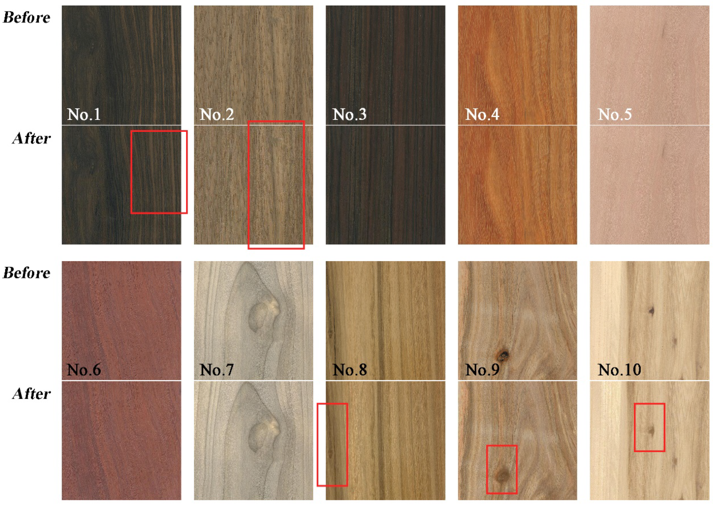
3.1. Change of Original Images after the Gaussian Histogram Specification

Figure 1 shows the visual effect of the ten hardwood grain images before and after the Gaussian histogram specification. The ${\mu }_c$ and ${\sigma }_c{}^2$ of each image remained unchanged during the process.

It can be seen from Figure 1 that there is no obvious change in the image textures after the specification except for a few marked areas.

To further find out the imperceptible change, we drew the RGB histograms of all the images and calculated the objective evaluation values before and after the specification by Equations (8)–(10). Figure 2 shows the RGB histograms of the ten images before and after the Gaussian histogram specification. The abscissa $x$ is the pixel value, and the ordinate $p\left(x\right)$ is the proportion of the normalized $x$ value. Figure 3 shows the changing trends of objective evaluation values.

From Figure 2, the RGB histograms of most images before and after the specification were almost coincident, which further implied the small influence that the Gaussian method had on the ten images. However, the marked area of the No.10 image disobeyed the Gaussian distribution. This is because when the algorithm was based on the mean and variance values, the R channel overcompensation could be easily induced [7]; even though, from Figure 1 and Figure 3, the mean and variance value-based Gaussian method had no adverse influence on visual impression of the No.10 image.

In Figure 3, the colorfulness values of the No.1, the No.8, and the No.9 images showed a wider decline after the specification. Correspondingly, in Figure 1, the textures of the No.1 image and the tree knots of the No.8 and the No.9 images were weakened. It was also found that in Figure 3, the contrast and sharpness values of the No.2 image had the largest variation after the specification. Correspondingly, in Figure 2, the RGB histograms of the No.2 image exhibited the greatest change. This phenomenon suggests that there could be a connection in each image between the histogram height and the sharpness or contrast. Moreover, the sensitivity of sharpness index was higher than the contrast index when comparing them with the RGB histograms before and after the processing.

Combined with the marked areas of these images in Figure 1, we supposed that the proposed Gaussian method tended to weaken irregular color points like tree knots, and smooth or enhance the uneven color transitions of the image textures.

To verify this conjecture, we took four grayscale images to imitate the tree knots and the edges of image textures, and then processed them by Gaussian histogram specification. Figure 4 shows the visual effect of the grayscale images and the magnified No.3 images before and after the specification. The ${\mu }_c$ and ${\sigma }_c{}^2$ of each image remained unchanged during the process.

As can be seen from Figure 4, the Gaussian method increased or decreased the difference of grayscale values between two gradients. As a result, extra attention should be paid to the processing of images with prominent uneven color transitions, because the Gaussian method might have a smoothing effect or an enhancing effect on these images.

Moreover, it made the spots fade away, and the variation of the magnified No.3 image also demonstrated this effect. It turned out that the Gaussian method could repair the irregular color points on hardwood grain images.

3.2. Change of Gaussian Images after the Adaptive Color Adjustment

Figure 5 shows the visual effect of the ten Gaussian hardwood grain images before and after the adaptive color adjustment.

As shown in Figure 5, the image contrast was increased, the brightness was improved, and the visual information was richer, but the No.3 and No.10 images seemed over enhanced and presented an unnatural look. To explore the specific variation tendency of hardwood grain images before and after the adjustment, RGB histograms, colorfulness index, contrast index, and sharpness index were used independently to evaluate the enhancement effect of the ten Gaussian images.

Similarly, we drew the RGB histograms of all the images and calculated the objective evaluation values before and after the adjustment by Equations (8)–(10). Figure 6 shows the RGB histograms of the ten Gaussian images before and after the adjustment. The abscissa $x$ is the pixel value, and the ordinate $p\left(x\right)$ is the proportion of the normalized $x$ value. Figure 7 shows the changing trends of objective evaluation values.

As seen in Figure 6, the histogram distributions of the R, G, and B channels became more dispersed and uniform after the adjustment, which was consistent with the high visual characteristics of enhanced images [7,8]. Moreover, from Figure 7, the evaluation values of colorfulness, contrast, and sharpness all increased to varying degrees.

However, it could be seen from Figure 6 that the histograms of the No.1, the No.3, the No.5, and the No.10 images after the adjustment were evidently overcompensated in the R, G and B channels, and the R channel of the No.10 image was especially obvious. The reason for this phenomenon could be the same as that caused by the Gaussian method.

3.3. Improvement and Comparison of the Adaptive Color Adjustment Algorithm

According to the Equation (6), the overcompensation in the R, G and B channels of the color-adjusted images might not only be induced by the mean value-based algorithm, but also by the color extension coefficient ${\alpha }_c$. Therefore, we compared the ${\alpha }_c$ values of all the images in

Table 2. Values of the color extension coefficient ${\alpha }_c$ of the ten Gaussian images.

Index	No.1	No.2	No.3	No.4	No.5	No.6	No.7	No.8	No.9	No.10
${\alpha }_R$	2.361	1.441	3.110	1.771	2.361	1.527	1.536	1.393	1.564	2.073
${\alpha }_G$	2.629	1.417	3.228	1.656	2.257	1.711	1.509	1.335	1.500	1.645
${\alpha }_B$	2.865	1.466	3.400	1.678	2.217	1.759	1.527	1.500	1.635	1.614

.

From Table 2, the ${\alpha }_c$ values of the No.1, the No.3, and the No.5 images were over 2, and the ${\alpha }_R$ value of the No.10 image was also over 2. Combined with the marked areas in Figure 6, it was proven that the overcompensation could also be caused by the ${\alpha }_c$ values.

For the other appropriately enhanced images, the ${\alpha }_c$ values were around 1.5. Consequently, we reset the coefficient to a unified 1.5, and then drew the RGB histograms of the color-adjusted images at this setting. Figure 8 shows the RGB histograms of the four Gaussian images before and after the adjustment.

As seen in Figure 8, though the RGB histograms were not as dispersed as those in Figure 6, the overcompensation in the R, G and B channels disappeared at the reduced ${\alpha }_c$ setting, excluding the No.10 image. This was because the No.10 image was already overcompensated during the Gaussian process.

Notably, another adjustment experiment was conducted under which the coefficient was reset to a unified 2. The overcompensation in the No.1 and the No.3 images almost disappeared, but it was still appreciable in the No.5 and No.10 images. That is, for the light-colored images, overcompensation could be more easily induced by the mean and variance value-based algorithms.

Images processed by the traditional output sharpening method unsharp mask (USM) were compared with those processed by the proposed algorithm at the unified 1.5 value of ${\alpha }_c$. When the amount was set to 50 (%), the radius 1.5 (pixels), and the threshold 0 (levels) in USM, images presented a more ideal and higher sharpness [24].

Table 3. Objective evaluation values of the four Gaussian images after the adaptive color adjustment at different ${\alpha }_c$ values and the USM sharpening.

Index	No.1			No.3			No.5			No.10
	${\alpha }_R$ = 2.4 ${\alpha }_G$ = 2.6 ${\alpha }_B$ = 2.9	${\alpha }_c$ = 1.5	USM	${\alpha }_R$ = 3.1 ${\alpha }_G$ = 3.2 ${\alpha }_B$ = 3.4	${\alpha }_c$ = 1.5	USM	${\alpha }_R$ = 2.4 ${\alpha }_G$ = 2.3 ${\alpha }_B$ = 2.2	${\alpha }_c$ = 1.5	USM	${\alpha }_R$ = 2.1 ${\alpha }_G$ = 1.6 ${\alpha }_B$ = 1.6	${\alpha }_c$ = 1.5	USM
Colorfulness	0.59	0.34	0.16	0.78	0.26	0.13	0.29	0.23	0.21	0.53	0.40	0.33
Contrast	22.99	13.78	11.63	21.14	10.73	8.85	23.27	17.39	16.16	21.95	18.77	15.36
Sharpness	18.60	9.29	7.75	16.20	5.84	4.32	3.10	0.69	0.38	0.64	0.12	0.04

shows the objective evaluation values of the four images processed by the proposed algorithm whose ${\alpha }_c$ values were from Table 2 and a unified 1.5, and by the USM at the mentioned setting.

As shown in Table 3, a higher ${\alpha }_c$ value represents a higher evaluation value of the three indices, and a higher possibility of resulting in overcompensation. The visual effect of the No.10 image enhanced by the above methods is shown below.

From Figure 9, the ${\alpha }_c$ values obtained by Equation (5) were not appropriate for the adaptive color adjustment of the No.10 image, as its color was quite different from that of the original image, inclined to green. On the contrary, the algorithm at the reduced ${\alpha }_c$ values (a unified 1.5) not only effectively enhanced the images, but also performed better in the enhancement effect than the USM. Despite the No.10 image still displayed overcompensation after the color adjustment at the reduced coefficient, the negative impact on visual impression was alleviated.

To further verify the effectiveness and the applicability of the proposed algorithm in other wood grain images, we performed qualitative and quantitative comparisons with the following methods: the adaptive color adjustment algorithm proposed by Zhi et al. [27] for sand-degraded images, the color balance algorithm proposed by Luo et al. [5] for underwater images, the traditional enhancement method USM suggested by Mao et al. [24], and the proposed adaptive color adjustment algorithm for wood grain images before and after modification.

The tested images were from another five tree species, and stored in the same format and size as described above after being processed by the Gaussian histogram specification. Then, these Gaussian images were processed by the adjusted methods discussed above, respectively, and the resulting visual effect is shown in Figure 10. The basic information of the five species is shown in

Table 4. Basic information of the five tree species.

Serial Numbers	Tree Name	Scientific Name	Thumbnails
11	Balsa	Ochroma pyramidale
12	Itin	Prosopis kuntzei
13	Crab Apple	Malus domestica
14	Butternut	Juglans cinerea
15	Water Hickory	Carya aquatica

.

Clearly, from the perspective of image enhancement and color adjustment, the algorithms designed for sand-degraded images and underwater images were not suitable for wood grain images, and the USM was also unsatisfactory in improving image grain visibility. The proposed algorithm was better than these methods in improving visibility and maintaining color, but some of the images were over enhanced, especially the light-colored images, leading to overcompensation and color shift. Consequently, the color extension coefficient of the proposed algorithm should be reduced.

Thanks to the high similarity between the images processed by the USM and the Propose-2 in Figure 10, further comparison was made through the objective evaluation below.

As can be seen from

Table 5. Objective evaluation values of the five Gaussian images after the USM sharpening and the adaptive color adjustment.

Index		No.11	No.12	No.13	No.14	No.15
Colorfulness	O 1	0.165	0.226	0.228	0.236	0.467
	G + USM 2	0.156	0.187	0.230	0.227	0.462
	G + H 3	0.211	0.316	0.267	0.306	0.666
Contrast	O	8.381	8.672	5.567	14.237	15.676
	G+USM	10.675	10.876	6.617	18.331	20.914
	G+H	11.773	12.536	7.712	21.556	22.840
Sharpness	O	0.000	0.942	0.000	0.093	0.254
	G+USM	0.000	2.599	0.000	0.182	0.516
	G+H	0.000	3.489	0.001	0.328	0.618

¹ O represents original images; ² G + USM represents images processed by the Gaussian method and the USM; ³ G+H represents images processed by the Gaussian method and the histogram extension method at the unified 1.5 coefficient.

, the five Gaussian images processed by the histogram extension method at the unified 1.5 coefficient performed better than USM in colorfulness, contrast, and sharpness, which verified the effectiveness of our algorithm. Despite the fact that the sharpness value of the No.11 image could not be calculated because of its inapparent texture, the results of other images remained effective.

4. Conclusions

In order to restore the distorted wood grain images by approximating the Gaussian distribution of natural images (NI), a method of Gaussian histogram specification was proposed. In addition, to print digital wood grain and reproduce a satisfactorily clear wood surface, an adaptive color adjustment algorithm was proposed and improved. Good processing results were achieved by using the proposed algorithms.

The Gaussian histogram specification was based on the constant mean and variance values of the R, G, and B of each image. The changing trends of the RGB histograms, colorfulness index, contrast index, and sharpness index of each image varied after the specification. Though the Gaussian method had a small influence on the visual effect of hardwood grain images, it could restore the distorted images by repairing the irregular color points to weaken the adverse impact on visual impression. The Gaussian method also had a smoothing effect or an enhancing effect on the images with prominent uneven color transitions.

The adaptive color adjustment was based on the color extension of the R, G, and B histograms of each Gaussian image. The texture visibility was improved, and the details were highlighted for each Gaussian image after the adjustment. The evaluation indices of colorfulness, contrast, and sharpness all showed an upward trend, and the distribution of the RGB histograms became more dispersed and uniform, implying that all the Gaussian images were enhanced after the adjustment.

Nevertheless, some of the color-adjusted images had overcompensation in R, G and B channels, which even led to color shift. By reducing the values of the color extension coefficient, the overcompensation and color shift could be eliminated. A higher coefficient represented a more scattered distribution of RGB histograms, a higher evaluation value of the three indices, and a higher enhancement intensity, yet the enhancement effect might not be satisfactory.

The adaptive color adjustment algorithm was compared with the traditional enhancement method USM and the methods designed for sand-degraded images and underwater images. The results show that images processed by the proposed algorithm at the reduced coefficient got better results in both objective and subjective evaluation, which verified the effectiveness and applicability of our algorithm in wood grain images.

From the view of digital image, the macroscopic appearance of wood grain is a region with different local color values and overall color. Although the tested images from 15 tree species could not represent the color of all the wood grain images, the color extension coefficient around 1.5 was proven to be effective. Overall, multiple tests and comparisons were suggested for different color images to obtain the required effect.

References

1. Sang, R.; Manley, A.; Wu, Z.; Feng, X. Digital 3D Wood Texture: UV-Curable Inkjet Printing on Board Surface. Coatings 2020, 10, 1144. [Google Scholar] [CrossRef]
2. Xu, M.; Li, T.; Ping, X. A New Model of Nature Images Based on Generalized Gaussian Distribution. In Proceedings of the 2009 International Conference on Communications & Mobile Computing, Washington, DC, USA, 6–8 January 2009; pp. 446–450. [Google Scholar]
3. Mao, J.; Wu, Z.; Feng, X. A Modeling Approach on the Correction Model of the Chromatic Aberration of Scanned Wood Grain Images. Coatings 2022, 12, 79. [Google Scholar] [CrossRef]
4. Fraser, B.; Schewe, J. Chapter Two: Why do we sharpen? In Real World Image Sharpening with Adobe Photoshop, Camera Raw, and Lightroom; Fraser, B., Schewe, J., Eds.; Peachpit Press: Berkeley, CA, USA, 2010; pp. 121–292. [Google Scholar]
5. Luo, W.; Duan, S.; Zheng, J. Underwater image restoration and enhancement based on a fusion algorithm with color balance, contrast optimization and histogram stretching. IEEE Access 2021, 9, 31792–31804. [Google Scholar] [CrossRef]
6. Yang, M.; Sowmya, A. An Underwater Color Image Quality Evaluation Metric. IEEE Trans. Image Process. 2015, 24, 6062–6071. [Google Scholar] [CrossRef] [PubMed]
7. Zhang, W.; Dong, L.; Zhang, T.; Xu, W. Enhancing underwater image via color correction and Bi-interval contrast enhancement. Signal Process. Image Commun. 2021, 90, 116030. [Google Scholar] [CrossRef]
8. Liang, Y.; Zhao, K.; Li, L.; Hu, J. Defogging algorithm of color images based on Gaussian function weighted histogram specification. In Proceedings of the 2016 10th International Conference on Software, Knowledge, Information Management & Applications (SKIMA), Chengdu, China, 15–17 December 2016; pp. 364–369. [Google Scholar]
9. Pan, X.; Xie, F.; Jiang, Z.; Yin, J. Haze Removal for a Single Remote Sensing Image Based on Deformed Haze Imaging Model. IEEE Signal Process. Lett. 2015, 22, 1806–1810. [Google Scholar] [CrossRef]
10. Park, T.H.; Eom, I.K. Sand-Dust Image Enhancement Using Successive Color Balance with Coincident Chromatic Histogram. IEEE Access 2021, 9, 19749–19760. [Google Scholar] [CrossRef]
11. Shi, Z.; Feng, Y.; Zhao, M.; Zhang, E. Let You See in Sand Dust Weather: A Method Based on Halo-Reduced Dark Channel Prior Dehazing for Sand-Dust Image Enhancement. IEEE Access 2019, 7, 116722–116733. [Google Scholar] [CrossRef]
12. Abdul Hamid, L.B.; Rosli, N.R.; Mohd Khairuddin, A.S.; Mokhtar, N.; Yusof, R. Denoising module for wood texture images. Wood Sci. Technol. 2018, 52, 1539–1554. [Google Scholar] [CrossRef]
13. Abdul Hamid, L.B.; Mohd Khairuddin, A.S.; Khairuddin, U.; Ruthfalydia, N.; Mokhtar, N. Texture image classification using improved image enhancement and adaptive SVM. Signal Image Video Process. 2022, 1–8. [Google Scholar] [CrossRef]
14. Panetta, K.; Chen, G.; Agaian, S. No reference color image contrast and quality measures. IEEE Trans. Consum. Electron. 2013, 59, 643–651. [Google Scholar] [CrossRef]
15. Kamble, V.; Bhurchandi, K.M. No-reference image quality assessment algorithms: A survey. Optik 2015, 126, 1090–1097. [Google Scholar] [CrossRef]
16. Rajagopal, H.; Mokhtar, N.; Tengku Mohmed Noor Izam, T.F.; Wan Ahmad, W.K. No-reference quality assessment for image-based assessment of economically important tropical woods. PLoS ONE 2020, 15, e0233320. [Google Scholar] [CrossRef] [PubMed]
17. Wang, Z.; Zhuang, Z.; Liu, Y.; Ding, F.; Tang, M. Color Classification and Texture Recognition System of Solid Wood Panels. Forests 2021, 12, 1154. [Google Scholar] [CrossRef]
18. Gurau, L.; Timar, M.C.; Porojan, M.; Ioras, F. Image processing method as a supporting tool for wood species identification. Wood Fiber Sci. 2013, 45, 303–313. [Google Scholar]
19. Rajagopal, H.; Mohd Khairuddin, A.S.; Mokhtar, N.; Ahmad, A.; Yusof, R. Application of image quality assessment module to motion-blurred wood images for wood species identification system. Wood Sci. Technol. 2019, 53, 967–981. [Google Scholar] [CrossRef]
20. Gao, C.; Panetta, K.; Agaian, S. A new color contrast enhancement algorithm for robotic applications. In Proceedings of the 2012 IEEE International Conference on Technologies for Practical Robot Applications (TePRA), Woburn, MA, USA, 23–24 April 2012; pp. 1–4. [Google Scholar]
21. Li, Y.; Lin, Y. Image sharpness evaluation based on visual importance. In Proceedings of the International Congress on Image & Signal Processing, Datong, China, 15–17 October 2016; pp. 776–780. [Google Scholar]
22. Shokrollahi, A.; Maybodi, B.; Mahmoudi-Aznaveh, A. Histogram modification based enhancement along with contrast-changed image quality assessment. Multimed. Tools Appl. 2020, 79, 19193–19214. [Google Scholar] [CrossRef]
23. Nordvik, E.; Broman, N.O. Comparison of visual properties in digital wood images. For. Prod. J. 2007, 57, 97–102. [Google Scholar]
24. Mao, J.; Wu, Z.; Feng, X. Image Definition Evaluations on Denoised and Sharpened Wood Grain Images. Coatings 2021, 11, 976. [Google Scholar] [CrossRef]
25. Meier, E. The Wood Database. 2007. (Cited 16 August 2018). Available online: https://www.wood-database.com/ (accessed on 28 February 2022).
26. Ueda, Y.; Moriyama, D.; Koga, T.; Suetake, N. Histogram Specification-Based Image Enhancement for Backlit Image. In Proceedings of the 2020 IEEE International Conference on Image Processing (ICIP), Abu Dhabi, United Arab Emirates, 25–28 October 2020; pp. 958–962. [Google Scholar]
27. Zhi, N.; Mao, S.; Li, M. Visibility restoration algorithm of dust-degraded images. J. Image Graph. 2016, 21, 1585–1592. [Google Scholar]
28. Chen, G.; Panetta, K.; Agaian, S. Color image attribute and quality measurements. Proc. SPIE Int. Soc. Opt. Eng. 2014, 9120, 91200T. [Google Scholar]
29. Hasler, D.; Susstrunk, S. Measuring colorfulness in natural images. Hum. Vis. Electron. Imaging 2003, 5007, 87–95. [Google Scholar]
30. Ferzli, R.; Karam, L.J. A no-reference objective image sharpness metric based on the notion of just noticeable blur (JNB). IEEE Trans. Image Process. 2009, 18, 717–728. [Google Scholar] [CrossRef] [PubMed]
31. Agaian, S.S.; Lentz, K.P.; Grigoryan, A.M. A New Measure of Image Enhancement. In Proceedings of the IASTED International Conference on Signal Processing & Communication, Malaga, Spain, 19–22 September 2000; pp. 19–22. [Google Scholar]
Figure 1. Ten hardwood grain images before and after the Gaussian histogram specification.
Forests 13 00863 g001
Figure 2. RGB histograms of the ten images before and after the Gaussian histogram specification.
Forests 13 00863 g002
Figure 3. Changing trends of objective evaluation values of colorfulness, contrast, and sharpness on the ten images before and after the Gaussian histogram specification.
Forests 13 00863 g003
Figure 4. Grayscale images (a) before the Gaussian histogram specification; (b) after the Gaussian histogram specification. The numbers represent the grayscale values. (c) The No.3 images before and after the Gaussian histogram specification.
Forests 13 00863 g004
Figure 5. Ten Gaussian hardwood grain images before and after the adaptive color adjustment.
Forests 13 00863 g005
Figure 6. RGB histograms of the ten Gaussian images before and after the adaptive color adjustment.
Forests 13 00863 g006
Figure 7. Changing trends of objective evaluation values of colorfulness, contrast, and sharpness on the ten Gaussian images before and after the adaptive color adjustment.
Forests 13 00863 g007
Figure 8. RGB histograms of the No.1, the No.3, the No.5, and the No.10 Gaussian images before and after the adaptive color adjustment at the unified 1.5 value of α c .
Forests 13 00863 g008
Figure 9. The No.10 images processed by (a) the Gaussian histogram specification; (b) the Gaussian method and the histogram extension method whose α c values were obtained by Equation (5); (c) the Gaussian method and the histogram extension method whose α c values were from a unified 1.5; (d) the USM at the 50 (%), 1.5 (pixels), and 0 (levels) setting.
Forests 13 00863 g009
Figure 10. Subjective comparisons on the five wood grain images. From left to right: Gaussian images, the results of Zhi et al. [27], Luo et al. [5], USM [24], the proposed algorithm before modification, and the proposed algorithm at the unified 1.5 coefficient.
Forests 13 00863 g010