Abstract
Connectivity is a landscape property that promotes gene flow between organisms located in different patches of habitat and provides a way to reduce habitat loss by maintaining flux of organisms through the landscape; it is an important factor for conservation decisions. In this study, we evaluated the structural and functional connectivity among 510 oak forest remnants in a basin in central Mexico by modeling the potential distribution of seven oak species that inhabit in it. The structural and functional connectivity of oak forest remnants was estimated by graph theory. Distribution models for all the oak species had a good level of predictability, showing that 53.16% of the basin is suitable for oaks. The importance for connectivity varied between the remnant forests. Large forest fragments had the highest values of connectivity, and small forest fragments acted as steppingstones favoring the movement of organisms among fragments. In the southern region of the basin, connected remnant forests had conformed to a large network, but in the northern region, the remnant forests were mostly isolated. Conservation of oak forests in this basin requires protection for remaining patches by preserving both large and small ones and restoring biological corridors to reduce the isolation of forest fragments.
1. Introduction
Deforestation and habitat fragmentation rates have increased in recent decades in North America, degrading soils and reducing ecosystem services [1,2,3,4,5,6]. Overall, deforestation is caused by direct factors such as the expansion of agriculture and urban areas [5,6]. The change in vegetation cover results in a fragmented landscape composed of forest remnants with different sizes and shapes that still sustain some ecological processes and values [7,8,9,10]. In other words, during fragmentation the landscape is transformed from a continuum habitat to an ensemble of fragments immersed in a matrix that is different to that of the original vegetation [8,11,12]. Given the accelerated rate of ecosystems losses, designing and implementing management strategies to conserve the remnant forest fragments and increase both the size of forest fragments and their connectivity with biological corridors is crucial.
Connectivity between isolated forest fragments is an attribute of the landscape that promotes or limits the movement of organisms [13]. Connectivity depends on the position, size and arrangement of the patches (structural connectivity) and by the movement response of organisms, such as seed dispersers, to the matrix of patches (functional connectivity) [14,15,16,17]. The analysis of connectivity identifies the degree of accessibility the organisms have to different patches in the landscape. The degree and magnitude of connectivity between forest fragments is determined by the spatial configuration of forests fragments and functional factors that promote the flux, such as the capacity of organism movement and pollen or seed dispersion between patches [14,15,16,17,18]. Particularly, functional factors are crucial to sustain genetic diversity and biodiversity, to facilitate recolonization of habitats and to reduce the risk of extinction for local species [14,17,18,19]. Overall, connectivity has been considered as a conservation strategy to alleviate the local effects of fragmentation and to facilitate the adaptability of species to perturbation and climate change [15,20].
Graph theory is a mathematical approach used to identify a network of fragments and its connectivity [21,22,23,24]. The use of this theory stems from computer science, and can incorporate species interactions and plant functional groups, among other ecological attributes [25,26,27]. It produces a graph (in our case represented by the landscape) composed of a group of nodes (habitat patches) that are connected to some degree; these connections are known as edges [22,23]. The edges between the nodes indicates ecological movement (e.g., by dispersers) that happen between them [24]. A path is a unique route that goes through a sequence of nodes. Therefore, the graph is connected if a path makes every node reachable from some other node [24]. Moreover, graphs can be composed by a set of components or subgraphs, each one defined by a group of adjacent nodes. Connections between subgraphs can be sustained by key nodes; once removed the graph would be composed of disconnected subgraphs. Under graph theory assumptions, the number of subgraphs in a highly fragmented landscape would increase and the connectivity between them would depend on key fragments, size and vicinity of the fragments and the dispersion capacity of organisms [22,23,24]. With graph theory we can evaluate the structural and functional connectivity of the landscape [14,22,23]. Therefore, this analysis it is a useful tool to guide conservation priorities and management strategies in fragmented areas [17,20,24].
Temperate forests are one of the ecosystems most impacted by human activities, and the region of North America has the highest degree of transformation from primary to secondary forests [1,2,3,4,5]. In Mexico, 219,090 km2 of temperate forests were lost in a period of 18 years (1999–2011), which represents a rate of 11,669.6 km2/year [3]. Oak forests are the most widely distributed vegetation type in temperate regions of the country [28,29,30]. In Mexico oaks radiated into ca. 160 species, of which more than half are endemic [28,31,32]. Oak forests are ecologically relevant for regulating nutrient and water cycles, storing large amounts of carbon [33,34] and providing important ecosystem services for humans [33,34,35,36]. In addition, these forests represent a transitional ecosystem between tropical or arid zones with the highland forests [37]. Historically, oaks represent a valuable resource for humans for its charcoal production and consumption exerting a constant pressure to its populations [38,39,40]. Oak forest in Mexico had an original extension of 16 million ha, of which only 10 million ha of primary forests are left; the remaining hectares are considered secondary forests [41]. As a result, the landscape is a mosaic of disturbed habitats, secondary forests, and primary forests patches [42,43]. Particularly, it has been observed that primary oak forest patches still sustain high levels of plant biodiversity that change with fragment size [44]. In addition, oak remnants have a more suitable microclimatic conditions (higher soil moisture content and lower temperature) for seedling survival than open habitats [42,45]. Moreover, oak patches offer a habitat for native felids and insects [46,47]. The center and southeast of Mexico has experienced the highest deforestation rate, and regionally, Michoacán state (central Mexico) has registered the highest deforestation rate, with 11, 156 ha lost between 2007 and 2014 [17,48,49]. In the Cuitzeo Lake Basin in Michoacán state, temperate ecosystems are constantly threatened by agriculture and avocado orchards, charcoal production and urban settlements, generating a matrix of remnants of forests [50,51,52]. In this study, we aim to characterize and evaluate the degree of structural and functional connectivity of oak (Quercus L.) forest fragments in the Cuitzeo Lake Basin (CLB) in central Mexico; in this area we can find an important number of oak species, and oak forests offer an ecological pathway between the pine ecosystem to the subtropical shrublands [38,43]. In particular, we modeled the potential distribution of seven oak species based on presence data gathered from the oak forest remnants in the basin. Then, we quantified the potential area of oak forests and their degree of connectivity. This study contributes with a fundamental tool to guide oak forest conservation and restoration efforts for fragments of all sizes and different spatial arrangements.
2. Materials and Methods
2.1. Study Site
The Cuitzeo Lake Basin is located in the Trans-Mexican Volcanic Belt between the states of Michoacán and Guanajuato (19°30′ to 20°05′ N; 100°35′ to 101°30′ W) (Figure 1) [53]. The basin has an area of ca. 4000 km2 and an altitudinal gradient from 1700 to 3420 m [54,55]. It is an endorreic basin, and all the water drains to Cuitzeo Lake, which is the second largest in Mexico [56]. The weather transitions from semiwarm subhumid conditions in the northern part to temperate subhumid conditions in the southern part of the basin [55,57]. In the basin we can find oak and pine-oak forests, sub-tropical shrublands, grassland and agriculture fields [43,58], although oak forests are the most abundant vegetation type in the basin, occupying an area of 980.3 km2 in which 16 oak species have been registered [56,58]. Particularly, in rural areas oaks are an important resource for charcoal production, which is made by traditional techniques [38,39,59]. Quercus castanea Née and Quercus laeta Liebm, which are endemic to México, are frequently used for charcoal production [38]. The management of oak species for traditional charcoal production in the basin is representative for the whole country and for other regions in the world [38,39,40,59,60,61,62,63,64,65].
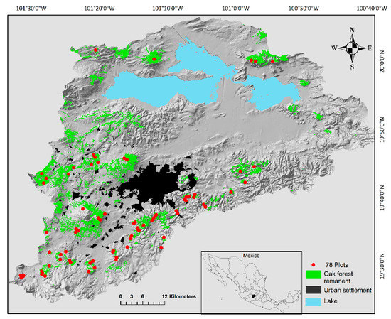
Figure 1.
The Cuitzeo lake basin in Michoacán, Mexico. In the map, oak forest remnants are indicated in green and the locations of 78 plots (census units) in red dots. The location of each unit was defined by the presence of oak forests. In each plot we registered each tree of oak species in a 2000 m2 area [43]. The oak forests remanent were identified by analyzing the 2008 vegetation layer [66,67].
2.2. Modeling the Potential Distribution of Oak Forests
To model the potential distribution of the seven most abundant oak species, we used occurrence data from censuses performed in 78 oak forest fragments in the basin between 2008 and 2009 [43]. During the censuses, in a 2000 m2 plot for each tree we recorded the diameter at breast height (dbh) and the taxonomic identity, and then estimated the species abundance, occurrence and absence record per plot (Table 1). In addition, to characterize the environmental niche of each species, with the georeferenced occurrence record we quantified bioclimatic variables (see below) from high-resolution (30 m) climatic layers by using ArcGIS ver 10.5 [68,69,70].

Table 1.
Number of occurrence records, abundance and number of absences of the seven most abundant Quercus species registered in the 78 vegetation censuses in the Cuitzeo Lake basin, Michoacán state, Mexico [43].
To identify the bioclimatic variables that explained the greatest percentage of variation and to reduce autocorrelation, we firstly performed a Principal Component Analysis (PCA) for each species to detect associations between pairs of variables [71,72,73]. Then, we explored the degree of correlation between them with a Pearson correlation analysis, and if a coefficient of correlation was >0.90 [73,74], we included only the variables that were more influential to plant performance [75]. Thus, only eight bioclimatic variables were used to model the species potential distribution (Bio3: isothermality; Bio5: maximum temperature of warmest month; Bio6: minimum temperature of the coldest month; Bio12: annual precipitation; Bio13: precipitation of the wettest month; Bio15: precipitation seasonality; Bio17: precipitation of the driest quarter; Bio18: precipitation of the warmest quarter) [68,69,70]. Then, we randomly assigned 80% of occurrence records as training data sets and the rest as testing data [76,77,78]. The species niche was modeled trough the maximum entropy model as implemented in MaxEnt. The algorithm predicts the distribution of maximum entropy for a species in an area based on climate data from where the species occurs [78]. The model contemplates that the values of climate data calculated from the predicted distribution will coincide with actual data obtained from the area of the species habit [78]. We ran the model with the predetermined parameters of the program to increase its predictive power, a maximum of 1000 iterations, a convergence limit of 0.00001 and a regularization value of 1 [78,79]. Then, we created a binary map of probability from MaxEnt, considering the maximum and minimum probability predicted by the model for each pixel that has a confirmed occurrence. The validation of the models was performed with 20% of the occurrence records assigned as testing data and with a random selection of 20% of confirmed-absences records. The models were validated through the Kappa index (K), which evaluates model accuracy based on confirmed presences and absences records from field surveys [80] and the area under the curve (AUC) value following Wollan et al. 2008 and Maya-García et al. 2020 [81,82]. The K index evaluates how many presence and absence records fell within the distribution model (suitable area) and outside (unsuitable area), it varies from 0 to 1, a high value indicates a good agreement between predictions and records [83]. For each species we retained the model with highest K index value and with values of AUC ≥ 0.9 indicating excellent model performance [81]. Finally, for each species we performed a Jacknife test in MaxEnt to identify the bioclimatic variables that had the highest influence on the AUC model.
Alternatively, to test if the models of potential distribution were also related with structural measurements of the species, we explored the relationship between the probability of occurrence of each species in the plot and the diameter at breast height and abundance through Pearson correlation analysis with R software ver. 3.5 [84,85,86].
2.3. Oak Forest Connectivity
The map of the potential distribution models with the highest K index for each oak species were used to identify the suitable area. The models of each species were intercepted with the reclassified 2008 vegetation layer (1:400,000) [66,67] with the GIS ArcMap [87,88]. The configuration of the vegetation in the landscape has not changed substantially since data were gathered [89]. We extracted all the patches within the potential distribution area of each species. We merged the maps of all the species to generate a single map with all the potential patches of oak forests in the basin.
The overall connectivity was analyzed with two dispersal (d) ranges belonging to the most important acorn disperses; a mouse species (Peromyscus melanorphrys Coues, 1874) d = 883 m and two bird species: woodpecker and charas (Melanerpes formicivorus Swainson 1827 and Aphelocoma ultramarina Bonaparte 1825, respectively) d = 10,000 [90,91,92,93,94,95]. However, in the results we emphasized the findings of the two bird species because they have an intermediate dispersal range. It has been stated that species with intermediate dispersion distance are the less sensitive to habitat loss; therefore, they are considered to be good predictors of connectivity [96]. The degree of connectivity between all the oak forest patches was evaluated with the index of the general connectivity (PC) by using Conefor Sensinode 2.2 [97].
The PC index evaluates the degree of connectivity for the landscape, including intrinsic attributes of each unit, such as patch area, habitat quality and also the topological relationships among the elements of the connectivity network (e.g., position in the landscape) [98]. The index is defined as the probability that two animals (or other species) randomly placed in the landscape fall in habitats (patches) that are interconnected based on a set of n patches and the dispersal probability (pij) among them [96]:
where ai and aj are attributes of patches i and j; in this study, we used the area of the patch as an attribute and is the total landscape area (study area). Here is the maximum product probability of all possible routes between i and j. If patches i and j are close enough it would require only one direct movement (one step) between them, which represents the maximum probability ( = pij). If there is more distance between them and more movements are required to finally connect them, the maximum probability is defined by the number of steps involved ( > pij) [96]. Our estimation of the pij was based on a negative exponential function of the Euclidean distance between nodes [24,98]. The PC index has values from 0 to 1, increasing with the degree of connectivity [96,98].
To evaluate the individual contribution of each patch to the general connectivity, we systematically removed each of the patches and then recalculated the PC index. The systematic removal of patches indicates the loss of connectivity (dPCk) and explains the importance of each patch to the connectivity [96,98]:
where PC is the connectivity index calculated for all the patches and PCremove,k is the value for the PC index without the k patch [96].
We quantified the relative value for the three components that integrate the probability of connectivity index (PC) [96]:
Habitat patches can play different functions within the landscape and the network of connectivity and the three relative fractions of the dPCk describes the different ways the k patch contributes to the connectivity [15]. The components are influenced by the area between patches, the dispersal distance of the focal species, the area of the patch and the topological position of the patch [15]. The dPCintrak is the contribution to the availability of habitat (area) of the patch k (intrapatch connectivity) [15]. This fraction is independent of the topological position of k, the intensity of connections, the dispersal capacity of species and it would have the same value even if k is completely isolated [15]. The dPCfluxk is the dispersal flux, weighted by the patch area, received or originated through links of the patch k with the rest of the patches from the landscape. This fraction is dependent on the patch k area and the topological position with respect to other patches (interpatch connectivity) and overall is an indicator of the level of connectivity of k [15,96,99]. The dPCconnectork is the function of patch k as a connector element (steppingstone) between the rest of the patches in the landscape [15]. This fraction measures the capacity of k to facilitate dispersal fluxes that are potentiated if they pass through k. This fraction is independent of the patch k area but dependent on its topological position with respect to the other patches [15,96,99]. To determine the relative contribution to the connectivity of each of the fractions (θdPCintrak, θdPCfluxk and θdPCconnectork) to the general connectivity, the sum of the dPCk was divided by the sum of each of the fractions and multiplied by 100 [15,96,98,99]. Finally, we grouped the range of values in five categories (very high, high, medium, low and very low) based on the Jenks optimization model performed in the GIS ArcMap.
3. Results
3.1. Potential Distribution of Oak Forests
For each species we retained the model of distribution with the largest value of Kappa index and AUC, indicating a higher agreement with actual presence and confirmed absence records (Table 2). Particularly, the validation of the models of distribution of each species showed Kappa values between 0.5 and 0.82, which indicates that the predictability of the models was moderate to substantial according to Landis and Koch (1977) [100] Overall, the optimum area for the distribution of oak species was ca. 212,670 ha, which represents 53.16% of the total area of the Cuitzeo Lake Basin. The potential distribution area was different for each of the seven oak species; three species had the largest distribution area, Q. castanea Née (131,235 ha), Q. deserticola Trel. (112,626 ha) and Q. laeta Liebm. (112,857 ha) (Table 2). In contrast, Q. magnoliifolia Née with 23,756 ha had the lowest area and Q. calophylla Schltdl. & Cham. was restricted exclusively to the mountain peaks (<2600 m in elevation) in the basin. (Table 2). According to Jackknife test we detected that the distribution of each species was influenced by different bioclimatic variables (Table 2). For instance, the distribution of Q. rugosa Née was determined by the minimum temperature of the coldest month (Bio6) and for Q. magnoliifolia and Q. deserticola it was affected by annual precipitation (Bio12) and by precipitation of the driest quarter (Bio17). Finally, we detected a significant correlation between the probability of distribution and a structural measurement only for Q. calophylla (probability of occurrence vs. dbh: r = 0.82, p = 0.008).
Table 2.
Potential distribution area (ha) for the models with the highest Kappa index and Area Under the Curve (AUC) and the most influential bioclimatic variables to the distribution explored through a Jackknife test of the seven most abundant oak species in the Cuitzeo Lake Basin, Michoacán, Mexico. Acronyms: Bio3: isothermality; Bio6: minimum temperature of the coldest month; Bio12: annual precipitation; Bio13: precipitation of the wettest month; Bio15: precipitation seasonality; Bio17: precipitation of the driest quarter; Bio18: precipitation of the warmest quarter.
3.2. Oak Forests Connectivity and Conservation Priorities
After intercepting the merged map of potential distribution of all the species with the 2008 vegetation layer, we obtained 510 oak forests patches, the mean area was 142.6 ha, but the area ranges from 0.2 to 10,872 ha. Furthermore, only 16 patches had an area bigger than 1000 ha and 95% of the patches had an area smaller than 500 ha (Figure 2). Therefore, given its low abundance actions need to be implemented to avoid further fragmentation of the bigger size patches. Overall, mean distance between patches was 34.6 km, the minimum distance (1.1 km) was registered between two patches located in the east portion of the basin. In contrast, the largest distance was detected between the northernmost patch and the southernmost patch (99.8 km) (Figure 2). The probability index of general connectivity (PC) calculated with the dispersal distance of 10,000 m was very low (0.023) and it was even further lower for the distance of the mice species (PC = 0.006) that has a more limited mobility (883 m). In general, the patch connectivity changed regionally (Figure 3). At the north part of the basin, we detected five subgroups of patches, and three isolated patches (Figure 3) with no apparent connection between them. We also detected that component 3 was isolated in the middle of the basin. The landscape changes from the east, south and west part of the basin, where all patches conformed to a large component (Figure 3).
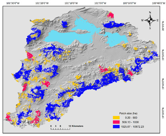
Figure 2.
Size (ha) of oak forest fragments in the Cuitzeo Lake Basin. Size categories are shown in the figure.
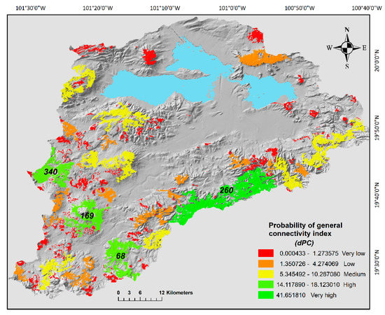
Figure 3.
Probability of general connectivity index (dPC) between oak forest fragments in the Cuitzeo Lake Basin. Levels of importance for the general connectivity index are shown in the figure; this classification was based on the Jenks optimization model. In the map are shown the id of the four patches with the highest importance to general connectivity.
By evaluating the importance to sustain connectivity for each patch (dPCk) we could prioritize conservation and management efforts to specific areas of the basin. The sum of the dPCk for all the patches was 248.5%. We detected different levels of connectivity between the different patches of the basin which were influenced by their topological position and size. Specifically, the patch number 260 located in the east region of the basin contributed to 41.65% of the total connectivity, this patch with an area of 10,872.2 ha is the biggest in the basin, moreover, topologically is in adjacency to different size patches (Figure 3 and Table 3). Three patches (68, 169 and 340) located in the south region of the area had high level of connectivity and in sum contributed to 47.6% of the connectivity (Figure 3 and Table 3). These three patches also had a big size and were located in close proximity to other patches. Nine more patches also detected in the south part had medium connectivity values (dPCk) between 5.34% and 10.28%. The rest of the patches had low to very low contribution to the connectivity (Figure 3 and Table 3).
Table 3.
The oak forest patches with the largest contribution to connectivity in the Cuitzeo Lake basin. In the table are shown the identification of the patch, its area and the contribution of each patch to connectivity (dPCk) and to the three different fractions (dPCintrak, dPCfluxk and dPCconnectork). The patches with the very high and high levels for connectivity and the fractions are in bold according to the Jenks optimization model.
Nevertheless, with the intermediate distance we detected that the patches contributed in different ways to the connectivity. Overall, we found that the patches mainly function as elements that receive and disperse fluxes for other patches (dPCfluxk = 75.18%) and as connector elements or steppingstones between other patches (dPCconnectk = 22.16%), but had a very low contribution as a habitat (dPCintrak = 2.64%); the most influential patches for this metrics were all located in the southeast portion of the basin. This pattern is in part a result of the lower abundance of big area patches in this region, which is the most influential factor to define the intra-patch connectivity. Particularly, the most important patches that received and dispersed fluxes were 260, 68, 169 and 340 (dPCfluxk > 10.0%), (Figure 4a and Table 3). These four patches (260, 68, 169 and 340) plus the 305> and the 364> had the largest values as a steppingstones (dPCconnectork > 3.22%) (Figure 4b and Table 3). Finally, the patches 260, 68, 169 and 340 had the highest values among all patches of intrapatch connectivity (dPCintrak >0.40%); however, only the patch with the biggest size was more important for intrapatch connectivity (Figure 4c and Table 3). Based on the three fractions, these five patches are the more suitable habitat and sustained the connectivity of the southeast portion of the basin, therefore actions should be directed to conserve them. The patches at the north area of the basin had the lower values of these three fractions, which in part is a consequence of their degree of isolation and size, here besides actions to preserve these patches also it would be necessary restorations efforts to facilitate the connection between them.
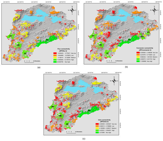
Figure 4.
Different fractions of connectivity between oak forest fragments at the Cuitzeo basin; (a) flux connectivity (dPCfluxk), (b) connector connectivity (dPCconnectork) and (c) intrapatch connectivity (dPCintrak). Levels of importance for the three fractions of connectivity are shown in the figure, its classification was based on the Jenks optimization model. The id of the patches with the highest levels for the three fractions are exhibited in the maps.
4. Discussion
In our study we detected how oak forests fragments in the center of Mexico contribute to maintain regional connectivity. The distribution models for the seven oak species exhibited a high level of predictability, and we detected that half of the area in the basin is a suitable habitat for oak species. We detected differences in the distribution between the oak species, which could be important for maintaining the overall connectivity. In the basin we detected a low level of connectivity between oak forests patches, due to the pressure of extended human activities. However, the oak remnants offered different functions in the connectivity—only one patch due to its size represented a suitable habitat, and the rest of the patches sustained the flux between them and acted as steppingstones. We also detected that the connectivity varied between the regions, particularly the patches at the northern part of the basin were very isolated from the rest. Overall, our results bring forth useful information to guide conservation or restoration actions in the different areas to facilitate the mobility of organisms.
The potential distribution models for seven of the most common oak species in the Cuitzeo Lake basin had moderate to substantial predictability. In particular, the models for Q. rugosa, Q. crassipes, Q. calophylla and Q. castanea were highly accurate, and for the rest of the species, Q. magnoliifolia, Q. deserticola and Q. laeta, predictability was moderate. In the Cuitzeo basin, the oak forests had a large potential area (covering 53% of the basin area), and the largest patches were located in the southern and southeastern portions of the basin. We also detected that oak forest distribution follows environmental gradients. On the one hand, Q. castanea, Q. magnoliifolia, Q. laeta and Q. deserticola were located in the north and center of the basin, a region that has a higher temperature and higher seasonality in the rain pattern. On the other hand, Q. crassipes, Q. rugosa and Q. calophylla were distributed in the south; this area has lower temperature. Our results are in line with the growing evidence exhibiting the distribution of oak species is related with environmental gradients which in part has been attributable to its physiological resistance to stress [31,101,102]. The differences in distribution and physiology between oaks indicates that the ecosystems services that the species provide would be regionally distinct in the landscape, adding to the ecological relevance of the group. Thus, the decisions making to designate conservation areas should include this type of evidence.
We explored if the potential distribution models were related with structural variables (dbh and abundance) of each species; however, we only detected a relationship for Q. calophylla between the dbh and its occurrence values. The lack of association for the rest of the species could be a consequence of the long-term management of oak forest in the area. Historically, in the basin, oak forests have been harvested for firewood and charcoal production [38,64,65]. These activities generate a complex landscape composed of oak forest patches of different ages, with multi-stemmed trees due to the high resprouting capacity of oaks after harvesting cuts [38,43]. In contrast, Q. calophylla within the basin is restricted to the mountain peaks, which makes it less accessible for management practices and is not ideal for charcoal production [43,103]. The lack of correlation between the probability of occurrence and the structural variables for the rest of the species could be a result of the intensive extraction of oak wood in the area.
In general, connectivity between oak forest remnants in the Cuitzeo basin was low. This finding reflects the situation of temperate forests in Mexico that had been deforested by human activities, such as avocado farming [14,17,20,69]. The largest distances between fragments were detected between northern and southern parts of the basin. This low connectivity could be a consequence of different factors. The landscape between the northern and southern oak forest patches is dominated by plains in which extensive modification of the original vegetation has occurred; natural forests have been replaced with agricultural and cattle-raising areas and expanding urban infrastructure with dense population centers [49,66,67,104]. Taken together, these landscape modifications have restricted the movement of potential acorn dispersers, decreasing the levels of connectivity between oak forest patches [89,104]. However, we detected that the connectivity changes between regions within the basin, pointing out the ecological vulnerability for some fragments due to the degree of isolation. The patches in the northern area are in a more critical situation because even between them there is a lack of connection; the most extreme case are the four fragments which are one completely isolated from one other. Based on our results, actions to increase the connectivity can be implemented, such as the establishment of natural corridors between the patches located in this region. In contrast, there is a big corridor of patches going from east to west passing through the south, composed by the biggest fragments in the basin, that without them its connectivity would be reduced substantially. Particularly, in the eastern portion of the basin, the 260 patch with an area of ca. 10,000 hectares contributes almost 50% of the connectivity of the oak remnants and has the largest importance as habitat optimum. In addition, there are four other large-size patches (68, 169, 340 and 467) located in the south and west of the basin, each close to other patches, forming networks and favoring the regional connectivity independently of the dispersal capacity of focal species [105,106]. We detected that some forest fragments preserve connectivity between other regions by acting as steppingstone patches, thereby facilitating the movement of oak dispersers. Steppingstone patches, which offer connectivity to other areas, allow the movement of species to a better-quality habitat, which contributes to maintaining species populations [105,107]. Though, the steppingstone patches in the basin would increase the matrix permeability there are few suitable habitats. This is a recurrent scenario in México, where fragmentation has reduced the large areas and increased the number of small-area patches [3,4,7]. Therefore, particular efforts should be enacted to preserve these large area patches or increase the size of the small ones by restoring vegetation in the vicinity.
In our study, we found numerous small patches that also function as connectors, establishing a large network of oak forest remnants. Most conservation efforts give priority to large patches given their high probability of connectivity with small ones and because they can sustain larger-size populations [108]. Nonetheless, small-area patches are important due to their high complementary capacity by connecting larger patches and defining networks [105,106,109]. Additionally, it has been suggested that conservation and restoration efforts of small patches are more attainable in less time [110,111]. Thus, conservation efforts should also be directed to small steppingstones patches to maintain the overall connectivity of the networks located in the south and southeast of the basin. Particularly, it has been detected that by the combination of extreme environmental conditions within small-area oak patches, pioneers plant species are recruited and cohabit with mature species, which increases species diversity within the patch [44]. This indicates that by directing conservation efforts to small steppingstones patches, regional connectivity and species pool would be favored. On the other hand, areas such as the northern region of the basin where we detected isolated small patches, its importance as steppingstones was very low. Therefore, actions should be implemented to increase the permeability of the matrix in this part of the basin; for example, restoration efforts could be conducted in oak forest remnants that would use oak species to establish living fences in agricultural areas, which could act as corridors [14,112]. The important role of isolated trees in maintaining the genetic connectivity of oak species has been also studied in the fragmented landscape of the Cuitzeo Lake Basin [52]. Oak forests are an important ecosystem that harbor numerous endemic species and contribute to regulate different ecosystem services for humans which are also a relevant resource for local economies [32,33,34,38,39,40,59,60,61,62,63,64,65]. The methodological approach from our study provide evidence to define actions that could contribute to the preservation of such an ecologically relevant ecosystem.
5. Conclusions
Models of distribution had a high degree of prediction and detected that half of the area of the basin is suitable in terms of bioclimatic conditions for oak forest development. Three oak species had a wide distribution, contributing more than other species to the forest remnant connectivity. The connectivity of oak forest remnants in the basin was very low; however, in the south of the basin, there was a network of different-sized patches that may act as important corridors for connecting the adjoining basin. Patches within the basin act as steppingstones and as flux providers, but large size patches representing suitable habitat are scarce. Oak forest remnants may also connect the mixed forests located in the upper parts of the basin with other vegetation types in the lower areas of the basin. Overall, by using the connectivity analysis we were able to detect areas that need conservation and restoration efforts in order to preserve oak forests. Taken together, these results are crucial to define conservation priorities and strategies that promote long-term connectivity.
Author Contributions
Conceptualization, F.P.-G., R.A.-R. and K.O.; methodology, R.A.-R. and A.L.-M.; formal analysis, R.A.-R. and A.L.-M.; investigation, F.P.-G., R.A.-R. and A.L.-M.; writing—original draft preparation, F.P.-G., R.A.-R., K.O. and A.L.-M.; writing—review and editing, F.P.-G., R.A.-R., K.O. and A.L.-M.; visualization, R.A.-R. and A.L.-M.; supervision, F.P.-G. and R.A.-R.; funding acquisition, F.P.-G. All authors have read and agreed to the published version of the manuscript.
Funding
This research was funded by Programa de Apoyo a Proyectos de Investigación e Innovación Tecnólogica (PAPIIT), grant number IA203221.
Institutional Review Board Statement
Not applicable.
Informed Consent Statement
Not applicable.
Data Availability Statement
Not applicable.
Acknowledgments
We acknowledge the technical support provided by Sergio Tinoco Martínez and Gabriela López Barrera.
Conflicts of Interest
The authors declare no conflict of interest. The funders had no role in the design of the study; in the collection, analyses, or interpretation of data; in the writing of the manuscript, or in the decision to publish the results.
References
- Czech, B.; Krausman, P.R.; Devers, P.K. Economic associations among causes of species endangerment in the United States: Associations among causes of species endangerment in the United States reflect the integration of economic sectors, supporting the theory and evidence that economic growth proceeds at the competitive exclusion of nonhuman species in the aggregate. Bioscience 2000, 50, 593–601. [Google Scholar]
- Kerr, J.T.; Deguise, I. Habitat loss and the limits to endangered species recovery. Ecol. Lett. 2004, 7, 1163–1169. [Google Scholar] [CrossRef]
- Santini, N.S.; Adame, M.F.; Nolan, R.H.; Miquelajauregui, Y.; Piñero, D.; Mastretta-Yañes, A.; Cuervo-Robayo, A.P.; Eamus, D. Storage of organic carbon in the soils of Mexican temperate forest. For. Ecol. Mange. 2019, 446, 115–125. [Google Scholar] [CrossRef]
- Prieto-Amparan, J.A.; Villarreal-Guerrero, F.; Martínez-Salvador, M.; Manjarrez-Domínguez, C.; Vázquez-Quintero, G.; Pinedo-Álvarez, A. Spatial near future modeling of land use and land cover changes in the temperate forests of Mexico. PeerJ 2019, 7, e6617. [Google Scholar] [CrossRef] [PubMed]
- Lambin, F.E.; Turner, B.L.; Geist, H.J.; Agbola, S.B.; Angelsen, A.; Bruce, J.W.; Coomes, O.T.; Dirzo, R.; Fisher, G.; Folke, C.; et al. The causes of land-use and land-cover change: Moving beyond the myths. Glob. Environ. Chang. 2001, 11, 261–269. [Google Scholar] [CrossRef]
- Thaden, J.V.; Binnquist-Cervantes, G.; Pérez-Maqueo, O.; Lithgow, D. Half-Century of Forest in a Neotropical Peri-Urban Landscape: Drivers and Trends. Land 2022, 11, 522. [Google Scholar] [CrossRef]
- Legarreta-Miranda, C.K.; Prieto-Amparán, J.A.; Villareal-Guerrero, F.; Morales-Nieto, C.R.; Pinedo-Alvarez, A. Long-Term Land-Use/Land-Cover Change Increased the Landscape Heterogeneity of a Fragmented Temperate Forest Mexico. Forest 2021, 12, 1099. [Google Scholar] [CrossRef]
- Fahrig, L. Effects of habitat fragmentation on biodiversity. Annu. Rev. Ecol. Evol. Syst. 2003, 34, 487–515. [Google Scholar] [CrossRef]
- Haddad, N.M.; Brudvig, L.A.; Clobert, J.; Davies, K.F.; Gonzalez, A.; Holt, R.D.; Lovejoy, T.E.; Sexton, J.O.; Austin, M.P.; Collins, C.D.; et al. Habitat fragmentation and its lasting impact on Earth’s ecosystems. Sci. Adv. 2015, 1, e6617. [Google Scholar] [CrossRef]
- Decocq, G.; Andrieu, E.; Brunet, J.; Chabrerie, O.; De Frenne, P.; De Smedt, P.; Deconchat, M.; Diekmann, M.; Ehrmann, S.; Giffard, B.; et al. Ecosystem services from small forest patches in agricultural landscapes. Curr. For. Rep. 2016, 2, 30–44. [Google Scholar] [CrossRef]
- Wilcove, D.S.; Rothstein, D.; Dubow, J.; Phillips, A.; Losos, E. Quantifying threats to Imperiled Species in the United States. Assessing the relative importance of habitat destruction, alien species, pollution, overexploitation, and disease. BioScience 1998, 48, 607–615. [Google Scholar] [CrossRef]
- Forman, R.T.T. Land Mosaics, the Ecology of Landscapes and Regions; Cambridge University Press: New York, NY, USA, 1995; p. 48. ISBN 978-0-521-47462-7. [Google Scholar]
- Taylor, P.D.; Fahrig, L.; Henein, K.; Merriam, G. Connectivity is a vital element of landscape structure. Oikos 1993, 68, 571–573. [Google Scholar] [CrossRef]
- Correa-Ayram, C.; Mendoza, M.; Pérez-Salicrup, D.; López-Granados, E. Identifying potential conservation areas in the Cuitzeo Lake basin, Mexico by multitemporal analysis of landscape connectivity. J. Nat. Conserv. 2014, 22, 424–435. [Google Scholar] [CrossRef]
- Saura, S. Métodos y herramientas para el análisis de la conectividad del paisaje y su integración en los planes de conservación. In Avances en el Análisis Espacial de Datos Ecológicos: Aspectos Metodológicos y Aplicados; De la Cruz, M., Maestre, F.T., Eds.; ECESPA-Asociación Española de Ecología Terrestre: Móstoles, Spain, 2013; pp. 1–46. ISBN 978-84-616-3448-4. [Google Scholar]
- Kindlmann, P.; Burel, F. Connectivity measures: A review. Landsc. Ecol. 2008, 23, 879–890. [Google Scholar] [CrossRef]
- Molina-Sanchez, A.; Delgado, P.; González-Rodríguez, A.; González, C.; Goméz-Tagle Rojas, A.F.; López-Toledo, L. Spatio-temporal approach for identification of critical conservation areas: A case study with two pine species from a threatened temperate forest in Mexico. Biodivers. Conserv. 2019, 28, 1863–1883. [Google Scholar] [CrossRef]
- Lookingbill, T.R.; Gardner, R.H.; Ferrari, J.R.; Keller, C.E. Combining a dispersal model with network theory to assess habitat connectivity. Ecol. Appl. 2010, 20, 427–441. [Google Scholar] [CrossRef] [PubMed]
- Damschen, E.I.; Haddad, N.M.; Orrock, J.L.; Tewksbury, J.J.; Levey, D.J. Corridors increase plant species richness at large scales. Science 2006, 313, 1284–1286. [Google Scholar] [CrossRef] [PubMed]
- Godínez-Gómez, O.; Cuervo-Robayo, A.P.; Ramírez-Mejía, D.; Tobón, W.; Alarcón, J.; Koleff, P.; Urquiza-Haas, T. Planning landscape connectivity in Mexico under global change. Biodivers. Inf. Sci. Stand. 2019, 3, e6617. [Google Scholar] [CrossRef]
- Bunn, A.G.; Urban, D.L.; Keitt, T.H. Landscape connectivity: A conservation application of graph theory. J. Environ. Manag. 2000, 59, 265–278. [Google Scholar] [CrossRef]
- Correa-Ayram, C.A.; Mendoza, M.E.; Etter, A.; Pérez-Salicrup, D.R. Habitat connectivity in biodiversity conservation: A review of recent studies and applications. Prog. Phys. Geogr. 2016, 40, 7–37. [Google Scholar] [CrossRef]
- Clauzel, C.; Foltête, J.C.; Girardet, X.; Vuidel, G. Graphab 2.0 user manual. Environ. Model. Softw. 2017, 38, 316–327. [Google Scholar]
- Urban, D.; Keitt, T. Landscape connectivity: A graph-theoretic perspective. Ecology 2001, 82, 1205–1218. [Google Scholar]
- Delmas, E.; Besson, M.; Marie-Helene, B.; Burkle, L.A.; Giulio, V.; Riva, D.; Marie-Joseé, F.; Gravel, D.; Guimaraes, P.L., Jr.; Hembry, D.H.; et al. Analyzing ecological networks of species interactions. Biol. Rev. 2019, 94, 16–36. [Google Scholar] [CrossRef] [PubMed]
- Applying Graph Theory in Ecological Research, 1st ed.; Cambridge University Press: Cambridge, UK, 2017; p. 328.
- Layeghifard, M.; Hwang, M.D.; Guttman, D.S. Disentangling Interactions in the Microbiome: A Network Perspective. Trend. Microbiol. 2017, 25, 217–228. [Google Scholar] [CrossRef] [PubMed]
- Valencia-A, S. Diversidad del Género Quercus (Fagaceae) en México. Bol. Soc. Bot. Mex. 2004, 75, 33–53. [Google Scholar] [CrossRef]
- Nixon, K.C. Global Neotropical distribution and diversity of oak (genus Quercus) and oak forest. In Ecology and Conservation of Neotropical Montane Oak Forest; Kappelle, M., Ed.; Springer: Berlin, Germany, 2006; pp. 3–13. ISBN 978-3-540-28909-8. [Google Scholar]
- Morales-Saldaña, S.; De Luna-Bonilla, O.A.; Cadena-Rodríguez, Y.J.; Valencia-A, S. Species distribution of Quercus (Fagaceae) along an altitude gradient, reveals zonation in a hotspot. Bot. Sci. 2021, 99, 722–734. [Google Scholar] [CrossRef]
- Hipp, L.H.; Manos, P.S.; González-Rodríguez, A.; Hanh, M.; Kaproth, M.; McVay, J.D.; Valencia-Avalos, S.; Cavender-Bares, J. Sympatric parallel diversification of major oak clades in the Americas and the origins of Mexican species diversity. New Phytol. 2017, 217, 439–452. [Google Scholar] [CrossRef]
- Villaseñor, J.L. El bosque húmedo de montaña en México y sus plantas vasculares: Catalogo florístico-taxonómico; Comisión Nacional Para el Conocimiento y Uso de la Biodiversidad- Universidad Nacional Autónoma de México: México City, México, 2010; p. 42. ISBN 978-607-02-1557-5. [Google Scholar]
- Uribe-Salas, D.; España-Boquera, M.L.; Torres-Miranda, A. Aspectos biogeográficos y ecológicos del género Quercus (Fagaceae) en Michoacán, México. Act. Bot. Mex. 2019, 126, e1342. [Google Scholar] [CrossRef]
- Chávez-Vergara, B.; García-Oliva, F. Consecuencias funcionales de la diferenciación taxonómica entre secciones del género Quercus: El caso de la reabsorción de nutrientes. Biológicas 2013, 1, 1–7. [Google Scholar]
- Cavender-Bares, J. Diversity, distribution, and ecosystem services of the North American oaks. Int. Oaks 2016, 27, 37–48. [Google Scholar]
- Cavender-Bares, J.; Arroyo, M.T.K.; Abell, R.; Ackerly, D.; Ackerman, D.; Arim, M.; Belnap, J.; Castañeda, M.F.; Dee, L.; Estrada-Carmona, N.; et al. Status and trends of biodiversity and ecosystem functions underpinning nature’s benefit to people. In IPBES the IPBES Regional Assessment Report on Biodiversity and Ecosystem Services for the Americas; Rice, J., Seixas, C.S., Zaccagnini, M.E., Bedoya-Gaitán, M., Valderrama, N., Eds.; Secretariat of the Intergovernmental Science-Policy Platform on Biodiversity and Ecosystem Services: Bonn, Germany, 2018; p. 159. [Google Scholar]
- Rzedowski, J. Vegetacion de Mexico, 1st ed. digital; Comisión Nacional para el Conocimiento y Uso de la Biodiversidad: México City, México, 2006; p. 504. [Google Scholar]
- Aguilar-Romero, R.; Ghilardi, A.; Vega, E.; Skutsch, M.; Oyama, K. Sprouting productivity and allometric relationships of two oak species managed for traditional charcoal making in central Mexico. Biomass Bioenergy 2012, 36, 192–207. [Google Scholar] [CrossRef]
- Castillo-Santiago, M.A.; Ghilardi, A.; Oyama, K.; Hernández-Stefanoni, J.L.; Torres, I.; Flamenco-Sandoval, A.; Fernández, A.; Mas, J.F. Estimating the spatial distribution of woody biomass suitable for charcoal making from remote sensing and geostatistics in central Mexico. Energy Sustain. Dev. 2013, 17, 177–188. [Google Scholar] [CrossRef]
- De la Paz, P.O.; Davalos, S.R.; Cuacuil, G.E. Aprovechamiento de la madera de Encino en Mexico. Madera y Bosques 2000, 6, 3–13. [Google Scholar] [CrossRef][Green Version]
- INEGI (2005) Uso de suelo y vegetación, escala 1:250,000, serie III (continuo nacional).Dirección General de Geografía. Instituto Nacional de Estadística y Geografía. Available online: http://www.conabio.gob.mx/informacion/metadata/gis/usv250ks3gw.xml?_httpcache=yes&_xsl=/db/metadata/xsl/fgdc_html.xsl&_indent=no (accessed on 7 May 2022).
- Asbjornsen, H.; Vogt, K.A.; Ashton, M.S. Synergistic responses of oak, pine and shrub seedlings to edge environments and drought in a fragmented tropical highland oak forest, Oaxaca, Mexico. Ecol. Manag. 2004, 192, 313–334. [Google Scholar] [CrossRef]
- Aguilar-Romero, R.; García-Oliva, F.; Pineda-García, F.; Torres, I.; Peña-Vega, E.; Ghilardi, A.; Oyama, K. Patterns of distribution of nine Quercus species along an environmental gradient in a fragmented landscape in central Mexico. Bot. Sci. 2016, 94, 471–482. [Google Scholar] [CrossRef]
- Aguilar-Santelisses, R.; del castillo, R.F. Factor affecting wood plant species diversity of fragmented seasonally dry oak forest in the Mixteca Alta, Oaxaca, Mexico. Rev. Mex. Biodivers. 2013, 84, 575–590. [Google Scholar] [CrossRef]
- Asbjornsen, H.; Ashton, M.S.; Vogt, D.J.; Palacios, S. Effects of habitat fragmentation on the buffering capacity of edge environments in a seasonally dry tropical oak forest ecosystem in Oaxaca, Mexico. Agric. Ecosyst. Environ. 2004, 103, 481–495. [Google Scholar] [CrossRef]
- Maldonado-López, Y.; Reyes-Cuevas, P.; Stone, G.N.; Nieves-Aldrey, J.L.; Oyama, K. Gall wasp community response to fragmentation of oak tree species: Importance of fragment size and isolated trees. Ecosphere 2015, 6, art31. [Google Scholar] [CrossRef]
- Monterrubio-Rico, T.C.; Charre-Medellin, J.F. López-Ortiz, E.I. Wild felids in temperature forest remnants in an avocado plantation landscape in Michoacán, Mexico. Southwest Nat. 2018, 63, 137–142. [Google Scholar] [CrossRef]
- Mas, J.F.; Velázquez, A.; Díaz-Gallegos, J.R.; Mayorga-Saucedo, R.; Alcántara, C.; Bocco, G.; Castro, R.; Fernández, T.; Pérez-Vega, A. Assessing land use/cover changes: A nationwide multidate spatial database for Mexico. Int. J. Appl. Earth. Obs. Geoinf. 2004, 5, 249–261. [Google Scholar] [CrossRef]
- Mas, J.F.; Lemoine-Rodríguez, R.; González, R.; López-Sánchez, J.; Piña-Garduño, A.; Herrera-Flores, E. Evaluación de las tasas de deforestación en Michoacán a escala detallada mediante un método híbrido de clasificación de imagines SPOT. Madera y Bosques 2017, 23, 119–131. [Google Scholar] [CrossRef]
- Maya-Elizarrarás, E.; Schondube, J.E. Birds, charcoal and cattle: Bird community responses to human activities in an oak forest landscape shaped by charcoal extraction. For. Ecol. Manag. 2015, 335, 118–128. [Google Scholar] [CrossRef]
- Herrera-Arroyo, M.L.; Sork, V.L.; González-Rodríguez, A.; Rocha-Ramírez, V.; Vega, E.; Oyama, K. Seed-mediated connectivity among fragmented populations of Quercus castanea (Fagaceae) in a Mexican landscape. Am. J. Bot. 2013, 100, 1663–1671. [Google Scholar] [CrossRef] [PubMed]
- Oyama, K.; Herrera-Arroyo, M.L.; Rocha-Ramírez, V.; Benítez-Malvido, J.; Ruiz-Sánchez, E.; González-Rodríguez, A. Gene flow interruption in a recently human-modified landscape: The value of isolated trees for the maintenance of genetic diversity in a Mexican endemic red oak. For. Ecol. Manag. 2017, 390, 27–35. [Google Scholar] [CrossRef]
- Ferrusquia-Villafranca, I. Geology of Mexico: A synopsis. In Biological Diversity of Mexico: Origins and Distribution, 1st ed.; Ramamoorthy, T.P., Bye, R., Lot, A., Fa, J., Eds.; Oxford University Press: New York, NY, USA, 1993; pp. 3–107. ISBN 978-0195066746. [Google Scholar]
- Bravo-Espinoza, M.; García-Oliva, F.; Patrón, E.; Mendoza, M.; Camacho, G.; López-Granados, E. La Cuenca del Lago de Cuitzeo: Problemática, Perspectiva y Retos Hacia el Desarrollo Sostenible; Consejo Estatal de Ciencia y Tecnología-Fondo Editorial Morevallado: Morelia, México, 2008; pp. 3–31. ISBN 9789707035782. [Google Scholar]
- Leal-Nares, O.A.; Mendoza, M.E.; Carranza-González, E. Análisis y modelamiento espacial de información climática en la cuenca de Cuitzeo, México. Investig. Geogr. 2010, 72, 49–67. [Google Scholar]
- Morales-Manilla, L.M. Área de Estudio. In Atlas de la Cuenca del Lago de Cuitzeo: Análisis de su Geografía y su Entorno Socioambiental, 1st ed.; Cram, S., Galicia, L., Israde-Alcantara, I., Eds.; Instituto de Geografía-UNAM/Universidad Michoacana de San Nicolás de Hidalgo: México City, México, 2010; pp. 20–23. ISBN 978-607-02-1830-9. [Google Scholar]
- Mendoza, M.; Bocco, G.; López-Granados, E.; Bravo, M. Implicaciones hidrológicas del cambio de la cobertura vegetal y uso del suelo: Una propuesta de análisis espacial a nivel regional en la cuenca cerrada del lago de Cuitzeo, Michoacán. Investig. Geogr. 2002, 49, 92–117. [Google Scholar]
- Maza-Villalobos, S.; Macedo-Santana, F.; Rodríguez-Velázquez, J.; Oyama, K.; Martínez-Ramos, M. Variación de la estructura y composición de comunidades de árboles y arbustos entre tipos de vegetación en la Cuenca de Cuitzeo, Michoacán. Bot. Sci. 2014, 92, 243–258. [Google Scholar] [CrossRef]
- Ramirez-Mejia, D.; Gómez-Tagle, A.; Ghilardi, A. Using aerial photography to estimate wood suitable for charcoal in managed oak forests. Environ. Res. Lett. 2018, 13, 025006. [Google Scholar] [CrossRef]
- De la Cruz, M.C.; Gamboa, J.H.; Sanchez, O.I.A.; Rios, S.J.C.; Rosales, S.R.; Carrillo-Parra, A. Energy characterization of charcoal produced in North Central México. Madera y Bosques 2020, 26, 025006. [Google Scholar] [CrossRef]
- Nygren, A. Community-based forest management within the context of institutional decentralization in Honduras. World Dev. 2005, 33, 639–655. [Google Scholar] [CrossRef]
- Herrera, B.; Chave, A. Criteria and indicators for sustainable management of Central American Montane oak forests. In Ecology and Conservation of Neotropical Montane Oak Forests; Kappelle, M., Ed.; Springer: Berlin, Germany, 2006; pp. 421–434. ISBN 978-3-540-28909-8. [Google Scholar]
- Devia, C.A.; Arenas, H. Evaluacion del estatus ecosistemico y de manejo de los bosques de fagáceas (Quercus humboldtii y Trigomobalanus excelsa) en el norte de la cordillera oriental (Cundinamarca, Santander y Bogota). In Desarrollo Sostenible de Los Andes; Cardenas, F., Ed.; Universidad Javeriana: Colombia, Spain, 1997; pp. 63–77. [Google Scholar]
- Wampamba, T.H.; Ghilardi, A.; Sander, K.; Chaix, K.J. Dispelling common misconceptions to improve attitudes and policy outlook on charcoal in developing countries. Energy Sustain. Dev. 2013, 17, 75–85. [Google Scholar] [CrossRef]
- Camou-Guerrero, A.; Ghilardi, A.; Mwampamba, T.; Serrano, M.; Ortiz-Ávila, T.; Vega, E.; Oyama, K.; Masera, O. Análisis de la producción de carbón vegetal en la Cuenca del Lago de Cuitzeo, Michoacán, México: Implicaciones para una producción sustentable. Investig. Ambient. 2016, 6, 127–138. [Google Scholar]
- Mendoza, M.E.; López-Granados, E.; Geneletti, D.; Pérez-Salicrup, D.R.; Salinas, V. Analyzing land cover and land use change processes at watershed level: A multitemporal study in the Lake Cuitzeo Watershed, Mexico (1975–2003). Appl. Geogr. 2011, 31, 237–250. [Google Scholar] [CrossRef]
- López-Granados, E.; Bocco, G.; Mendoza, M.; Velázquez, A.; Aguirre-Rivera, J.R. Peasant emigration and land-use change at the watershed level: A GIS-based approach in Central Mexico. Agric. Syst. 2006, 90, 62–78. [Google Scholar] [CrossRef]
- Cuervo-Robayo, A.P.; Téllez-Valdés, O.; Gómez-Albores, M.A.; Venegas-Barrera, C.S.; Manjarrez, J.; Martínez-Meyer, E. An update of high resolution monthly climate surfaces for Mexico. Int. J. Climatol. 2014, 34, 2427–2437. [Google Scholar] [CrossRef]
- Correa-Ayram, C.A.; Mendoza, M.E.; Etter, A.; Pérez-Salicrup, D.R. Potential distribution of mountain cloud forest in Michoacán, Mexico: Prioritization for conservation in the context of landscape connectivity. Environ. Manag. 2017, 60, 86–103. [Google Scholar] [CrossRef]
- ESRI, ArcGIS 10.5, Environmental Systems Research Institute: Redlands, CA, USA, 2006.
- Beaumont, L.J.; Hughes, L.; Poulsen, M. Predicting species distributions: Use of climatic parameters in BIOCLIM and its impact on predictions of species´current and future. Ecol. Modell. 2005, 186, 251–270. [Google Scholar] [CrossRef]
- Vasquez-Morales, S.G.; Téllez-Valdés, O.; Pineda-López, R.; Sanchéz-Velásquez, L.R.; Flores-Estevez, N.; Viveros-Viveros, H. Effect of climate change on the distribution of Magnolia schiedeana: A threatened species. Bot. Sci. 2014, 92, 575–585. [Google Scholar] [CrossRef]
- Arenas-Navarro, M.; García-Oliva, F.; Torres-Miranda, A.; Téllez-Valdés, O.; Oyama, K. Environmental filters determine the distribution of tree species in a threatened biodiversity hotspot in western Mexico. Bot. Sci. 2020, 98, 219–237. [Google Scholar] [CrossRef]
- Cobos, M.E.; Townsend-Peterson, A.; Osorio-Olvera, L.; Jiménez-García, G. An exhaustive analysis of heuristic methods for variable selection in ecological niche modeling and species distribution modeling. Ecol. Inform. 2019, 53, 100–983. [Google Scholar] [CrossRef]
- Guisan, A.; Zimmermann, N.E.; Elith, J.; Graham, C.H.; Phillips, S.; Peterson, A.T. What matters for predicting the occurrence of trees: Techniques, data, or species’ characteristics? Ecol. Monogr. 2007, 77, 615–630. [Google Scholar] [CrossRef]
- Maher, S.P.; Randin, C.F.; Guisan, A.; Drake, H.J. Pattern-recognition ecological niche models fit to presence-only and presence-absence data. Methods Ecol. Evol. 2014, 5, 761–770. [Google Scholar] [CrossRef]
- Hallfors, M.H.; Liao, J.; Dzurisin, J.; Grundel, R.; Hyvarinen, M.; Towle, K.; Wu, G.C.; Hellmann, J.J. Addressing potential local adaptation in species distribution models: Implications for conservation under climate change. Ecol. Appl. 2016, 26, 1154–1169. [Google Scholar] [CrossRef] [PubMed]
- Phillips, S.J.; Anderson, R.P.; Schapire, R.E. Maximum entropy modeling of species geographic distributions. Ecol. Modell. 2006, 190, 231–259. [Google Scholar] [CrossRef]
- Elith, J.; Phillips, S.J.; Hastie, T.; Dudik, M.; Chee, Y.E.; Yates, C.J. A statistical explanation of MaxEnt for ecologists. Divers. Distrib. 2011, 17, 43–57. [Google Scholar] [CrossRef]
- Cohen, J. A coefficient of agreement for nominal scales. Educ. Psychol. Meas. 1960, 20, 37–46. [Google Scholar] [CrossRef]
- Wollan, A.K.; Bakkestuen, V.; Kauserud, H.; Gulden, G.; Halvorsen, R. Modelling and predicting fungal distribution patterns using herbarium data. J. Biogeogr. 2008, 35, 2298–2310. [Google Scholar] [CrossRef]
- Maya-García, R.; Torres-Miranda, A.; Cuevas-Reyes, P.; Oyama, K. Morphological differentiation among populations of Quercus elliptica Née (FAGACEAE) along and environmental gradient in Mexico and Central America. Bot. Sci. 2020, 98, 50–65. [Google Scholar] [CrossRef]
- Hirzel, H.A.; Le Lay, G.; Helfer, V.; Randi, C.; Guisan, A. Evaluating the ability of habitat suitability models to predict species presences. Ecol. Modell. 2006, 199, 142–152. [Google Scholar] [CrossRef]
- Webber, M.M.; Stevensen, R.D.; Diniz-Filho, J.A.F.; Grelle, C.E. Is there a correlation between abundance and environmental suitability derived from ecological niche modelling? A meta-analysis. Ecography 2016, 40, 817–828. [Google Scholar] [CrossRef]
- Gomes, H.F.V.; IJFF, D.S.; Raes, N.; Amaral, L.I.; Salomao, P.R.; Cohelo, L.S.; de Almeida Matos, F.D.; Castilho, C.V.; Lima Filho, D.A.; Cardenas, L.D.; et al. Species Distribution Modelling: Contrasting presence-only models with plot abundance data. Sci. Rep. 2018, 8, 1003. [Google Scholar] [CrossRef] [PubMed]
- R Core Team. R: A Language and Environment for Statistical Computing. Available online: http://cran.r-project.org (accessed on 26 October 2019).
- Roy, A.; Bhattacharya, S.; Ramprakash, M.; Kumar, A.S. Modelling critical patches of connectivity for invasive Maling bamboo (Yushania maling) in Darjeelin Himalayas using graph theoretic approach. Ecol. Model. 2016, 329, 77–85. [Google Scholar] [CrossRef]
- Shanthala Devi, B.S.; Murthy, M.S.R.; Debnath, B.; Jha, C.S. Forest patch connectivity diagnostics and priorization using graph theory. Ecol. Model. 2013, 251, 279–287. [Google Scholar] [CrossRef]
- Correa-Ayram, C.A.; Mendoza, M.E.; Etter, A.; Pérez-Salicrup, D.R. Anthropogenic impact on habitat connectivity: A multidimensional human footprint index evaluated in a highly biodiverse landscape of Mexico. Ecol. Indic. 2017, 72, 895–909. [Google Scholar] [CrossRef]
- Sutherland, G.D.; Harestad, A.S.; Price, K.; Lertzman, K.P. Roedores Scaling of Natal Dispersal Distances in Terrestrial Birds and Mammals. Conserv. Ecol. 2000, 4, 16. [Google Scholar]
- Brown, J.L. The Mexican Jay a Model System for the Study of Large Group Size and Its Social Correlates in a Territorial Bird. In Model Systems in Behavioral Ecology Integrating Conceptual, Theoretical, and Empirical Approaches; Dugatkin, L.A., Ed.; Princeton University Press: Oxford, UK, 2001; Volume 70, pp. 338–358. ISBN 0-691-00652-0. [Google Scholar]
- Pesendorfer, M.B.; Sillet, T.S.; Koening, W.D.; Morrison, A.A. Scatter-hoarding corvids as seed dispersers for oaks and pines: A review of widely distributed mutualism and its utility to habitat restoration. Ornithol. Appl. 2016, 118, 215–237. [Google Scholar] [CrossRef]
- Ramos-Palacios, C.R.; Badano, E.I.; Flores, J.; Flores-Cano, J.A.; Flores-Flores, J.L. Distribution patterns of acorns after primary dispersión in a fragmented oak forest and their consequences on predators and dispersers. Eur. J. For. Res. 2014, 133, 391–404. [Google Scholar] [CrossRef]
- Koenig, W.D.; Vuren, D.V.; Hooge, P.N. Detectability, philopatry, and the distribution of dispersal distance in vertebrates. Trends Ecol. Evol. 1996, 11, 514–517. [Google Scholar] [CrossRef]
- López-Barrera, F.; Manson, R.H.; González-Espinoza, M.; Newton, A.C. Effects of the type of montane forest edge on oak seedling establishment along forest-edge-exterior gradients. For. Ecol. Manag. 2006, 225, 234–244. [Google Scholar] [CrossRef]
- Saura, S.; Rubio, L. A common currency for the different ways in which patches and links can contribute to habitat availability and connectivity in the landscape. Ecography 2010, 33, 523–537. [Google Scholar] [CrossRef]
- Saura, S.; Torne, J. Conefor Sensinode 2.2: A software package for quantifying the importance of habitat patches for landscape connectivity. Environ. Model. Softw. 2009, 24, 135–139. [Google Scholar] [CrossRef]
- Saura, S.; Pascual-Hortal, L. A new habitat availability index to integrate connectivity in landscape conservation planning: Comparison with existing indices and application to a case study. Lands Urban. Plan. 2007, 83, 91–103. [Google Scholar] [CrossRef]
- Bodin, Ö.; Saura, S. Ranking individual habitat patches as connectivity providers: Integrating network analysis and patch removal experiments. Ecol. Modell. 2010, 221, 2393–2405. [Google Scholar] [CrossRef]
- Landis, J.R.; Koch, G.G. An application of hierarchical kappa-type statistics in the assessment of majority agreement among multiple observers. Biometrics 1977, 33, 363–374. [Google Scholar] [CrossRef]
- Aguilar-Romero, A.; Pineda-Garcia, F.; Paz, H.; González-Rodríguez, A.; Oyama, K. Differentiation in the water-use strategies among oak species from central Mexico. Tree Physiol. 2017, 37, 915–925. [Google Scholar] [CrossRef]
- Arenas-Navarro, M.; García-Oliva, F.; Terrazas, T.; Torres-Miranda, A.; Oyama, K. Leaf habit and stem hydraulic traits determine functional segregation of multiple oak species along a water availability gradient. Forest 2020, 11, 894. [Google Scholar] [CrossRef]
- Herrera-Fernández, A.C.; Carrillo-Parra, A.; Bucio-Pedraza, F.E.; Correa-Méndez, F.; Herrera-Bucio, R.; López-Albarrán, P.; Rutiaga-Quiñones, J.G. Densidad, composición química y poder calorífico de la madera de tres especies de encinos (Quercus candicans, Q. laurina y Q. rugosa). Cienc. Nicolaita 2017, 72, 136–154. [Google Scholar] [CrossRef]
- Correa-Ayram, C.A.; Mendoza, M.E.; Etter, A.; Pérez-Salicrup, D.R. Effect of the landscape matrix condition for prioritizing multispecies connectivity conservation in a highly biodiverse landscape of Central Mexico. Reg. Environ. Chang. 2019, 19, 149–163. [Google Scholar] [CrossRef]
- Saura, S.; Bodin, Ö.; Fortin, M.J. Stepping stones are crucial for species’ long-distance dispersal and range expansion through habitat networks. J. Appl. Ecol. 2014, 51, 171–182. [Google Scholar] [CrossRef]
- Tulloch, A.I.; Barnes, M.D.; Ringma, J.; Fuller, R.A.; Watson, J.E. Understanding the importance of small patches of habitat for conservation. J. Appl. Ecol. 2016, 53, 418–429. [Google Scholar] [CrossRef]
- Lindenmayer, D. Small patches make critical contributions to biodiversity conservation. Proc. Natl. Acad. Sci. USA 2019, 116, 717–719. [Google Scholar] [CrossRef] [PubMed]
- Cazetta, E.; Fahrig, L. The effects of human-altered habitat spatial pattern on frugivory and seed dispersal: A global meta-analysis. Oikos 2021, 2022, 1–13. [Google Scholar] [CrossRef]
- Fischer, J.; Lindenmayer, D.B. Small patches can be valuable for biodiversity conservation: Two case studies on birds in southeastern Australia. Biol. Conserv. 2002, 106, 129–136. [Google Scholar] [CrossRef]
- Herrera, P.L.; Sabatino, C.M.; Jaimes, R.F.; Saura, S. Landscape connectivity and the role of small habitat patches as stepping stones: An assessment of the grassland biome in South America. Biodivers. Conserv. 2017, 26, 3465–3479. [Google Scholar] [CrossRef]
- Wintle, B.A.; Kujala, H.; Whitehead, A.; Veloz, S.; Kikkala, A.; Moilanen, A.; Gordon, A.; Lentini, P.E.; Cadenhead, N.C.R.; Bekessy, S.A. Global synthesis of conservation studies reveals the importance of small habitat patches for biodiversity. Proc. Natl. Acad. Sci. USA 2019, 116, 909–914. [Google Scholar] [CrossRef] [PubMed]
- Arroyo-Rodríguez, V.; Fahrig, L.; Tabarelli, M.; Watling, J.I.; Tischendorf, L.; Benchimol, M.; Cazetta, E.; Faria, D.; Leal, I.R.; Melo, F.P.L.; et al. Designing optimal human-modified landscapes for forest biodiversity conservation. Ecol. Lett. 2020, 23, 1404–1420. [Google Scholar] [CrossRef]


Publisher’s Note: MDPI stays neutral with regard to jurisdictional claims in published maps and institutional affiliations. |
© 2022 by the authors. Licensee MDPI, Basel, Switzerland. This article is an open access article distributed under the terms and conditions of the Creative Commons Attribution (CC BY) license (https://creativecommons.org/licenses/by/4.0/).