Spatial Prediction Models for Soil Stoichiometry in Complex Terrains: A Case Study of Schrenk’s Spruce Forest in the Tianshan Mountains

Abstract

Spatial patterns of soil carbon (C), nitrogen (N) and phosphorus (P) and their stoichiometric characteristics (C:N:P) play an important role in nutrient limitations, community dynamics, nutrient use efficiency and biogeochemical cycles, etc. To date, the spatial distributions of soil organic C at various spatial scales have been extensively studied, whereas little is known about the spatial patterns of N and P and C:N:P ratios in various landscapes, especially across complex terrains. To fill this gap, we estimated the spatial patterns of concentrations of soil C, N and P and C:N:P ratios in Schrenk’s spruce (Picea schrenkiana Fisch. & C. A. Mey.) forest in the Tianshan Mountains based on data from soil cores collected from 2012 to 2017, and using the following four regression models: multiple linear regression, stepwise regression, ridge regression and lasso regression. We found the following: (1) elevation and climatic variables jointly contributed to concentrations of C, N and P and C:N:P ratios, (2) soil C, N and P concentrations, and their stoichiometric ratios, demonstrated continual spatial patterns in Schrenk’s spruce forest, (3) Multiple linear regression could be reliably used to estimate the spatial patterns of soil elemental concentrations and stoichiometric ratios in mountainous terrain. We suggest that more independent variables (including biotic, abiotic and anthropogenic factors) should be considered in future works. Additionally, adjustment of multiple linear regression and other models should be used for a better delineation of spatial patterns in the concentrations of soil elements and stoichiometric ratios.

1. Introduction

Like those in grasslands and croplands, stocks of macro-nutrients, such as carbon (C), nitrogen (N) and phosphorus (P), in subalpine forests play an important role in the terrestrial biogeochemical cycle, due to their large stocks and potential feedbacks to external disturbances [1,2,3,4]. Since the relative stocks of these nutrients (as well as other nutrients such as potassium, calcium, sodium and magnesium) are crucial for the accumulation and allocation of plant biomass [5,6,7], the science of ecological stoichiometry, which focuses on nutrient ratios and the impact factors of these ratios across different ecosystems, has been proposed [8,9,10]. Currently, ecological stoichiometry has been successfully used to study nutrient limitation [11,12], community dynamics [13,14], microorganism nutrient status [15], symbiosis relationships [16], nutrient use efficiency [17,18] and the biogeochemical cycle [19,20,21] in terrestrial and aquatic ecosystems, and its importance has been widely recognized [22]. However, very few studies have investigated the spatial patterns of variability in nutrient stoichiometry, and the implications of these patterns, on ecosystem functioning. Leroux et al. [23] reported that an improved investigation of the spatial patterns of nutrients and their stoichiometric characteristics may contribute to our understanding of material stocks and fluxes in aquatic and terrestrial ecosystems. To date, some studies have been conducted to delineate the latitudinal and elevational trends in elemental stoichiometry and their climatic drivers. For example, through analysis of foliar and below-ground biomass samples obtained along a Chinese grassland transect, Yu, et al. [24] found that foliar N and P increased with elevation and N and P of below-ground biomass decreased with elevation [24]. In addition, foliar N decreased and below-ground biomass of N increased with MAT [24]. Sardans et al. [25] studied foliar and soil concentrations and the stoichiometry of N and P across European Pinus sylvestris forests and found that Log (N:P) linearly decreased with latitude.

The abovementioned studies shed light on the spatial patterns of nutrients and their stoichiometric ratios in different ecosystems, whereas the corresponding patterns were primarily derived from basic statistical analysis. Specifically, the relationships between concentrations of nutrients and stoichiometric ratios with topographic and climatic variables were obtained based on systematic sampling, Pearson’s correlation and simple linear regression analysis [26,27,28]. These relationships were useful when examining the response of dependent variables (concentrations and stoichiometric ratios) to independent variables (elevation, latitude, MAT, MAP, etc.). However, their application might be restricted, since the spatial variability in the concentrations and stoichiometric ratios across the landscape could not be derived through Pearson’s r and simple linear regression. Fortunately, some attempts that aim to derive the spatial patterns of stoichiometry have been conducted, and valuable results were reported. These methods included geostatistics and spatial interpolation, as reported in Liu et al. [29], in which the authors obtained a spatial distribution map of total soil N and P density across the Loess Plateau of China. Similar work was also reported elsewhere [30,31]. Unfortunately, the successful application of spatial interpolation might be restricted, due to the large number of samples required for accurate spatial estimation, especially in regions with complex topography. In addition, the specific response of concentrations and stoichiometric ratios to determinants cannot be identified. It was reported that remote sensing methods could also be applied for spatial estimation of ecological stoichiometry [32]. However, such a method cannot offer the specific response of concentrations and stoichiometric ratios to determinants. Moreover, the traits of soils beneath the canopy cannot be reliably estimated using remote sensing technologies. Thus, an improved method that could reliably delineate the spatial distribution of nutrient stoichiometric ratios in complex terrains is urgently needed [23].

The Schrenk’s spruce (Picea schrenkiana Fisch. et Mey) forest is a typical subalpine forest in the Tianshan Mountains. The forest ranges from Uzbekistan to northwestern China, spanning more than 2000 km. The broad elevational range (1600–2800 m a.s.l) and unique location of the species offers a unique opportunity to study the spatial distribution of soil C, N, P and C:N:P stoichiometric ratios in subalpine forest. In this study, we conducted statistical analysis to construct a regression (Multiple Linear Regression, MLR, Stepwise Regression, STR, Ridge Regression, RDR, Lasso Regression, LSR) relationship between independent variables (soil C, N, P and C:N:P ratios) and dependent variables (principle components, PCs, of 28 factors include elevation, MAT, MAP, etc.). By applying the regression relationship in our study area, we obtained the spatial distribution of soil C, N, P and C:N:P ratios in the Schrenk’s spruce forest. We hypothesized the following: (1) Soil C, N, P and C:N:P ratios could be delineated using regression approaches and (2) The spatial distribution of soil C, N, P and C:N:P ratios would demonstrate a continuous pattern in the Schrenk’s spruce forest.

2. Materials and Methods

2.1. Study Area

The Tianshan Mountains lie in Central Asia. Our study area (Figure 1) is located in the central and eastern parts of the mountains (42°35′–44°20′ N, 80°14′–88°07′ E) and is characterized by a continental climate, with a cold and dry winter and a warm and humid summer. Due to the unique geographic location and topographic characteristics, the daily temperature range is higher than in surrounding regions. MAT decreases from 13.3 °C at lower elevations (Turpan meteorological station at 30 m a.s.l) to −7.3 °C at higher ones (Shenglidaban at 3600 m a.s.l), while MAP increases from less than 100 mm to over 500 mm with increasing elevation [33]. The maximum temperature of the warmest month, minimum temperature of the coldest month, and precipitation of the wettest quarter range from 10.6 to 30.4 °C, from −29.2 to −17.1 °C and from 36 to 104 mm in the Schrenk’s spruce forest, respectively. Generally, soil in the forest begins to freeze in late November and starts to melt in early April. Spring and autumn are short due to a relatively longer summer and winter. The vegetation types in the Tianshan Mountains include (from low to high elevations) steppe, steppe–forest, subalpine shrubby meadow, alpine–frost action–barren zone, and permanent snow and ice [33]. Schrenk’s spruce forests form single-species stands between 1600 m a.s.l. and 2700 m a.s.l. Shrub species growing at the forest margins include Cotoneaster melanocarpus Lodd., Berberis heteropoda Schrenk., Rosa spinosissima Linn., Spiraea hypericifolia Linn., Juniperus pseudosabina Fisch. & C. A. Mey., Caragana leucophloea Pojark. and Lonicera hispida Pall. ex Roem. et Schult. Understory herbal species include Geranium rotundifolium Linn, Alchemilla tianschanica Juz. and Aegopodium podagraria L. [34].

2.2. Field Sampling and Laboratory Analysis

Fieldwork was conducted in July during 2012–2018. We selected seven sites in the Schrenk’s spruce forest in order to sample the soils, on the basis that these sites have long term meteorological observations (Zhaosu, Jinghe, Shihezi, Baiyanggou, Banfanggou, Shuixigou and Tianchi, as shown in Figure 1 and

Table 1. The topography of sampling sites.

Sampling Site	Average Altitude (m)	Average Slope (°)	Longitude Range (°)	Latitude Range (°)
Zhaosu	2176.65	10.25	80.24–80.49	42.59–42.69
Jinghe	1999.25	16.71	83.17–83.17	44.34–44.35
Qiaoerma	2474.25	9.07	84.28–84.32	43.64–43.64
Shuixigou	2100.63	2.76	87.33–87.34	43.41–43.63
Baiyanggou	2087.09	7.21	87.37–87.39	43.41–43.63
Banfanggou	2018.92	13.01	87.44–87.46	43.43–43.44
Tianchi	2021.20	10.83	88.12–88.12	43.89–43.90

). The stands at these sites are represented by mature forest. At each site, we selected a slope to set up our sampling plots (from lowest elevation to highest one, with approximately 100 m elevational intervals). In total, 171 plots (Table S1) were selected for soil sampling. The longitude, latitude and elevation of each plot were recorded with a global positioning system receiver, i.e., eTrex venture (Garmin Inc., Taiwan, China). Within these plots, we randomly selected 5 points to collect soil cores (using a soil auger). At each point, soils were collected at 0–30 cm, 30–50 cm and 50–80 cm depths. We mixed soils from 5 points to obtain a composite sample for each depth. After being taken to the laboratory, the soil samples were air-dried and sieved for the subsequent chemical analysis. The soil carbon concentration was measured using the potassium dichromate method, as demonstrated in Yeomans and Bremner [35]. Total N concentration (g kg⁻¹) was analyzed using the Kjeldahl digestion method [36]. Total P concentration (g kg⁻¹) was measured using the perchloric acid digestion method, followed by the molybdate colorimetric test [37]. Stoichiometric data were calculated by mass ratio. In order to obtain a value that could represent the stoichiometric characteristics (C, N, P concentrations and C:N ratio, C:P ratio and N:P ratio) of each sampling plot, we calculated the depth weighted average (C, N, P concentrations and C:N ratio, C:P ratio and N:P ratio) of three layers (0–30 cm, 30–50 cm and 50–80 cm).

2.3. Independent Variables

Climate data were obtained from the Worldclim (version 1.4) bioclimatic dataset [38], which provides data as 50-year means for averages and extremes of precipitation and temperature. Based on data collected from more than 40,000 weather stations, climatic variables in the dataset were interpolated using a thin-plate smoothing spline algorithm [38]. The dataset have been successfully used for various spatial modeling applications [39]. We used the resampled (original spatial resolution is 1 km × 1 km and we resampled to 30 m × 30 m) 19 climatic variables (

Table 2. Environmental predictors used to develop spatial distribution of C:N:P ratios in Schrenk’s spruce forest, and principle components analysis (PCA) of these predictors associated with soil stoichiometry. Eigenvalues (and percent of variance) were 12.09 (43.00%), 7.72 (25.75%), 3.01 (10.05%) and 2.14 (7.14%), respectively.

Variable	Abbreviation	Factor Loading
		PC-1	PC-2	PC-3	PC-4
Elevation	ELE	−0.66
Max temperature of warmest month	TWM	0.99
Mean temperature of warmest quarter	TWMQ	0.99
Mean annual temperature	MAT	0.96
Min temperature of coldest month	TCM	0.93
Mean temperature of wettest quarter	TWEQ	0.93
Mean temperature of driest quarter	TDQ	0.90	0.34
Mean temperature of coldest quarter	TCQ	0.90	0.34
Precipitation seasonality	PS	−0.83	−0.41
Precipitation of warmest quarter	PWQ	−0.73	0.63
Mean diurnal range	MDR	0.72	0.65
Precipitation of wettest month	PWM	−0.71	0.63
Precipitation of wettest quarter	PWQ	−0.70	0.66
Soil pH	pH	0.64	−0.44		0.41
Temperature annual range	TAR	0.63			0.55
Coarse fragments percentage	CRF	−0.60	0.51	−0.34
Cation exchange capacity	CEC	−0.60		0.36
Mean annual precipitation	MAP	−0.33	0.90
Precipitation of driest quarter	PDQ		0.88		0.36
Precipitation of coldest quarter	PCQ		0.88		0.36
Precipitation of driest month	PDM		0.85		0.39
Temperature seasonality	TS	−0.38	−0.78		0.45
Isothermality	ISO	0.60	0.73		−0.30
Sand content	SDC		0.47	−0.84
Clay content	CLC		−0.39	0.77
Silt content	STC		−0.42	0.74
Bulk density	BD	0.52
Available soil water capacity	AWC	0.41	−0.36	−0.31	0.34

) in the dataset to delineate the climate condition of our study area. Although some of the variables are highly correlated, they were all used in ecological modelling [40,41]. Therefore, these 19 climatic variables were also included in our independent variables dataset. The considered independent variables also included elevation, available soil water capacity (AWC, volumetric fraction), bulk density (BD, g cm⁻³), cation exchange capacity (CEC, cmolc kg⁻¹), clay content (CLC, mass fraction in %), coarse fragments (CRF, volumetric in %), soil pH (pH), silt content (STC, mass fraction in %), sand content (SDC, mass fraction in %). These soil predictors (AWC, BD, CEC, CLC, CRF, pH, STC and SDC, Table 2) were extracted from the SoilGrids dataset, which provides global predictions (based on globally fitted models using soil core and environmental covariate data) for standard numeric soil properties [42]. Since principal component analysis (PCA) is a useful dimension-reduction method, it was used in this study to find principal components (PCs) of these 28 variables (Table 2).

2.4. Actual Distribution of the Schrenk’s Spruce Forest and Spatial Estimation of C, N, P Concentration and C:N:P Ratio

The abovementioned field sampling and corresponding laboratory analysis provided the data to calculate soil C, N and P stoichiometric characteristics (also including the C, N and P concentrations and stoichiometric ratio among the three elements). The actual distribution of the Schrenk’s spruce forest was necessary for spatial estimation of C, N, and P stoichiometric characteristics in the forest. In this study, the actual distribution of the Schrenk’s spruce forest was extracted from a dataset compiled by Hou, et al. [43] and obtained from the Environmental and Ecological Science Data Center for West China (http://westdc.westgis.ac.cn (accessed on 16 July 2018)). The original vector data were first converted to raster format using a conversion tool and, subsequently, resampled to 30 m × 30 m resolution. The spatial distributions of soil C, N and P concentrations and C:N:P were predicted using the constructed regression models (MLR, STR, SDR and LSR). MLR constructed the regression relationship between dependent and independent variables as:

$$Y={\beta }_0+{\beta }_1{X}_1+{\beta }_2{X}_2+\dots +{\beta }_k{X}_k+\epsilon$$

(1)

where $Y$ is the dependent variables (C, N, and P concentrations and C:N:P ratios), $\beta s$ are the regression coefficients of independent variables (PCs) $Xs$, and $\epsilon$ is the error. MLR is the extension of ordinary least-squares (OLS) regression because it involves more than one explanatory variable.

STR carried out the selection of predictive variables in each step by including or excluding variables from the explanatory variables set, based on a specified criterion. In this study, we used the forward selection approach, which starts with no variables (PCs) and adds variables (PCs), the inclusion of which improve the performance of the fitting. STR is faster than other automatic model-selection methods and allows observation of the order in which variables are removed or introduced, which might provide useful information about the independent variables’ qualities.

RDR added a regularization term to the squared residuals of ordinary least squares. Being a supplement of the least square method, RDR improves the condition of the considered regression problem and enables a direct numerical solution. Therefore, RDR is an efficient regression technique that is used when multicollinearity exist or when the number of predictor variables in a set exceed the number of observations.

Similar to RDR, LSR also shrinks the regression coefficients towards zero via a regularization term so that the variance can be substantially reduced, which leads to a lower overall Mean Squared Error [44].

Since MLR and RDR could not shrink the regression coefficients towards zero (i.e., large number of independent variables), we used PCs as the independent variables for these two approaches. In contrast, all the 28 variables were used for STR and LSR.

The performances of these models were evaluated using mean absolute error (MAE), root mean square error (RMSE), and adjusted coefficient of determination (R²). These indices were calculated as follows:

$$MAE=\frac{100}{n}{\displaystyle \sum }_{t=1}^n\left|\frac{F_t-A_t}{A_t}\right|$$

(2)

$$RMSE=\sqrt{\frac{1}{n}{\displaystyle \sum }_{t=1}^N{\left(F_t-A_t\right)}^2}$$

(3)

$${\overline{R}}^2=1-\left(1-\frac{{{\displaystyle \sum }}_{t=1}^N{\left(F_t-\overline{A}\right)}^2}{{{\displaystyle \sum }}_{t=1}^N{\left(A_t-\overline{A}\right)}^2}\right)\left(\frac{n-1}{n-k-1}\right)$$

(4)

$$F=\frac{SSR/k}{SSE/\left(n-k-1\right)}$$

(5)

$$\mathrm{SSR}={\left(F_t-\overline{A}\right)}^2$$

(6)

$$\mathrm{SSE}={\left(A_t-F_t\right)}^2$$

(7)

where $A_t$ denotes the actual value, $F_t$ is the modeled value, $\overline{A}$ is the average of actual value, $n$ and $k$ are sample size and number of independent variables in the regression model. Regression models were considered significant if the calculated F-value was greater than the threshold value at a 0.05 significance level. MLR, STR and SDR were carried out using SPSS (IBM SPSS Statistics, Chicago, IL, USA, version 22.0) and regression coefficients of LSR were obtained using the glmnet package in R [45].

3. Results

3.1. Statistics of Soil C, N and P Concentrations and C:N:P Stoichiometric at Sampling Sites

At our sampling sites, the ranges of C, N and P concentrations were 3.12–139.94 g kg⁻¹, 1.78–16.23 g kg⁻¹ and 0.37–1.46 g kg⁻¹, with averages of 55.76 (±25.24) g kg⁻¹, 4.63 (±2.11) g kg⁻¹ and 0.71 (±0.21) g kg^{−1 (}

Table 3. Statistics of soil ecological stoichiometry at sampling sites.

Sample Sites		C (g kg−1)	N (g kg−1)	P (g kg−1)	C:N	C:P	N:P
Zhaosu	Min	48.28	3.10	0.42	7.50	42.83	6.05
	Max	122.59	12.22	1.13	15.89	161.71	19.39
	Mean	71.80	6.19	0.74	12.40	104.45	11.48
Jinghe	Min	3.12	1.83	0.46	1.34	3.26	2.00
	Max	54.57	5.42	1.20	14.17	84.26	11.39
	Mean	33.57	3.48	0.81	9.64	45.65	5.25
Qiaoerma	Min	24.89	2.64	0.38	7.02	32.39	3.92
	Max	79.30	5.74	1.25	20.65	129.43	11.59
	Mean	64.20	4.69	0.83	14.02	80.64	7.16
Shuixigou	Min	32.44	3.10	0.37	8.62	60.29	7.16
	Max	139.94	16.23	1.10	14.73	150.66	13.25
	Mean	72.81	6.06	0.66	12.65	108.27	10.56
Baiyanggou	Min	20.49	2.03	0.37	6.07	41.84	4.10
	Max	84.20	6.69	0.93	14.21	140.49	11.16
	Mean	50.11	4.31	0.69	11.50	71.72	7.06
Banfanggou	Min	10.42	1.78	0.38	4.20	17.12	2.85
	Max	79.46	7.64	1.06	12.41	90.68	28.17
	Mean	51.38	4.73	0.71	10.64	68.84	9.86
Tianchi	Min	24.16	2.00	0.38	7.96	37.13	3.35
	Max	77.29	6.09	0.80	17.36	119.86	10.57
	Mean	48.16	3.90	0.57	12.44	84.09	7.29

). The C:N, C:P and N:P stoichiometric ratios ranged from 1.33 to 31.15, from 2.26 to 172.70 and from 1.99–28.16, with averages of 12.24, 79.95 and 28.16, respectively (Table 3). In contrast, the C:N, C:P and N:P ratios had relatively higher variability with standard deviation of ±3.73, ±31.89 and ±3.18, respectively, compared with their mean values.

3.2. Principal Components of Predictors

According to PCA, the first four PCs accounted for 85.93% of the total variation in the selected predictors (28 in total,

Table 4. Total variance explained by each PC.

Component	Initial Eigenvalues
	Total	% of Variance	Cumulative %
Elevation	12.900	42.999	42.999
Max temperature of warmest month	7.724	25.748	68.746
Mean temperature of warmest quarter	3.014	10.048	78.794
Mean annual temperature	2.142	7.140	85.934
Min temperature of coldest month	1.395	4.649	90.583
Mean temperature of wettest quarter	1.151	3.838	94.421
Mean temperature of driest quarter	0.509	1.696	96.117
Mean temperature of coldest quarter	0.355	1.183	97.300
Precipitation seasonality	0.299	0.998	98.298
Precipitation of warmest quarter	0.134	0.446	98.744
Mean diurnal range	0.119	0.396	99.140
Precipitation of wettest month	0.079	0.264	99.404
Precipitation of wettest quarter	0.068	0.225	99.629
Soil pH	0.043	0.142	99.771
Temperature annual range	0.024	0.081	99.852
Coarse fragments percentage	0.016	0.055	99.907
Cation exchange capacity	0.011	0.036	99.943
Mean annual precipitation	0.009	0.029	99.972
Precipitation of driest quarter	0.004	0.015	99.987
Precipitation of coldest quarter	0.002	0.008	99.995
Precipitation of driest month	0.001	0.002	99.997
Temperature seasonality	0.000	0.001	99.998
Isothermality	0.000	0.001	99.998
Sand content	0.000	0.001	99.999
Clay content	0.000	0.000	99.999
Silt content	7.261 × 10−5	0.000	100.000
Bulk density	6.221 × 10−5	0.000	100.000
Available soil water capacity	4.683 × 10−5	0.000	100.000

). Among these four PCs, the first PC primarily described the temperature-related predictors, and the second and third PCs mainly correlated with precipitation and soil properties (Table 2).

3.3. Model Performance and Correlation between C:N:P Stoichiometrics and Environmental Variables

The predictive performance evaluated by correlation coefficient between observed and modeled value, the adjusted R², MAE and RMSE are displayed in

Table 5. Summary of regression models.

Model	Independent Variables	Performance of Models with Original 28 Variables				Performance of Models with PCs
		Adjusted R2	F	MAE (%)	RMSE	Adjusted R2	F	MAE (%)	RMSE
MLR	C	0.20	1.93 *	41.69	21.60	0.09	2.54 *	44.27	22.64
	N	0.31	2.58 **	97.72	0.17	0.32	8.58 **	86.98	0.17
	P	0.39	3.05 **	33.50	0.04	0.21	4.92 **	46.96	0.06
	C:N	0.51	4.01 **	80.40	13.51	0.04	1.62	49.70	12.92
	C:P	0.12	1.26	21.67	47.64	0.03	1.02	21.69	45.00
	N:P	0.15	1.61	42.36	1.89	0.14	4.35 **	34.90	1.86
STR	C	0.13	12.77 **	56.92	23.17	0.05	5.12 *	45.18	22.06
	N	0.34	14.25 **	77.87	0.16	0.31	19.04 **	90.95	0.17
	P	0.29	16.30 **	86.64	0.09	0.22	8.04 **	43.77	0.06
	C:N	0.12	9.02 **	45.87	12.59	0.03	1.96	43.29	13.37
	C:P	0.05	4.91 *	22.29	46.62	0.02	1.01	21.71	45.05
	N:P	0.21	10.17 **	43.49	1.53	0.13	13.18 **	49.25	1.80
RDR	C	0.22	2.44 **	54.54	22.53	0.06	2.19	44.11	22.12
	N	0.26	2.73 **	66.94	0.19	0.33	10.65 **	94.77	0.17
	P	0.38	3.71 **	65.89	0.07	0.17	4.71 **	41.11	0.05
	C:N	0.37	3.47 **	75.64	18.74	0.04	1.77	43.61	13.28
	C:P	0.10	1.10	20.60	44.63	0.02	0.98	22.40	46.17
	N:P	0.20	2.29 **	48.81	1.79	0.15	5.84 **	55.35	1.72
LSR	C	0.20	1.93 *	66.97	22.50	0.10	3.17 *	47.95	26.62
	N	0.32	2.77 **	72.21	0.18	0.10	3.15 *	90.14	0.17
	P	0.39	3.14 **	71.06	0.08	0.22	6.09 **	45.91	0.06
	C:N	0.51	4.14 **	72.48	13.78	0.04	1.90	52.19	12.97
	C:P	0.13	1.29	22.28	49.15	0.03	1.02	23.04	47.22
	N:P	0.13	1.61	69.31	1.78	0.14	5.76 **	45.63	1.77

Notes: * indicate p < 0.05, ** indicate p < 0.01. PC: principal component of original 28 variables. MAE, mean absolute error; RMSE, root mean square error; MLR: multiple linear regression; STR, Stepwise Regression; RDR, Ridge Regression; LSR, Lasso Regression.

. The range of F value (1.93–19.04) suggested that the four models (MLR, STR, RDR and LSR) were highly predictive when used to fit the linear regression relationship between observed and modeled concentrations of soil C, N and P. In contrast, relatively poorer prediction capability could be found when these models were used to delineate the linear relationship between observed and modeled ratios of C:N, C:P and N:P (especially the C:P ratios, Table 5). In general, the MLR model outperformed the other models, as indicated by the higher adjusted R² and F value. Additionally, according to adjusted R², these models had higher explanatory capacity regarding the variation of concentrations of soil C, N and P and C:N:P stoichiometry when using the original 28 predictors (adjusted R² from 5%–51% with an average of 25.13%), compared with the PCs (adjusted R² from 2%–33% with an average of 12.46%).

The correlation coefficients (r) were also calculated in order to evaluate the correlation relationship between concentrations of soil C, N and P and C:N:P stoichiometry with environmental variables. Corresponding results revealed that soil C concentration had a relatively higher positive r with pH and temperature annual range, and negative r with precipitation seasonality and precipitation of the wettest quarter. N concentration had higher r with temperature seasonality, isothermality and coarse fragments percentage. Mean diurnal range, isothermolity, precipitation seasonality, and precipitation of the wettest quarter were the four variables having higher r with P concentration. Precipitation seasonality, clay content and sand content highly correlated with C:N ratios. For C:P ratios, only the available soil water capacity obtained an r higher than 0.2 (0.26), while all the other variables including PCs were poorly correlated with the ratios. The variables with relatively higher r with N:P ratios included coarse fragment percentage, temperature annual range and temperature seasonality.

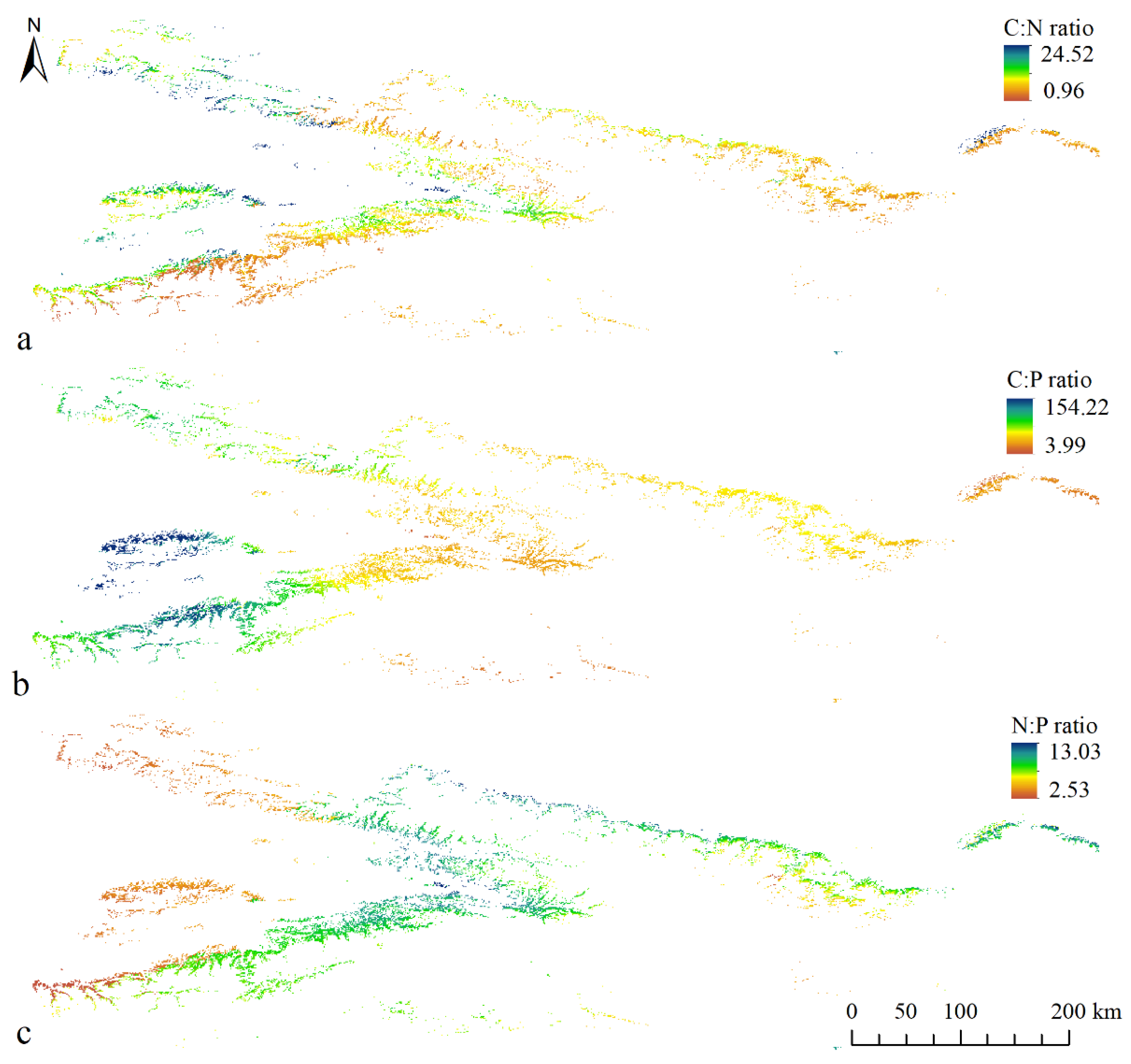
3.4. Spatial Patterns of Soil C, N and P Concentrations and C:N:P Ratios

Figure 2 and Figure 3 show the modeled spatial distribution of soil C, N and P concentrations and C:N:P ratios using the models listed in Table 5. Only the spatial distributions with highest adjusted-R² are displayed. As shown in the figures, measured C concentrations ranged from 3.12 to 139.94 g kg⁻¹ with an average of 55.76 g kg⁻¹. The modeled range was 24.72–83.96 g kg⁻¹ with an average of 53.15 g kg⁻¹ (Figure 2). Standard deviation (SD) of the modeled value was lower than that of the measured ones. The modeled N concentration (0.11–0.53 g kg⁻¹) had a relatively narrower range than the measured values. Similar to SD of the C concentration, the modeled N concentration also had lower variation than the measured value with relatively lower SD. For P concentration, a relatively wider range was found in modeled values (0.26–1.58 g kg⁻¹) than measured values (0.37–1.46 g kg⁻¹), which also resulted in a relatively higher average concentration (0.73 g kg⁻¹ compared to 0.71 g kg⁻¹). The SD of the modeled P concentration was higher than that of the measured value. The average values and SD of the modeled C:N ratio (45.36 and 20.58, Figure 3) were lower than the measured ones (average of 55.76 and SD of 25.24). C:P and N:P ratios in the modeled results had narrower ranges than those of the measured values. In addition, the modeled averages of the two ratios were higher than those of the measured ones. As in the other estimations, the SDs of these two ratios in the modeled results were lower than those of the measured data (Figure 2 and Figure 3).

C concentration was highest in the eastern part of the study area, while the central and southwestern parts corresponded to relatively lower C concentrations (Figure 2a). The northwestern study area also had a relatively higher C concentration. N concentration displayed an opposing trend with C concentration, in that there was a relatively lower concentration in the eastern study area, while the southwestern part had a relatively higher concentration (Figure 2b). The trend in the P concentration was similar to that of the C concentration, and increased from west to east in the study area (Figure 2c). C:N ratios showed a complex pattern in the western part of the study area, whereas, generally, the ratios decreased from west to east, as illustrated in Figure 3a. C:P ratios showed a spatial pattern similar to that of the C:N ratios (Figure 3b). In contrast with the overall trend of C:N and C:P ratios, N:P ratios were lower in the west, higher in the east, and exhibited an increasing trend from the western to eastern parts of the study area (Figure 3c).

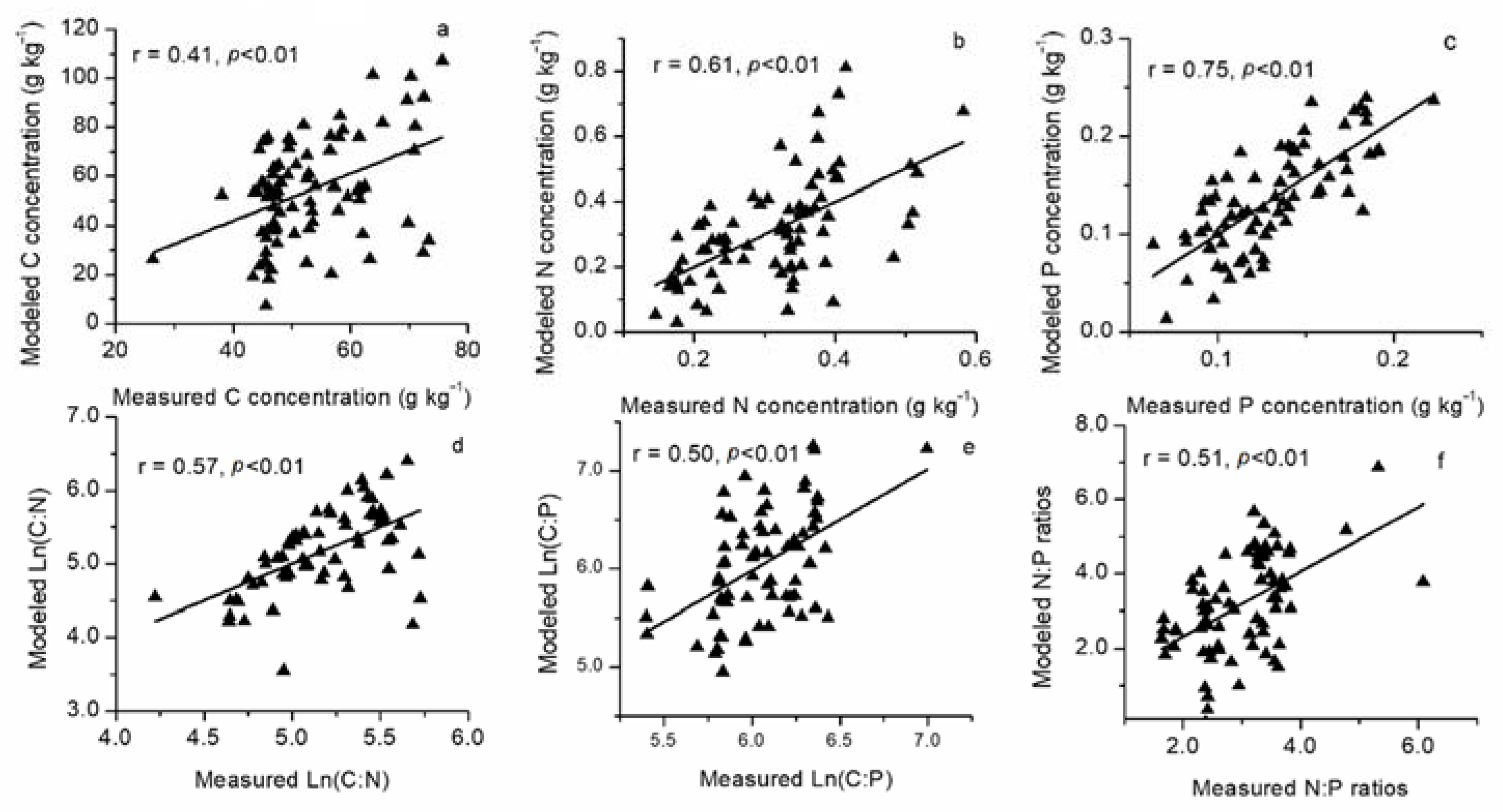
3.5. Comparison between Measured and Modeled Values

The correlation coefficient (r) between actual and modeled C concentration was 0.41 (p < 0.01, Figure 4a). The majority of measured C concentrations were higher than 40 g kg⁻¹, whereas, as shown in Figure 4a, more scatters with modeled values lower than 40 g kg⁻¹ appeared, indicating restricted performance of the multiple regression model. Relatively higher r (0.61) with a high confidence level (p < 0.01) between measured and modeled N concentrations (Figure 4b) suggested reliability of the N concentration model compared with the C model. The r between measured and modeled values of P concentration was highest among the C, N and P concentrations at 0.75 (p < 0.01, Figure 4c), indicating that the P model was the most reliable among the three concentration models. Figure 4d displays the scatter of measured and modeled Ln (C:N) at our sampling sites, A correlation coefficient of 0.57 with 0.01 significance level between measured and modeled Ln (C:N) suggested the reliability of the model, whereas the scatters at the lower-right corner indicated the moderate confidence of the model to the higher values of the C:N ratios. Moderate and significant r values (0.51 and p < 0.01) between measured and modeled values of Ln (C:P) were partly impacted by the restricted estimation of the median value of the C:P ratios, as displayed in Figure 4e. The performance of the N:P ratios model was also acceptable, as shown in Figure 4f.

4. Discussion

4.1. Spatial Patterns of C, N and P Concentrations and C:N:P Stoichiometry in the Schrenk’s Spruce Forest

We hypothesized that the spatial distribution of soil C, N, P and C:N:P ratios would demonstrate a continuous pattern in the Schrenk’s spruce forest. As demonstrated in Figure 3 and Figure 4, C and P concentrations and N:P ratios increased from west to east within the study area, while N concentration and the other two ratios (C:N and C: P) decreased along the west–east direction. A previous investigation by Dai et al. [46] revealed similar variations in soil organic C and total N at sampling sites distributed from west to east in the Tianshan Mountains. According to their results, the differences in soil nutrient concentrations were caused by variations in abiotic variables, including temperature, precipitation, evaporation capacity and solar radiation. In addition, a systematic soil survey conducted in the Tianshan Mountains reported relatively lower concentrations of soil C and P in the eastern part of the study area compared with the western part [47]. It should be noted that the comparison of the concentrations and stochiometric ratios of previous studies were conducted among sampling sites. In contrast, our study not only confirmed the general variations in the concentrations of elements and their stochiometric ratios, but also provided the spatial patterns or variations of the concentrations and stochiometric ratios based on the data derived from sampling sites. In fact, these spatial patterns are more useful for a better understanding of the regional biological and ecological processes corresponding to soil chemical characteristics [23,48].

4.2. Reliability of MLR Models

Ecological stoichiometry plays an important role in nutrient limitation [11,12], nutrient use efficiency [17], community dynamics [13], symbiosis relationship [16] and regional and global biogeochemical cycles [19,20]. However, very few studies have investigated the spatial patterns of variability in nutrient stoichiometry and the implications of these patterns on ecosystem functioning. Recently, stoichiometric distribution models (StDMs), which imitate the species distribution model and aim to delineate the spatial pattern of elemental stoichiometry, were developed and used to map spatial structures in resource elemental composition and the response of consumers across a landscape [23]. Similar to our approach, the StDMs also fitted generalized linear regression models between elemental response variables and covariates. According to their results, StDMs allow researchers to map elemental resources across geographic spaces and hold the promise of describing geographical patterns in organismal elemental traits at various spatial extents [23]. In this study, we found that the R² of the MLR models were high (Table 5), further supporting the reliability of MLR models in spatial estimation of elemental concentrations and stoichiometric ratios. In addition, Rial et al. [49] also reported good predictive performance of MLR when estimating soil C concentration in NW Spain.

4.3. Advantages and Limitations of MLR

Here, we document the potential application of MLR in spatial estimation of elemental concentrations and stoichiometry. Through modeling the spatial distribution of concentrations of C, N and P and their stoichiometric ratios in Schrenk’s spruce forest, we identified the following advantages of the MLR model: (1) the responses of concentrations and stoichiometric ratios to independent variables could be reliably quantified using the model, (2) the regression parameters of the model could be easily estimated using data obtained from collected samples, (3) the spatial variations in the concentrations and stoichiometric ratios could be delineated using geographic information systems platforms, and (4) the modeled results were reliable according to corresponding evaluation (Table 5 and Figure 4).

While MLR is only one of the approaches that enable spatial estimation, other models have potential in similar applications, and obvious limitations of MLR models also exist when compared with other spatial delineation methods. For example, artificial neural networks (ANN) have the ability to detect complex nonlinear relationships between dependent and independent variables and possible interactions between predictor variables [50]. In multivariate adaptive regression splines (MARS), interactions between variables can be fitted, and, rather than fitting a global interaction between a pair of variables, the interactions are specified locally using basis functions [30]. Classification and regression trees (boosted regression trees, random forests, etc.) are a valuable addition to statistical approaches for the analysis of complex ecological data due to their invariance to transformations of explanatory variables and procedures for handling missing values [31]. Genetic algorithms (GA) are a global optimization method that mimic the action of natural selection to solve complex optimization problems and provide a very efficient method of convergence towards the ideal solution [51].

5. Conclusions

In summary, we estimated the spatial patterns of concentrations of C, N and P and their stoichiometric ratios in Schrenk’s spruce forest in the Tianshan Mountains of China. The corresponding results demonstrated the importance of developing reliable methods to delineate the spatial distributions of nutrient concentrations and stoichiometric characteristics. The results have considerable relevance for studies on regional biogeochemical cycles, particularly in complex terrains. We conclude that the concentrations of C, N and P and their stoichiometric ratios in Schrenk’s spruce forest could be accurately estimated use MLR methods and that future works can be improved with more independent variables (biotic, abiotic and anthropogenic factors), with adjustment of MLR models, or with implementation of other models (ANN, MARS, GA) that have been successfully adopted for the spatial estimation of soil organic C.

References

1. Allison, S.D.; Treseder, K.K. Warming and drying suppress microbial activity and carbon cycling in boreal forest soils. Glob. Chang. Biol. 2008, 14, 2898–2909. [Google Scholar] [CrossRef]
2. Huang, W.; Schoenau, J. Forms, amounts and distribution of carbon, nitrogen, phosphorus and sulfur in a boreal aspen forest soil. Can. J. Soil Sci. 1996, 76, 373–385. [Google Scholar] [CrossRef]
3. Cao, Y.; Chen, Y. Ecosystem C: N: P stoichiometry and carbon storage in plantations and a secondary forest on the Loess Plateau, China. Ecol. Eng. 2017, 105, 125–132. [Google Scholar] [CrossRef]
4. Ouyang, S.; Xiang, W.; Gou, M.; Lei, P.; Chen, L.; Deng, X.; Zhao, Z. Variations in soil carbon, nitrogen, phosphorus and stoichiometry along forest succession in southern China. Biogeosci. Disc. 2017, 1–27. [Google Scholar] [CrossRef]
5. Lie, G.; Xue, L. Biomass allocation patterns in forests growing different climatic zones of China. Trees 2016, 30, 639–646. [Google Scholar] [CrossRef]
6. Niinemets, Ü. Responses of forest trees to single and multiple environmental stresses from seedlings to mature plants: Past stress history, stress interactions, tolerance and acclimation. For. Ecol. Manag. 2010, 260, 1623–1639. [Google Scholar] [CrossRef]
7. Buchkowski, R.W.; Shaw, A.N.; Sihi, D.; Smith, G.R.; Keiser, A.D. Constraining carbon and nutrient flows in soil with ecological stoichiometry. Front. Ecol. Evol. 2019, 382. [Google Scholar] [CrossRef]
8. Elser, J.; Sterner, R.; Gorokhova, E.a.; Fagan, W.; Markow, T.; Cotner, J.; Harrison, J.; Hobbie, S.; Odell, G.; Weider, L. Biological stoichiometry from genes to ecosystems. Ecol. Lett. 2000, 3, 540–550. [Google Scholar] [CrossRef]
9. Sterner, R.W.; Elser, J.J. Ecological stoichiometry. In Ecological Stoichiometry; Princeton University Press: Princeton, NJ, USA, 2017. [Google Scholar]
10. McGroddy, M.E.; Daufresne, T.; Hedin, L.O. Scaling of C: N: P stoichiometry in forests worldwide: Implications of terrestrial redfield-type ratios. Ecology 2004, 85, 2390–2401. [Google Scholar] [CrossRef]
11. Feller, I.C.; McKee, K.L.; Whigham, D.F.; O’neill, J.P. Nitrogen vs. phosphorus limitation across an ecotonal gradient in a mangrove forest. Biogeochemistry 2003, 62, 145–175. [Google Scholar] [CrossRef]
12. Högberg, P.; Näsholm, T.; Franklin, O.; Högberg, M.N. Tamm Review: On the nature of the nitrogen limitation to plant growth in Fennoscandian boreal forests. For. Ecol. Manag. 2017, 403, 161–185. [Google Scholar] [CrossRef]
13. Johnson, M.T.; Agrawal, A.A. Plant genotype and environment interact to shape a diverse arthropod community on evening primrose (Oenothera biennis). Ecology 2005, 86, 874–885. [Google Scholar] [CrossRef]
14. Qi, K.; Pang, X.; Yang, B.; Bao, W. Soil carbon, nitrogen and phosphorus ecological stoichiometry shifts with tree species in subalpine plantations. PeerJ 2020, 8, e9702. [Google Scholar] [CrossRef]
15. Hill, B.H.; Elonen, C.M.; Seifert, L.R.; May, A.A.; Tarquinio, E. Microbial enzyme stoichiometry and nutrient limitation in US streams and rivers. Ecol. Indic. 2012, 18, 540–551. [Google Scholar] [CrossRef]
16. Mariotte, P.; Canarini, A.; Dijkstra, F.A. Stoichiometric N: P flexibility and mycorrhizal symbiosis favour plant resistance against drought. J. Ecol. 2017, 105, 958–967. [Google Scholar] [CrossRef]
17. He, W.-M.; Yu, F.-H.; Zhang, L.-L. Physiological integration impacts nutrient use and stoichiometry in three clonal plants under heterogeneous habitats. Ecol. Res. 2010, 25, 967–972. [Google Scholar] [CrossRef]
18. Di Palo, F.; Fornara, D.A. Plant and soil nutrient stoichiometry along primary ecological successions: Is there any link? PLoS ONE 2017, 12, e0182569. [Google Scholar]
19. Schmidt, S.; Porazinska, D.; Concienne, B.-L.; Darcy, J.; King, A.; Nemergut, D. Biogeochemical stoichiometry reveals P and N limitation across the post-glacial landscape of Denali National Park, Alaska. Ecosystems 2016, 19, 1164–1177. [Google Scholar] [CrossRef]
20. Midgley, M.G.; Phillips, R.P. Resource stoichiometry and the biogeochemical consequences of nitrogen deposition in a mixed deciduous forest. Ecology 2016, 97, 3369–3378. [Google Scholar] [CrossRef]
21. Rahman, M.; Zhang, K.; Wang, Y.; Ahmad, B.; Ahmad, A.; Zhang, Z.; Khan, D.; Muhammad, D.; Ali, A. Variations in soil physico-chemical properties, soil stocks, and soil stoichiometry under different soil layers, the major forest region Liupan Mountains of Northwest China. Braz. J. Biol. 2022, 84. [Google Scholar] [CrossRef]
22. Feng, M.; Zhang, D.; He, B.; Liang, K.; Xi, P.; Bi, Y.; Huang, Y.; Liu, D.; Li, T. Characteristics of soil C, N, and P stoichiometry as affected by land use and slope position in the Three Gorges Reservoir Area, southwest China. Sustainability 2021, 13, 9845. [Google Scholar] [CrossRef]
23. Leroux, S.J.; Wal, E.V.; Wiersma, Y.F.; Charron, L.; Ebel, J.D.; Ellis, N.M.; Hart, C.; Kissler, E.; Saunders, P.W.; Moudrá, L. Stoichiometric distribution models: Ecological stoichiometry at the landscape extent. Ecol. Lett. 2017, 20, 1495–1506. [Google Scholar] [CrossRef] [PubMed]
24. Yu, H.; Fan, J.; Harris, W.; Li, Y. Relationships between below-ground biomass and foliar N: P stoichiometry along climatic and altitudinal gradients of the Chinese grassland transect. Plant Ecol. 2017, 218, 661–671. [Google Scholar] [CrossRef]
25. Sardans, J.; Alonso, R.; Janssens, I.A.; Carnicer, J.; Vereseglou, S.; Rillig, M.C.; Fernández-Martínez, M.; Sanders, T.G.; Penuelas, J. Foliar and soil concentrations and stoichiometry of nitrogen and phosphorous across European Pinus sylvestris forests: Relationships with climate, N deposition and tree growth. Funct. Ecol. 2016, 30, 676–689. [Google Scholar] [CrossRef]
26. Feng, D.; Bao, W.; Pang, X. Consistent profile pattern and spatial variation of soil C/N/P stoichiometric ratios in the subalpine forests. J. Soils Sed. 2017, 17, 2054–2065. [Google Scholar] [CrossRef]
27. Ågren, G.I.; Wetterstedt, J.M.; Billberger, M.F. Nutrient limitation on terrestrial plant growth–modeling the interaction between nitrogen and phosphorus. New Phytol. 2012, 194, 953–960. [Google Scholar] [CrossRef]
28. Zinke, P.J.; Stangenberger, A.G. Elemental storage of forest soil from local to global scales. For. Ecol. Manag. 2000, 138, 159–165. [Google Scholar] [CrossRef]
29. Liu, Z.-P.; Shao, M.-A.; Wang, Y.-Q. Spatial patterns of soil total nitrogen and soil total phosphorus across the entire Loess Plateau region of China. Geoderma 2013, 197, 67–78. [Google Scholar] [CrossRef]
30. Lek, S.; Guégan, J.-F. Artificial neural networks as a tool in ecological modelling, an introduction. Ecol. Model. 1999, 120, 65–73. [Google Scholar] [CrossRef]
31. De’ath, G.; Fabricius, K.E. Classification and regression trees: A powerful yet simple technique for ecological data analysis. Ecology 2000, 81, 3178–3192. [Google Scholar] [CrossRef]
32. Asner, G.P.; Anderson, C.B.; Martin, R.E.; Tupayachi, R.; Knapp, D.E.; Sinca, F. Landscape biogeochemistry reflected in shifting distributions of chemical traits in the Amazon forest canopy. Nat. Geosci. 2015, 8, 567–573. [Google Scholar] [CrossRef]
33. Li, L.; Chang, Y.; Li, X.; Qiao, X.; Luo, Q.; Xu, Z.; Xu, Z. Carbon sequestration potential of cropland reforestation on the northern slope of the Tianshan Mountains. Can. J. Soil Sci. 2016, 96, 461–471. [Google Scholar] [CrossRef]
34. Wang, H.; Chang, S.; Zhang, Y.; Xie, J.; He, P.; Song, C.; Sun, X. Density-dependent effects in Picea schrenkiana forests in Tianshan Mountains. Biodivers. Sci. 2016, 24, 252. [Google Scholar] [CrossRef]
35. Yeomans, J.C.; Bremner, J.M. A rapid and precise method for routine determination of organic carbon in soil. Commun. Soil Sci. Plant Anal. 1988, 19, 1467–1476. [Google Scholar] [CrossRef]
36. Bremner, J.; Tabatabai, M. Use of an ammonia electrode for determination of ammonium in Kjeldahl analysis of soils. Commun. Soil Sci. Plant Anal. 1972, 3, 159–165. [Google Scholar] [CrossRef]
37. Sherman, M. Colorimetric determination of phosphorus in soils. Provision for eliminating the interference of arsenic. Ind. Eng. Chem. Anal. Ed. 1942, 14, 182–185. [Google Scholar] [CrossRef]
38. Hijmans, R.J.; Cameron, S.E.; Parra, J.L.; Jones, P.G.; Jarvis, A. Very high resolution interpolated climate surfaces for global land areas. Int. J. Climatol. J. R. Meteorol. Soc. 2005, 25, 1965–1978. [Google Scholar] [CrossRef]
39. Fick, S.; Hijmans, R. New 1 km spatial resolution climate surfaces for global land areas. Int. J. Climatol. 2021, 5086. [Google Scholar] [CrossRef]
40. Feng, X.; Park, D.S.; Liang, Y.; Pandey, R.; Papeş, M. Collinearity in ecological niche modeling: Confusions and challenges. Ecol. Evol. 2019, 9, 10365–10376. [Google Scholar] [CrossRef]
41. Leiblein-Wild, M.C.; Tackenberg, O. Phenotypic variation of 38 European Ambrosia artemisiifolia populations measured in a common garden experiment. Biol. Invasions 2014, 16, 2003–2015. [Google Scholar] [CrossRef]
42. Hengl, T.; Mendes de Jesus, J.; Heuvelink, G.B.; Ruiperez Gonzalez, M.; Kilibarda, M.; Blagotić, A.; Shangguan, W.; Wright, M.N.; Geng, X.; Bauer-Marschallinger, B. SoilGrids250m: Global gridded soil information based on machine learning. PLoS ONE 2017, 12, e0169748. [Google Scholar] [CrossRef] [PubMed] [Green Version]
43. Hou, X. Vegetation Atlas of China; Science Press: Beijing, China, 2001; pp. 113–124. [Google Scholar]
44. Guisan, A.; Edwards Jr, T.C.; Hastie, T. Generalized linear and generalized additive models in studies of species distributions: Setting the scene. Ecol. Model. 2002, 157, 89–100. [Google Scholar] [CrossRef]
45. Team, R.C. R: A Language and Environment for Statistical Computing; R Foundation for Statistical Computing: Vienna, Austria, 2013. [Google Scholar]
46. Dai, L.; Li, Y.; Luo, G.; Xu, W.; Lu, L.; Li, C.; Feng, Y. The spatial variation of alpine timberlines and their biogeographical characteristics in the northern Tianshan Mountains of China. Environ. Earth Sci. 2013, 68, 129–137. [Google Scholar] [CrossRef]
47. Cui, W.; Li, Z.; Chang, Z.; Wang, J.; Hou, Z.; Ding, Q. Soils in Xinjiang; Science Press: Beijing, China, 1996. [Google Scholar]
48. Prater, C.; Frost, P.C.; Howell, E.T.; Watson, S.B.; Zastepa, A.; King, S.S.; Vogt, R.J.; Xenopoulos, M.A. Variation in particulate C: N: P stoichiometry across the Lake Erie watershed from tributaries to its outflow. Limnol. Oceanogr. 2017, 62, S194–S206. [Google Scholar] [CrossRef]
49. Rial, M.; Cortizas, A.M.; Rodríguez-Lado, L. Mapping soil organic carbon content using spectroscopic and environmental data: A case study in acidic soils from NW Spain. Sci. Total Environ. 2016, 539, 26–35. [Google Scholar] [CrossRef]
50. Martiny, A.; Vrugt, J.A.; Primeau, F.W.; Lomas, M.W. Regional variation in the particulate organic carbon to nitrogen ratio in the surface ocean. Glob. Biogeochem. Cycles 2013, 27, 723–731. [Google Scholar] [CrossRef]
51. Hamblin, S. On the practical usage of genetic algorithms in ecology and evolution. Methods Ecol. Evol. 2013, 4, 184–194. [Google Scholar] [CrossRef]
Figure 1. Location of the study area (Tianshan Mountains) and sampling sites (black triangles).
Forests 13 01407 g001
Figure 2. Modeled spatial distribution of soil C (a), N (b) and P (c) in the P. schrenkiana forest.
Forests 13 01407 g002
Figure 3. Modeled spatial distribution of soil C:N (a), C:P (b) and N:P (c) in the P. schrenkiana forest.
Forests 13 01407 g003
Figure 4. Correlation between estimated and measured C (a), N (b) and P (c) concentrations, and stoichiometric ratios (d, e and f for C:N, C:P and N:P, respectively) at the sampling plots. C:N and C:P ratios were log-transformed values.
Forests 13 01407 g004